Finding Pure Sub-Models for Improved Differentiation of Bi-Factor and Second-Order Models

Abstract

Several studies have indicated that bi–factor models fit a broad range of psychometric data better than alternative multidimensional models such as second–order models, e.g Rodriguez, Reise and Haviland (2016), Gignac (2016), and Carnivez (2016). Murray and Johnson (2013) and Gignac (2016) argue that this phenomenon is partially due to un–modeled complexities (e.g. un–modeled cross-factor loadings) that induce a bias in standard statistical measures that favors bi–factor models over second–order models. We extend the Murray and Johnson simulation studies to show how the ability to distinguish second–order and bi–factor models diminishes as the amount of un–modeled complexity increases. By using theorems about rank constraints on the covariance matrix to find sub–models of measurement models that have less un–modeled complexity, we are able to reduce the statistical bias in favor of bi–factor models; this allows researchers to reliably distinguish between bi-factor and second-order models.

1. Introduction

A number of studies have indicated that bi–factor models fit a broad range of psychometric data better than alternative multi–dimensional models, e.g. Rodriguez, Reise and Haviland (2016), Gignac (2016) and Murray and Johnson (2013). Based on simulation studies, Murray and Johnson (2013) argued that standard statistical measures of goodness-of-fit might favor the bi-factor model not because it is the correct measurement structure, but rather because the underlying process generating the data might involve un–modeled complexity (e.g., cross-loading indicators, correlated residuals). In addition, Molenaar (2016) showed that the difference in χ² between the higher-order factor model and the bi-factor model are not linearly related to the magnitude of the violations of the proportionality constraint imposed by the higher-order model. Murray and Johnson’s conclusion was that “decisions as to which model to adopt either as a substantive description of human cognitive ability structure or as a measurement model in empirical analyses should not rely on which is better fitting”.

Along with many other researchers, we give a realistic interpretation to structural equation models in psychometrics; i.e. the latent variables in psychometric structural equation models are interpreted as representing real features of human personality, and the structural equations are interpreted as relating causes (the features of personality) to their effects (the indicators and other features of personality). This implies that the choice between a bi-factor or higher-order measurement model is important because the bi-factor and higher-order models present quite different rival theories of the operation of the mind. In addition, if there are group factors, and the causal relationships between group factors and other variables are of interest, controlling for the general factor, as required by the bi-factor model, makes a large difference to the relationship between the group factor and other variables. The latents are not defined in terms of the indicators, they are causes of the indicators that measure them. Hence changing the set of indicators does not necessarily change the latent variable being measured, it simply changes how the latent variable is measured.

In this research we: (a) will quantify the degree of un–modeled complexity, (b) extend the Murray and Johnson simulation studies to show how the ability to distinguish second–order and bi–factor models diminishes as the amount of un–modeled complexity increases, and (c) use recently discovered theorems in algebra to show how to use rank constraints on sub–matrices of the covariance matrix to find subsets of the original indicators that have less un–modeled complexity, thereby reducing the statistical bias in favor of bi–factor models. In turn this will allow researchers to use standard statistical tests on the sub–models to reliably choose between second–order and bi–factor models. In section 1 we explain our terminology and outline the argument. In section 2 we compare the second–order and bi–factor models and show that standard model fit measures such as BIC are not biased in favor of bi–factor models when the true model is a second–order model with no un–modeled complexity, but are biased in favor of the bi–factor model when the true model has un–modeled complexity, even if the true model is a second–order model. In section 3 we describe an algorithm that uses rank constraints on the correlation matrix to select subsets of variables that have reduced amounts of un–modeled complexity. In section 4 we define a measure of unmeasured complexity present in the data (which we will refer to in this paper as degrees of “impurity”), and through simulation studies relate these to the amount of bias standard statistical measures show towards the bi–factor model. Finally, we show how selecting subsets of variables with minimal impurity reduces the bias of standard statistical measures, thus allowing researchers to more reliably distinguish between bi-factor and second-order models when using standard statistical tests. In section 5 we describe some future directions of research.

2. Terminology and Outline of the Argument

We represent causal structures as structural equation models (SEMs), and assume linear relationships unless otherwise noted (see e.g. Bollen(1989)). In general, we assume that all variances and partial variances among the modeled variables are finite and positive, and there are no deterministic relations among the measured variables.

The path diagram (or causal graph) of a SEM is a directed graph, written with the conventions that it contains an edge B → A if and only if B is a direct cause of A relative to the substantive variables in the graph, i.e. B occurs as a non–trivial argument in the structural equation for A. The error variables are not included in the path diagram unless they are correlated, in which case they are included and a double-headed arrow is placed between them. If there is a directed edge from A to B, then A is a parent of B.

Psychometricians have studied and used several now-standard types of SEMs to model and measure a cognitive “ability” like algebra or a psychological “trait” like self-esteem. In a unidimensional measurement model, there is a single latent variable (factor) L that is a parent (direct cause) of all of the measured indicators. The error-terms are uncorrelated, and there are no other causal relations among the indicators. In a second–order model (Figure 1(a)), there is a set L of latent variables (the primary factors), each of which is a parent of a distinct subset of the indicators, and another latent variable L1 (the second–order factor), that is a parent of each member of L but of no indicators. In a correlated factor model there is a set L of latent variables, each of which is a parent of a distinct subset of the indicators, and which are freely correlated with each other. In a bi–factor model (Figure 1(b)), there is one latent L₁ (the general factor) that is a parent of each indicator, and a set L of latent variables (the group factors), each of which has no parents, and is a parent of a distinct subset of the indicators.

Figure 1.

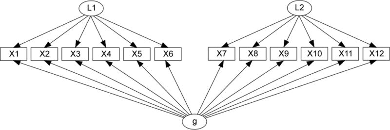
(a) Second–order model (b) Bi–factor model.

The part of the model that contains all of the variables but no edges between latent factors, is called the measurement model and the part of the model that contains only the latent factors and the edges between them is called the structural model.

In the simplest path diagram of a second–order measurement model, e.g., Figure 1(a), each indicator has one underlying “second-order” latent influence (the underlying latent construct g in Figure 1(a), which in turn has multiple primary factor sub-dimensions (the latent factors L₁ and L₂ in Figure 1(a)). Each indicator in a “pure” second-order model has only one latent sub-dimension for a parent, and all error terms are uncorrelated. In a “pure” bi–factor measurement model, each indicator has exactly two latent parents, one that is the general underlying factor (g in Figure 1(b), and one secondary group factor (L₁ and L₂ in Figure 1(b)), and again all error terms are uncorrelated.

Even if such models accurately approximate the causal structure underlying a set of measured indicators, there might also be additional but un–modeled complexity in the form of omitted latent common causes (factors), or indicators that are causally influenced by or have correlated errors with other indicators, or indicators that directly “load” onto more latent factors. For example, in Figure 2, the path diagram containing only black edges is a simple second–order model involving four latent factors L₁ – L₄, and one second–order factor g. Additional un–modeled complexity might arise from the green (correlated errors for X₁₃–X₁₇), blue (correlated errors for X₁₂–X₁₄), and red (an indicator that loads on more than one latent factor, e.g. X₂₀. We refer to measurement models that have no un–modeled complexity as “pure” measurement models.

Figure 2.

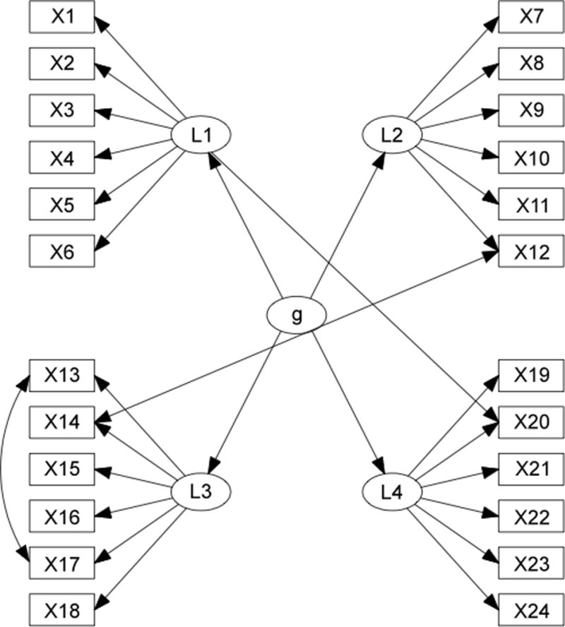
A second-order model with un-modeled complexities.

As we will show in the simulation study in Section 4, assuming 1) that the true generating model has a pure measurement model, and 2) that the true generating model is either a second–order or bi–factor model, then standard statistical measures can often correctly identify whether the data were generated by a second–order or bi–factor model (Morgan, Hodge, Wells, & Watkins 2015). If assumption 1 is false, but assumption 2 is true, then unsurprisingly, standard statistical measures applied to estimated pure bi–factor and second–order models do not typically correctly identify whether the data were generated by a second–order or bi–factor model. Indeed, Murray and Johnson point out that an estimated pure bi-factor model will typically fit data generated by an impure second-order model (that is, a model with extra un–modeled complexity) better that an estimated pure second-order model. If, however, before one knows whether the measurement model is bi–factor or second–order, one can locate a subset of indicators that are “pure” (that is, indicators that are not involved in any un–modeled complexity), then by using only the “pure” indicators one can use standard statistical measures on the bi-factor and second-order models to reliably determine whether the measurement model is in fact bi–factor or second–order.

For example, if, in Figure 2, one chooses any subset of the indicators that includes at most one of X₁₃ or X₁₇, at most one of X₁₄ or X₁₂, and does not include X₂₀ (for example the indicators in Figure 3) then the resulting subset of variables are in fact governed by a pure measurement model, and thus standard statistical measures can be used to identify the measurement model as second–order.

Figure 3.

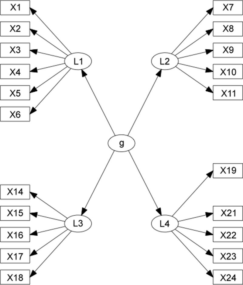
A sub-graph of Figure 2 that is “pure”.

Thus the strategy we will adopt in this paper is to search for a subset of the indicators that are pure, and then estimate bi-factor and second-order models involving only these variables.

First we introduce the terminology needed to more rigorously define a pure measurement model. A set of variables V is causally sufficient (has no unmeasured confounders) when every direct cause of any two variables in V is also in V. A set of variables V is minimally causally sufficient for O ⊆ V when V is causally sufficient, and no proper subset of V is causally sufficient and contains O.¹

In a second–order model, a subset of indicators that are effects of the same primary factor, and that have no correlated error with another indicator and are neither causes nor effects of any other variable, is a pure cluster. Similarly, in a bi–factor model, a subset of indicators that are effects of the same general and same group factor, and that have no correlated error with another indicator and are neither causes nor effects of any other variable is a pure cluster.

Any indicator that is the endpoint of an edge (directed or bi–directed) between two indicators is impure, as is any indicator that has more than one primary factor as a direct cause (in the case of second–order models) or more than one group factor as a direct cause (in the case of bi–factor models). The number of impure edges in a second-order model is calculated by adding one for each pair of indicators that has an edge (directed or bi–directed between them) and n−1 for each indicator that has n primary factors as direct causes. The number of impurities in a bi–factor model is calculated by adding one for each pair of indicators that has an edge (directed or bi–directed between them) and n−1 for each indicator that has n group factors as direct causes. Note that removing a single indicator can decrease the number of impure edges by more than one, since the indicator might be the endpoint of multiple edges between indicators or an endpoint of multiple edges from group factors.

In summary, we will show that by “purifying”, that is, by removing the impure indicators before comparing measurement models, one can often eliminate the bias of goodness-of-fit statistics described by Murray and Johnson that prefer bi–factor models even when the data generating process is second–order.

2. Comparing Second-Order and Bi-factor Models

Schmidt and Leiman(1957) showed that there is a transformation of any second–order model into a bi–factor model. Yung, Thissen and Mcleod (1999) showed that any second–order model transformed into a bi–factor model by a Schmid–Leiman transformation satisfies hidden proportionality constraints on the parameters of the bi–factor model, and these proportionality constraints encode extra rank constraints on the covariance matrix implied by a second–order model. In Appendix 1 we precisely characterize the constraints on the covariance matrix entailed by path diagrams. These constraints can be used to distinguish bi–factor models that are not compatible with any second–order model.

Conventional statistical measures used for structural equation model fit such as the BIC or chi-square have two components, a statistic measuring the deviance between the implied covariance matrix and the measured covariance matrix, and a correction for model complexity. The bi–factor model is more complex than the second–order model, and thus will be penalized more heavily in the BIC score and the chi–square test. For this reason, an estimated bi–factor model will have a smaller deviance than an estimated second–order model. Which model is preferred depends on the relative sizes of the deviances compared to the relative sizes of the complexity penalty. When data are generated from a pure bi–factor or pure second–order model, both the BIC and chi–square test tend to prefer the correct model. If the data are generated by a pure bi–factor model, the second–order model cannot typically achieve low enough deviance to be preferred, even though it is a simpler and thus carries a lower penalty for complexity than does the bi–factor model. If the data are generated by a pure second–order model, then the deviance for both models is typically low, but the bi–factor is penalized more heavily and thus the second-order model is preferred.

When the data are generated by an impure second–order model, but pure models are estimated and compared, then the bi–factor model tends to be preferred in proportion to the degree of impurity. The intuitive explanation for this phenomenon is that if the data are generated by a highly impure second–order model, then the deviance for a model specified and estimated as a pure second–order model will be quite high, but the deviance for a model specified and estimated as a pure bi–factor model will be much lower because the bi–factor model entails far fewer constraints and can thus be given parameter estimates that allow it to reasonably “fit” the data.

Haughton (1988) showed that in the large sample limit the BIC score would consistently choose a model M over any of its sub–models M ’ if the true distribution lay in M, but not in M ’, and that in the large sample limit the BIC score would consistently choose M ’ over M if the true distribution lay in M′. Niishi (1988) showed that under a set of regularity conditions, in the large sample limit both likelihood tests and BIC scores would consistently choose a model over a sub–model, when the true probability distribution lay in neither the model nor the sub–model.

If these theorems were directly applicable to the case of choosing between bi–factor and higher order models, then in the large sample limit, the BIC score would (i) consistently choose a pure second-order model (the sub–model) over a pure bi–factor model when the data was generated by a pure second-order model; (ii) would choose a bi–factor model over a second-order model when the data was generated by a bi–factor model that was incompatible with a second-order model;² (iii) choose a bi–factor model over a higher order model whenever the data was generated by an impure higher order or bi–factor model.

However, the observed marginal distributions of models with latent factors generally do not satisfy the regularity conditions that were assumed by Haughton(1988) or Niishi(1988), even if all of the variables are Gaussian. Whether their theorems can be extended to cases which satisfy the weaker set of conditions satisfied by the predicted marginal over the observed variables of Gaussian structural equation models with latent factors is not known, and hence neither Haughton’s nor Niishi’s results apply directly to the problem of distinguishing between bi–factor and second-order models. These theorems are suggestive, but do not settle the case. Hence, we will use simulations to examine the actual behavior of both likelihood tests and the BIC score in these various circumstances.

3. Algorithms

The algorithm that we describe for removing impurities depends on determining whether rank constraints on sub-matrices of the correlation matrix hold. Hence we will describe in more detail the rank constraints on sub–matrices of the covariance matrix that are imposed by the second–order model, but not the bi–factor model in the special case illustrated in Figure 1. A general rule for calculating the rank constraints entailed by a path diagram is presented in Appendix 1.

An n–tad constraint states that the rank of an n/2 by n/2 sub-matrix of the correlation matrix is n/2 − 1. For the 2 × 2 sub–matrix that contains the first row ρ(X₁,X₇), ρ(X₁,X₈) and the second row ρ(X₂,X₇), ρ(X₂,X₈) it is called a tetrad constraint and states that the rank of that 2 × 2 sub–matrix is equal to one, i.e. ρ(X₁,X₇), ρ(X₂,X₈) – ρ(X₁,X₈), ρ(X₂X₇) = 0. Similarly, for the 3 × 3 sub–matrix that contains the first row ρ(X₁,X₇), ρ(X₁,X₈), ρ(X₁,X₉), the second row ρ(X₂,X₇), ρ(X₂,X₈), ρ(X₂,X₉), and the third row, ρ(X₃,X₇), ρ(X₃,X₈), ρ(X₃,X₉) the constraint is called a sextad constraint and states that the rank of that 3 × 3 sub–matrix is equal to two.

The path diagram G of a structural equation model M is closely related to rank constraints on the covariance matrix. For example, the structure of the path diagram in Figure 1(a) entails that the tetrad constraint ρ(X₁,X₇) ρ(X₂,X₈) – ρ(X₁,X₈) ρ(X₂X₇) = 0 holds for all values of the error terms and all values of the linear coefficients. When a path diagram G entails that a rank constraint holds for all values of the free parameters of M, G entails the rank constraint.

In the models in Figure 1, ρ(X₁,X₇) ρ(X₂,X₈) – ρ(X₁,X₈) ρ(X₂X₇) = 0 is entailed by the path diagram in Figure 1(a) but not by the path diagram in Figure 1(b). Since second–order models are a proper subset of bi–factor models, it follows that there is some assignment of values to the free parameters of the bi–factor model in Figure 1(b) for which ρ(X₁,X₇) ρ(X₂,X₈) – ρ(X₁,X₈) ρ(X₂X₇) = 0.

In cases where there is some assignment of values to the free parameters for which a rank constraint holds, the rank constraint is compatible with the model. (A third possibility is that there may be no assignment of values to the free parameters of a model M for which a rank constraint holds, in which case the rank constraint is incompatible with M). For Bayesians, there is a sense in which a rank constraint that is compatible with, but not entailed by the path diagram of a model, is unlikely to occur for a very wide range, but not all priors over the linear coefficients. In all cases in which a rank constraint is compatible with, but not entailed by a model, for any continuous joint prior over the linear coefficients, the probability of a non-entailed rank constraint holding is zero. (See Spirtes et al. 2001). On the other hand, there are non-continuous priors in which it is not improbable that a rank constraint is compatible with, but not entailed by the path diagram of a model. For example, one way in which a bi–factor model can be compatible with a constraint that is not entailed by the path diagram of a bi–factor model is when all of the linear coefficients are equal. If there are particular facts about a domain that would lead a researcher to have a non-continuous joint prior over the linear coefficients but in which all of the linear coefficients have to be equal, the probability of a bi–factor model that is compatible with a constraint that is not entailed by its path diagram is not zero for that prior.

First we describe an algorithm for finding pure sub–models from data: Find One Factor Clusters or FOFC for short (Kummerfeld & Ramsey forthcoming, Kummerfeld et al. 2014). A more detailed description of this algorithm is given in Appendix 2. The FOFC algorithm is an algorithm for finding pure sub–models of a second–order (or correlated traits) model. It takes as input sample data, and outputs a partition of a subset of the original variables in which each cell contains a set of indicators that share the same latent primary factor in a pure second-order model. If FOFC is unable to find a pure second-order submodel, it outputs nothing. FOFC works by searching for a partition of a subset of the indicators that entails a set of tetrad constraints such that (a high percentage) of the tetrad constraints are judged to hold in the population by the delta test devised by Bollen and Ting (2000). Note that unlike clustering algorithms such as ICLUST (Revelle, 1978, 1979), or Detect (Zhang & Stout, 1999), FOFC does not require as input the number of clusters. FOFC is implemented in the TETRAD V software, that can be downloaded from (http://www.phil.cmu.edu/tetrad/current.html). An example of the use of the FOFC algorithm is available at www.phil.cmu.edu/tetrad/.

Given a covariance matrix for the variables X₁ through X₂₄, for example, if the true model is the second–order model shown in Figure 2, for a large enough sample size, the output of FOFC would be four clusters of variables {X₁, X₂, X₃, X₄, X₅, X₆}, {X₇, X₈, X₉, X₁₀, X₁₁}, {X₁₅, X₁₆, X₁₇, X₁₈}, and {X₁₉, X₂₁, X₂₂, X₂₃, X₂₄}. Each cluster is interpreted as having a single, distinct, latent factor, and together they form a pure second–order model. The indicators X₁₂, X₁₃, X₁₄, X₁₇, X₂₀ would not appear in any cluster in the output.³ In this paper, we will use the output of the FOFC algorithm in a slightly different way. We will remove all of the variables that are not included in the output from the FOFC algorithm (in this case, X₁₂, X₁₃, and X₂₀) but we will use background knowledge to cluster the remaining variables. This is a plausible use of the FOFC algorithm under the assumption that domain background knowledge is reliable for determining that a given set of indicator are all effects of a single primary factor, but that domain knowledge is unlikely to reliably indicate which indicators are impure.

One of the assumptions made by FOFC is that if a tetrad constraint is not entailed by the model’s causal structure (i.e., its path diagram), then the tetrad constraint does not hold in the population. This assumption is called “rank faithfulness” (Kummerfeld et al. 2014). Its justification is measure-theoretic. If a rank constraint is not entailed to hold for every possible parameterization of a path diagram G, but is compatible with G, then the set of values of the free parameters for which the rank constraint holds has zero probability for all continuous priors over the linear coefficients in G. Nevertheless, it is possible that there are many tetrad constraints that are not entailed by a path diagram, but that “almost” hold for many values of the free parameters. For example, “almost” violations of faithfulness can occur when the standardized edge coefficients are very close to one, or where the variance of the distribution of the edge coefficients is very small. Both of these cases can in principle be detected by estimating the edge coefficients of the bi–factor model. This still leaves the question of whether there are common “almost” violations of rank faithfulness that could only be discovered with enormous sample sizes (i.e. the relevant determinants are very close to zero), which we will address through simulation studies in section 4.

Since FOFC employs statistical tests to judge when tetrad constraints hold in the population, these “almost” holding tetrad constraints can mislead the algorithm on finite sample sizes. This is mitigated to some extent by the fact that the algorithm does not make incorrect outputs unless very particular sets of tetrad constraints are mistakenly judged to hold in the population.

We propose the following algorithm for deciding between a second–order model and a bi–factor model.

1. Run the FOFC algorithm, discard the variables that are not placed in any of the output clusters suggested by FOFC, and then re–cluster the remaining by using background knowledge.

2. If the output of FOFC has sufficiently many indicators that have not been removed from the model then

   1. Calculate the BIC score for the pure second–order model with the clusters from background knowledge but only involving the subset of variables output by FOFC.
   2. Calculate the BIC score for the pure bi–factor model with the clusters from background knowledge but only involving the subset of variables output by FOFC
   3. Accept the model with the lower BIC score.

3. Else reject the second–order model.

Clearly if FOFC outputs no pure indicators (i.e., it identifies all the indicators as impure), then the second–order model has in effect been rejected. Alternatively, the output might so drastically reduce the number of indicators that are detectibly pure that a researcher might choose to reject it anyway. Hence we leave it up to the researcher to decide the threshold for “sufficiently many indicators.” If the second–order model is rejected, the algorithm does not specify what to conclude about accepting or rejecting the bi–factor model. One possibility is to use the Find Two Factor Clusters algorithm (Kummerfeld et al. 2014) that is analogous to FOFC and can be applied to the same data to draw conclusions about accepting or rejecting the bi–factor model. However, we will leave a full discussion of that for another article.

4. Model Comparison Between Bi–factor Models and Second–order Models

The following simulation study shows how the FOFC algorithm works in practice. In this part of the project, we also investigate the way impurity, that is, un-modeled complexity, affects the model comparison results between bi–factor models and second–order models using various fit indices. The FOFC algorithm is used as an impurity removal procedure. We also investigate how impurity removal procedures help to recover the correct results of the above model comparison approach.

The population model is a second–order model with 4 clusters, each of which contains 6 indicators. We consider 3 types of impurities (un–modeled complexity) in the population model (see Figures 2 and 4): Correlated errors across group factors; Correlated errors within a group factor, and Cross-factor loadings. We choose this type of population model to illustrate the concepts. In a more systematic study, the number of clusters and the number of indicators in each cluster may be randomly generated from a reasonable range of values. Figure 4 shows the distribution of the values of the parameters in the data-generating SEM (where U(x,y) is the uniform distribution with lower limit x and upper limit y). These parameter values were chosen to produce correlation matrices that looked roughly realistic, i.e. they avoided both very small and very large correlations.

Figure 4.

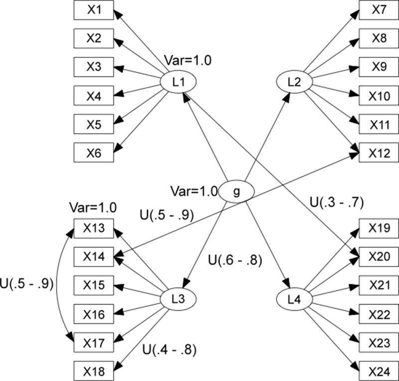
The distribution of the parameter values of the generating SEM.

For each graphical model, we generate 10 distinct instantiated models by randomly generating parameter values, and then generate 10 samples of size 500 for each of the instantiated models. The input to each algorithm is the sample covariance matrix. Because the quality of the output of FOFC varies depending upon features (including the variance) of the parameter values, we tested the algorithm over a wide variety of parameter values; hence, we used randomly generated parameter values rather than actual parameter values from a real model. However, we selected the parameter values from a range of parameter values we judged to occur in realistic models. We use each sample of data to estimate one pure bi–factor model and one pure second–order model with the same clustering as the population model, and compare several of their overall fit indices (RMSEA, BIC score and p-Value of the Chi-square test). We have chosen RMSEA, BIC, and the p-value of a Chi-squared test because they are commonly used, and theoretically justified. We did not observe significant difference in behavior between these three fit indices, so we did not investigate other fit indices. We used a conjugate direction minimization procedure for the F_ML score:

$$F_{\mathit{ML}}=\mathit{log}\left|\sum \left(\theta \right)\right|+tr\left(\mathit{S}{\sum }^{-1}\left(\theta \right)\right)-\mathit{log}\left|\mathit{S}\right|-\left(p\right),$$

where S is the sample covariance matrix, $\sum \left(\theta \right)$ is the implied covariance with parameter set θ, and p is the number of observed variables (in this case p=20). We then use FOFC as an impurity removal procedure to locate a set of impure indicators automatically.

The accuracy of the output of FOFC procedure is measured in two ways: e₁ (errors of omission) is the percentage of the number of impurities in the population model that are not uncovered by the procedure (i.e. false negatives); e₂ (errors of commission) is the percentage of the determined impure indicators that are actually pure in the population model (i.e. false positives). For example, if a population model contains {X₁ ↔ X₅, X₂ ↔ X₆, X₂ ↔ X₉}, and the removed indicators are {X₂, X₇, X₈}, then e₁ = 1/3, e₂ = 2/3.

We then remove the impure indicators from the data table, and estimate the two pure models using the resulting reduced variable data set and compare the fit indices again. The purpose is two-fold: (1) to show that the model comparison results are improved after the impurity removal procedure; and (2) to show that the accurate models (in this case the second–order model) have a better chance to pass a goodness-of-fit-test.

In the generating model, some indicators will be impure, others will be pure, and some impure indicators will be involved in many impurities. The distribution of impurities might matter a lot. In some cases, a small set of indicators might be involved in a lot of impurities and in others the un–modeled complexity might be evenly distributed among many of the indicators. For our procedure, having all the un–modeled complexity concentrated on a small set of indicators is favorable – as in that case removing a small number of indicators results in total purification as opposed to having to remove a large number of indicators before the sub-model is pure. One wants only a few bad apples.

We measure the unevenness of the distribution of any type of impurity as follows. The inhomogeneity of a distribution d of the impurities over the indicators is measured by a slight modification of the standard deviation SD of d described below. For example, when the number of impurities each indicator is involved in is exactly the same for all the indicators, the distribution d is perfectly homogeneous, SD_min = 0. On the other hand, if all of the impurities concentrate on 1 indicator, then d is maximally uneven and SD takes the largest value SD_max. Therefore we can define IH as the normalized standard deviation of the distribution of the number of impurities over all the indicators IH = (SD – SD_min)/(SD_max – SD_min), where SD_max and SD_min are the maximal and the minimal possible standard deviation of the distribution of the number of the impurities over all the indicators, given the pure DAG and the number of the five types of impurities. The value of IH ranges from 0 to 1, which correspond to the smallest and the largest possible standard deviation of the distribution respectively. From the parameter IH that the users specify, we can derive the corresponding standard deviation SD of the impurity distribution. There might not be any distribution with this standard deviation SD for the given pure DAG and the number of impurities, but we can aim at a distribution the standard deviation of which is closest to SD.

We found that the following 3 elements have significant effects on the results of model comparison: (i) the number of impurities; (ii) the degree to which the impurity influences the implied covariance matrix (parameterized by the edge coefficient assigned to the impurity); (iii) the degree of inhomogeneity. We describe the effects of each below.

First we consider the effect of the number of impurities on the ability of FOFC to detect impurities. In Figure 5 we show the percentage of impure indicators that are not detected as impure (false negatives). In this simulation, the omission error did not increase with the number of opportunities for omission. If anything the algorithm acts like the Spanish Inquisition – for any suspected impurity the indicator is removed.

Figure 5.

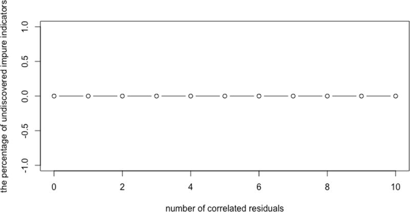
The percentage of impure indicators that are not detected as impure versus the number of correlated residuals.

In Figure 6 we show the percentage of pure indicators that are incorrectly classified as impure by the algorithm (false positives). In this case, the commission error starts very high (almost no indicator is actually impure but the algorithm is zealous), and as the number of impurities goes up its incorrect classifications go down.

Figure 6.

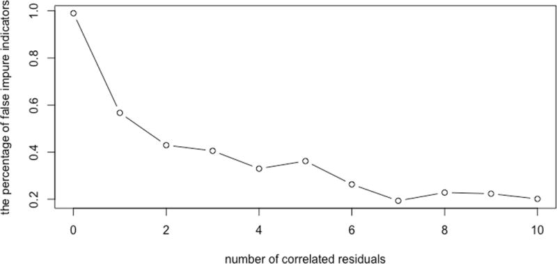
The percentage of pure indicators that are incorrectly classified as impure versus the number of correlated residuals.

Figures 7 and 8 illustrates how the number of impurities affect the model comparison results.

Figure 7.

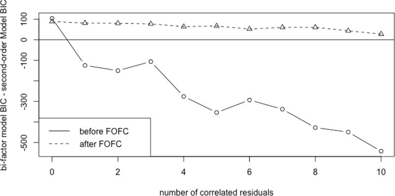
The difference in the estimated BIC scores between the bi-factor and second-order models versus the number of correlated residuals.

Figure 8.

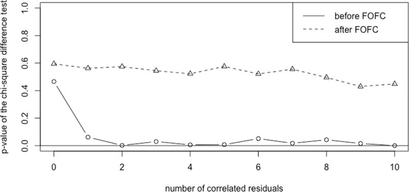
The p-values of the chi-square difference test between the bi-factor and second-order models before and after FOFC versus the number of correlated residuals.

The edge coefficient for each impure edge is drawn from a uniform distribution U(0.3, 0.4). The inhomogeneity level of the impurity distribution is set to 0.6. The alpha value for the delta test of vanishing tetrads used in the FOFC algorithm is 0.01.

In Figure 7 the horizontal axis represents the number of impurities within clusters added into the second–order population model. The vertical axis represents the BIC score of the estimated bi-factor model minus the BIC score of the estimated second-order model, averaged over the 10 × 10 repetitions of the simulation. Since the preferred model has a lower BIC score, when the difference in BIC scores (dBIC) between the second–order model and the bi–factor model is negative, the bi–factor model is preferred; when the difference in BIC score is zero, neither model is preferred; and when the difference in BIC scores is positive, the second–order model is preferred. Hence, a dBIC level above 0 indicates that the BIC comparison favors the second–order model, and a level below 0 indicates that the bi–factor model is preferred. The solid line (before FOFC purification) represents the case where the difference in BIC scores between a pure second–order model and a pure bi–factor model are calculated using all 24 indicators, where the clusterings are the ones given by the true second–order model. The dotted line (after FOFC) represents the case where the difference in BIC score between a pure second–order model and pure bi–factor model are calculated using only the subset of the 24 indicators that appear in the output of FOFC, where the clusterings are given by the true second–order model. If the true model is Figure 2, for example, and the output of FOFC left out the indicators X₁₂, X₁₃, X₁₄, and X₁₇ from the output, the BIC scores would be constructed from the pure second–order and pure bi–factor models with just those indicators removed.

The solid line (before FOFC) indicates that with no impurities, the second–order model is slightly preferred over the bi-factor, which is appropriate. At more than zero impurities, the dotted line indicates that the BIC score prefers the bi–factor model, and the preference becomes more pronounced as the number of impurities increases. This is exactly in accord with Murray and Johnson (2013) findings, where the amount of “un–modeled complexity” corresponds to the number of impurities.

In contrast, the behavior of the dotted line (after FOFC) is very different. With no impurities, the second–order model is again preferred. As the number of impurities increases, however, the BIC score still favors the second–order model, although the difference between the two models approaches zero as the number of impurities increases. This demonstrates that the FOFC algorithm has successfully found sub–models that are pure enough so that the BIC score correctly prefers the pure second–order model.

Figure 8 shows the p-value of the χ² difference test comparing the two pure models, both before and after the purification procedure. The solid line (before FOFC) indicates that the difference between the two nested models is significant when there is more than one impurity, which means that the more complicated bi-factor model is favored. The dotted line shows that after purification, the difference is not significant even if 20 impure edges are added to the original second-order model. This result shows that the application of FOFC significantly improves the accuracy of the χ² difference test to distinguish bi-factor models and second-order models.

Next, we describe how the strength of the impurities affects the results. Unsurprisingly, the results are also affected by the strength of the impurities, that is, the coefficient values of the edges or correlated errors that are the impurities. Again as a case study, consider 3 correlated residuals within clusters distributed over the indicators with a level of inhomogeneity of 0.4. Figure 9 shows how the preference of one model over another measured by estimated BIC score difference changes as the value assigned to the impurity edge coefficients increases. The pure second-order model is favored when the impurity parameters are smaller than approximately 0.3, but the bi–factor model if favored when the edge coefficient becomes larger.

Figure 9.

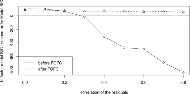
The difference in the estimated BIC scores between the bi-factor and second-order models before and after FOFC versus the parameter values of the impurities.

Finally, we describe how the degree of inhomogeneity affects the results. As a case study, consider 5 correlated residuals within clusters distributed over the indicators with distinct levels of inhomogeneity. The correlation of each of the un-modeled correlated residuals is set to 0.45. As the degree of inhomogeneity increases (which means that more of the impurity is concentrated on fewer indicators), the ability of the purification procedure in FOFC to find impurities goes up, and the number of pure indicators left behind increases as well. In Figure 10, we plot the degree of inhomogeneity against the dBIC. As predicted, the performance of the FOFC purification strategy improves as the level of inhomogeneity increases.

Figure 10.

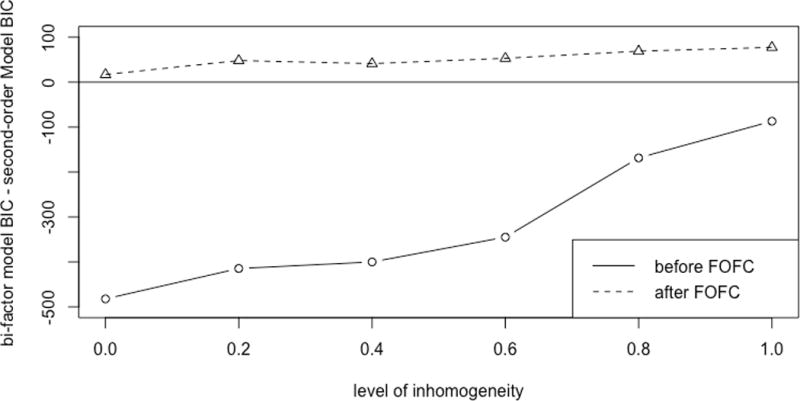
The difference in the estimated BIC scores between the bi-factor and second-order models versus the level of inhomogeneity.

5. Discussion

The second–order and bi–factor models are nested measurement models that are increasingly popular in contemporary substantive research in intelligence, personality and psychopathology. However, recent research has demonstrated that statistically differentiating these models is highly problematic if the second–order model is mis–specified as pure when the data generating model is second-order but also has un–modeled correlated residuals, cross–loadings on primary factors, and so on. In that case, standard fit measures are biased in favor of a bi–factor model even when the second–order is the true generating mechanism in the population (Murray & Johnson, 2013).

One possible method for choosing between a higher-order and a bi-factor model is to attempt to model the complexities that make the models impure, and then compare the impure higher-order model to the impure bi-factor model. One way of finding and modeling the impurities is through the use of modification indices, where one can start with an initial, given (in this case pure) model, and use modification indices to choose fixed parameters that should be freed (i.e. which edges should be added to the path model). There are a number of reasons to believe that modification indices would perform poorly in these circumstances, as simulation studies have shown (Spirtes et al., 1990). Modification indices suffer from problems of failure to converge, inaccuracy when the starting model is far from the true model, and getting stuck in local optima. For example, if, in the true model an indicator X₁ loads on latents L₁ and L₂, and causes another indicator X₁, then L₂ has an indirect effect on X₂ through X₁. If, in the specified model, however, X₁ only loads on latent L₁ and has no effect on X₂, then a modification index search will often free the parameter associated with the loading of L₂ on X₂, which is in fact 0 in the true model. Having made this “mistake” early in the modification index search, the additional parameters that search suggest to free are often far from the truth. However, a direct comparison between the use of modification indices and the algorithm proposed in this paper is something deserving of future research.

In this research, we propose one approach to addressing this model comparison problem. Specifically, we introduced an FOFC algorithm that “searches” the data in order to find pure indicator clusters. Model comparison tests are then conducted on this “purified” subset of indicators. To explore the viability of the proposed algorithm, we conducted a set of Monte Carlo simulations. The simulations indicated that the bias towards the bi–factor model over the second–order model increases as the number of impurities and the strength of the impurities increases, and the inhomogeneity of the impurities decreases. The FOFC reliably removed impure indicators even when the number of impurities as compared to the number of indicators was large, as long as the impurities were strong enough. The simulations also indicate that when the impure indicators are removed, that the bias towards the bi–factor model is removed, and the second–order model is preferred.

How useful FOFC would be in practice depends on a number of properties of real data. It may be that it is very rare that there are pure indicators for a wide variety of reasons, including correlated errors and mixtures of different causal structures in subpopulations. In psychometrics, there are often large numbers of indicators, so even if less than 50% are pure, there would still be enough pure indicators to form a pure sub-model. If pure indicators are even rarer, then using the FOFC algorithm is one way of discovering that, which would be an important fact about the limitations of current psychometric models. There is also a second algorithm, Find Two Factor Clusters (Kummerfeld et al. 2014), that uses a related set of rank constraints to look for “pure” bi-factor models, which can be employed in place of FOFC. Although these results are encouraging, further research into making the output of FOFC more reliable and more stable is needed, and empirical applications are also needed. As the ultimate goal of specifying a measurement model is often to find causal relations among the latent variables, more research is needed on how the measurement model specification influences our ability to estimate or detect relations among the latent variables (e.g., Bonifay, Reise, Scheines, and Meijer, 2015; Reise, Scheines, Widaman, and Haviland, 2013). Does mis–specifying a bi–factor model when the generating model is second–order (but impure) impact our ability to estimate the relationships between the latent modeled and other latents? Would purifying first help? To what degree?

Suppose for example, that the underlying purpose of a scientific investigation was to estimate the effect of extraversion on career success, controlling for self–esteem, where each of these variables is a latent construct to be measured with multiple indicators. If self–esteem was measured with a bi–factor model, but the true model was a second–order model with impurities, then what effect would mis–specifying the measurement model have on the estimate of the effect of extraversion on career success? Reise, Scheines, Widaman, and Haviland, 2013 showed that mis–specifying a measurement model for a latent L as unidimensional when it was in fact bi–factor had little effect on estimating the relations between L and other variables, so long as L explained a large proportion of the common variance among its indicators. Perhaps a similar result will hold in studies that mis–specify a model as bi–factor when it is in fact second–order with impurities.

Another interesting question to explore involves the trade–off between the number of indicators used and the amount of impurity in those indicators. If indicators are pure, then the more indicators in a model the better the estimates of the latent scores, the latent’s relationship with other latents, and so. Adding impure indicators to a measurement model will not have this effect, however. If an indicator is highly impure, then removing it will almost undoubtedly improve the statistical properties of the measurement model. If an indicator is mildly impure, however, the tradeoff might go either way. Research is needed on this trade–off.

Finally, we have assumed that the true measurement model is either bi–factor or second–order or correlated–error, but we don’t know how our procedure would perform if this assumption is false. We don’t know how assumptions of linearity and Gaussianity affect the validity of our procedures. Moreover, we don’t know how to handle situations in which different subjects in the sample are governed by different models, a situation we describe as a “mixture.” If some proportion of the subjects are filling out responses randomly, while the rest are acting in good faith, this presents a real problem for the task of distinguishing which measurement model best describes some population. In a sample of several hundred subjects, the difference between how a bi–factor and a second–order model fit the sample as judged by the BIC score or some derivative of the χ² test might be determined entirely by 15–20 subjects. If these subjects are acting randomly, and thus are “un–modelable,” then they might completely skew the parameters in use. Thus, another approach to distinguishing among measurement models might look to remove not only indicators that are detectably impure, but subjects that are “un–modelable.”

Appendix 1: Rank Constraints on Sub–Matrices of the Covariance Matrix

The rank constraints that hold are closely related to the structure of the path diagram of a model. In a given path diagram for either a pure second–order model or a pure bi–factor model, say that two variables occur in the same cluster if they have the same set of latent parents.

A simple trek in directed graph G from I to J is an ordered pair of directed paths (P₁; P₂) where P₁ has sink I, P₂ has sink J, and both P₁ and P₂ have the same source K, and the only common vertex among P₁ and P₂ is the common source K. One or both of P₁ and P₂ may consist of a single vertex, i.e., a path with no edges. There is a trek between a set of variables V₁ and a set of variables V₂ iff there is a trek between any member of V₁ and any member of V₂. Let A, B, be two disjoint subsets of vertices V in G, each with two vertices as members. Let S(A, B) denote the sets of all simple treks from a member of A to a member of B.

Let A, B, C_A, and C_B be four (not necessarily disjoint) subsets of the set V of vertices in path diagram G. The pair (C_A; C_B) t-separates A from B if for every trek (P₁; P₂) from a vertex in A to a vertex in B, either P₁ contains a vertex in C_A or P₂ contains a vertex in C_B; C_A and C_B are choke sets for A and B. Let #C be the number of vertices in C. For a choke set (C_A; C_B), #C_A + #C_B is the size of the choke set. We will say that a vertex X is in a choke set (C_A; C_B) if X ∈ C_A ∪ C_B.

For two sets of variables A and B, and a covariance matrix over a set of variables V containing A and B, let cov(A, B) be the sub-matrix of the covariance matrix that contains the rows in A and columns in B. The following two theorems relate the structure of the causal graph to the rank of sub-matrices of the covariance matrix.

Theorem 1. (Extended Trek Separation Theorem)

Suppose G is a path diagram without correlated errors or cycles containing C_A, A, C_B, and B, and (C_A; C_B) t-separates A and B in G. Then for all covariance matrices entailed by a linear structural equation model S with path diagram G, rank(cov(A, B)) ≤ #C_A + #C_B.

Theorem 2

For all path diagrams G without correlated errors or cycles, if there does not exist a pair of sets C, C′such that (C;C′) t-separates A and B and #C+ # C’≤ r, then for any C_A, C_B there is a linear structural equation model S with path diagram G for A and B that entails rank(cov(A, B)) > r .

Theorem 1 guarantees that trek separation entails the corresponding vanishing sextad for all values of the free parameters, and Theorem 2 guarantees that if the trek separation does not hold, it is not the case that the corresponding vanishing sextad will hold for all values of the free parameters.

Appendix 2: Algorithms

The FOFC algorithm searches for a clustering of variables that most closely implies the set of tetrad constraints judged by statistical tests to hold in the population. As illustrated in Figure 1, if S is a pure subset of indicators, every tetrad that contains three or more variables from S is entailed to be zero. In contrast, if S is an impure subset of indicators, there is a tetrad that contains three or more variables from S that is not entailed to be zero. So the algorithm searches for subsets S of indicators such that any tetrad containing three or more variables from S is judged to be zero by a statistical test. Impure indicators will not appear in any pure cluster, and will not be output in any cluster.

There are 3 × (n choose 4) possible tetrads for a given set of n indicators, and the worst case is that all of them have to be tested. These statistical tests dominate the computational complexity of the algorithm, and so the algorithm is O(n⁴). In practice it can easily be run on hundreds of indicators. Theorem 3 states that the only kind of impurities that FOFC cannot detect are impurities where one of the indicators has a common cause with the latent factor. This kind of impurity is not detectible by the algorithm, but is also not important, because it does not affect the estimate of the value of the latent parent from the indicators. Let L(X₁) denote the latent primary factor that is a parent of X₁.

Theorem 3

If a SEM S is a second–order linear model that has a pure measurement sub-model T, T has at least 4 indicators, and at least 3 indicators in each cluster, and the population distribution is “rank faithful” to the path diagram of the true second–order model, then the FOFC algorithm outputs a clustering in which any two variables in the same output cluster have the same primary factor parent. In addition, each output cluster contains no more than one impure indicators X₁ and X₂, which is on a trek whose source is a common cause of L(X₁) and X_1..

Bibliography

- Bartholomew DJ, Steele F, Moustaki I, Galbraith JI. The Analysis and Interpretation of Multivariate Data for Social Scientists. Chapman & Hall/CRC; 2002. (Texts in Statistical Science Series). [Google Scholar]
- Bollen K, Ting K. Confirmatory tetrad analysis. Sociological Methodology. 1993;23:147–75. [Google Scholar]
- Bollen KA. Structural Equations with Latent Variables. Wiley-Interscience; 1989. [Google Scholar]
- Bonifay W, Reise S, Scheines R, Meijer R. When are multidimensional data unidimensional enough for structural equation modeling? An evaluation of the DETECT multidimensional index. Structural Equation Modeling 2015 [Google Scholar]
- Canivez GL. Bifactor modeling in construct validation of multifactored tests: Implications for multidimensionality and test interpretation. In: Schweizer K, DiStefano C, editors. Principles and methods of test construction: Standards and recent advancements. Gottingen, Germany: Hogrefe; 2016. pp. 247–271. [Google Scholar]
- Gignac GE. The higher-order model imposes a proportionality constraint: That is why the bifactor model tends to fit better. Intelligence. 2016;55:57–68. [Google Scholar]
- Haughton DMA. On the Choice of a Model to Fit Data from an Exponential Family. The Annals of Statistics. 1988;16(1):342–355. [Google Scholar]
- Kummerfeld E, Ramsey J. Causal Clustering for 1-Factor Measurement Models. Knowledge Discovery in Databases. doi: 10.1145/2939672.2939838. (forthcoming) [DOI] [PMC free article] [PubMed] [Google Scholar]
- Kummerfeld E, Ramsey J, Yang R, Spirtes P, Scheines R. Causal clustering for 2-factor measurement models. In: Calders Toon, Esposito Floriana, Hüllermeier Eyke, Meo Rosa., editors. Machine Learning and Knowledge Discovery in Databases. 2014. pp. 34–49. (Volume 8725 of the series Lecture Notes in Computer Science). [Google Scholar]
- Molenaar D. On the distortion of model fit in comparing the bifactor model and the higher-order factor model. Intelligence. 2016;57:60–63. [Google Scholar]
- Morgan GB, Hodge KJ, Wells KE, Watkins MW. Are fit indices biased in favor of bi-factor models in cognitive ability research?: A comparison of fit in correlated factors, higher-order, and bi-factor models via Monte Carlo simulations. Journal of Intelligence. 2015;3(1):2–20. [Google Scholar]
- Nishii Ryuei. Maximum likelihood principle and model selection when the true model is unspecified. Journal of Multivariate Analysis. 1988;27(2):392–403. [Google Scholar]
- Reise S, Morizot J, Hays R. The role of the bi–factor model in resolving dimensionality issues in health outcomes measures. Quality of Life Research. 2007;16:19–31. doi: 10.1007/s11136-007-9183-7. [DOI] [PubMed] [Google Scholar]
- Reise S, Scheines R, Widaman K, Haviland M. Multidimensionality and Structural Coefficient Bias in Structural Equation Modeling: A Bifactor Perspective. Educational and Psychological Measurement. 2013;73(1) [Google Scholar]
- Revelle W. Hierarchical cluster analysis and the internal structure of tests. Multivariate Behavioral Research. 1979;14(1):57–74. doi: 10.1207/s15327906mbr1401_4. [DOI] [PubMed] [Google Scholar]
- Revelle W. ICLUST: A cluster analytic approach to exploratory and confirmatory scale construction. Behavior Research Methods. 1978;10(5):739–742. [Google Scholar]
- Rodriguez A, Reise SP, Haviland MG. Evaluating bifactor models: Calculating and interpreting statistical indices. Psychological methods. 2016;21(2):137. doi: 10.1037/met0000045. [DOI] [PubMed] [Google Scholar]
- Schmid J, Leiman JM. The development of hierarchical factor solutions. Psychometrika. 1957;22(1):53–61. [Google Scholar]
- Silva R, Glymour C, Scheines R, Spirtes P. Learning the structure of latent linear structure models. Journal of Machine Learning Research. 2006 Feb;7:191–246. [Google Scholar]
- Spirtes P, Glymour C, Scheines R. Causation, Prediction, and Search. Second. The MIT Press; 2000. (Adaptive Computation and Machine Learning). [Google Scholar]
- Spirtes P. Calculation of Entailed Rank Constraints in Partially Non-Linear and Cyclic Models. Proceedings of the Twenty-Ninth Conference Annual Conference on Uncertainty in Artificial Intelligence (UAI-13) 2013:606–615. [Google Scholar]
- Spirtes P, Scheines R, Glymour C. Simulation Studies of the Reliability of Computer-Aided Model Specification Using the TETRAD II, EQS and LISREL VI Programs. Sociological Methods & Research. 1990:3–66. [Google Scholar]
- Sullivant S, Talaska K, Draisma J. Trek Separation for Gaussian Graphical Models. Ann Stat. 2010;38(3):1665–1685. [Google Scholar]
- Zhang J, Stout W. The theoretical DETECT index of dimensionality and its application to approximate simple structure. Psychometrika. 1999;64(2):213–249. [Google Scholar]