An elaboration of theory about preventing outbreaks in homogeneous populations to include heterogeneity or preferential mixing

Abstract

The goal of many vaccination programs is to attain the population immunity above which pathogens introduced by infectious people (e.g., travelers from endemic areas) will not cause outbreaks. Using a simple meta-population model, we demonstrate that, if sub-populations either differ in characteristics affecting their basic reproduction numbers or if their members mix preferentially, weighted average sub-population immunities cannot be compared with the proportionally-mixing homogeneous population-immunity threshold, as public health practitioners are wont to do. Then we review the effect of heterogeneity in average per capita contact rates on the basic meta-population reproduction number. To the extent that population density affects contacts, for example, rates might differ in urban and rural sub-populations. Other differences among sub-populations in characteristics affecting their basic reproduction numbers would contribute similarly. In agreement with more recent results, we show that heterogeneous preferential mixing among sub-populations increases the basic meta-population reproduction number more than homogeneous preferential mixing does. Next we refine earlier results on the effects of heterogeneity in sub-population immunities and preferential mixing on the effective meta-population reproduction number. Finally, we propose the vector of partial derivatives of the reproduction number with respect to the sub-population immunities as a fundamentally new tool for targeting vaccination efforts.

1. Introduction

Human populations are heterogeneous, but all differences need not be modeled to answer any specific question. Immunity to vaccine-preventable diseases, for example, is heterogeneous within the United States (figures 1). Can differences among and within states be ignored in establishing vaccination coverage targets or monitoring progress in attaining them? The function used routinely for that purpose, the population-immunity threshold, involves the basic reproduction number, denoted ℜ₀. As this quantity is derived from a mathematical model, ascertaining its adequacy amounts to determining if the model from which it was derived is sufficiently detailed.

Figure 1.

Immunity to measles in the United States among a) children aged 19 to 35 months and b) adolescents aged 13 to 17 years for all 50 states and the District of Columbia from the 2012 National Immunization Surveys (http://www.cdc.gov/vaccines/imz-managers/coverage/nis/child/2012-released.html). Immunity was estimated as proportions of children with at least one and adolescents with two or more doses of MMR vaccine times efficacies of 92% and 95%, respectively. The curves are fitted beta distributions having shape parameters α = 208.39 and β = 40.65 for children and α = 83.98 and β = 12.52 for adolescents. Insofar as some adolescents have had one dose of MMR, figure 1b under-estimates their immunity to measles.

Mechanistic models are hypotheses about processes underlying natural phenomena. Simplicity is a virtue because it facilitates their evaluation. But the only way to ensure that one's model is not too simple is to compare results with those from models that include additional details that might affect them. In transmission modeling, one generally distinguishes sub-populations whose members have characteristics with which their risks of being infected or infecting others vary (e.g., age, gender, location). Levins (1) coined the term meta-population for any population whose members could be so stratified, although his own applications involved spatially-stratified populations.

Recently, Ball et al. (2) noted that the meta-population framework may preserve analytic tractability, unlike alternative means of incorporating salient structural heterogeneity, namely agent-based or network models. But they describe several challenges for modelers, among them clarifying the usefulness and limitations of systems of weakly coupled large sub-populations in modeling the spread of infections. Coupling strength determines a continuum whose limiting meta-populations behave as one or as multiple independent sub-populations. Here we endeavor to consolidate and extend the contributions of others who have considered intermediate situations.

Rates of person-to-person contact may vary with population density (e.g., be greater in urban than rural areas). They may also vary with personal characteristics (e.g., be greater among schoolchildren than younger and older people). The effect of such heterogeneity on ℜ₀, defined as the average number of secondary infections caused by a newly infectious person on introduction to a wholly susceptible population, was studied by Dietz (3), Anderson et al. (4), May and Anderson (5), and Diekmann et al. (6). These authors showed that, when mixing among sub-populations is proportional, ℜ₀ varies with the contact rate's variance and mean.

Nold (7) developed a more general mixing framework in which a fraction of one's contacts is reserved for members of one's own group and the complement is distributed proportionately among groups. Jacquez et al. (8) allowed this fraction to vary among groups. Barbour (9), Dye and Hasibeder (10), Hasibeder and Dye (11), and Adler (12) showed that ℜ₀ attains its maximum when individuals having high average per capita contact rates mix exclusively with each other.

May and Anderson (13, 14), Hethcote (15), and Hethcote and van Ark (16) considered heterogeneity in immunity. They concluded that the immunity above which newly introduced infectious persons would not cause outbreaks, to which we refer as the naïve population-immunity threshold, was greater in heterogeneous populations than apparent if homogeneity was incorrectly assumed. But Hethcote and van Ark argued that the difference was modest if transmission rates were not too dissimilar. None of these authors considered preferential mixing.

Recently, Fine et al. (17) reviewed the history and applications of the population-immunity threshold,¹ which was derived from a model of a proportionally-mixing homogeneous population. In the next section, we define a meta-population model and mixing function with which to evaluate the utility of this threshold when mixing is preferential or sub-populations are heterogeneous with respect to characteristics affecting their basic reproduction numbers.

2. Methods

We employ the simplest meta-population model capable of informing vaccination policy to illustrate the effects of heterogeneity in sub-population contact rates and immunities, together with preferential mixing, on the effective reproduction number. A glossary accompanies this section.

Our model comprises n sub-populations in which people are susceptible, S_i, infected and infectious, I_i, or removed, R_i (from the infection process by virtue of immunization or immunity following infection), μ is both the birth and death rate (introducing susceptible people without changing population size), p_i are proportions immunized at birth, λ_i are per capita forces (or hazard rates) of infection among susceptible people, and γ is the recovery rate. The rates μ and γ are the reciprocals of life expectancy and the mean infectious period, respectively.

$$\begin{array}{c}\frac{{\mathit{\text{dS}}}_i}{\mathit{\text{dt}}}=\mu N_i(1-p_i)-({\lambda }_i+\mu )S_i\\ \frac{{\mathit{\text{dI}}}_i}{\mathit{\text{dt}}}={\lambda }_i{S}_i-(\gamma +\mu )I_i,\\ \frac{{\mathit{\text{dR}}}_i}{\mathit{\text{dt}}}=\mu N_i{p}_i+\gamma I_i-\mu R_i,\\ N_i=S_i+I_i+R_i,i=1,\dots ,n\end{array}$$

The force of infection among susceptible members of sub-population i, ${\lambda }_i≔a_i\beta {\sum }_{j=1}^n{c}_{ij}(I_j/N_j)$, where β is the probability of infection upon contacting an infectious person, a_i is the average contact rate in sub-population i (activity henceforth), c_ij is the proportion of the i^th sub-population's contacts that are with members of the j^th sub-population, I_j/N_j is the probability that a proportionally encountered member of sub-population j is infectious, and n is the number of sub-populations.

We follow Jacquez et al. (8), who modeled contacts among sub-populations (mixing henceforth) as c_ij ≔ ε_iδ_ij + (1 − ε_i) f_j, where $f_j=(1-{\varepsilon }_j)a_j{N}_j/{\sum }_{k=1}^n(1-{\epsilon }_k)a_k{N}_k$, ε_i is the fraction of their contacts that members of the i^th sub-population reserve for others in sub-population i (preference henceforth), and δ_ij is the Kronecker delta, taking value 1 when i = j and 0 otherwise. Thus, the complement of ε_i is distributed among all sub-populations including i in proportion to f_j, which describes activity-weighted proportional mixing. Jacquez et al. used this model for groups differing in sexual activity, but sub-population members could differ in age, location (e.g., reside in different households, in a city or surrounding villages), gender, or other discrete characteristics.

We limit n = 2 for transparency (i.e., analytical solutions are unwieldy, if possible to obtain, and graphing meta-population reproduction numbers or functions thereof against sub-population immunities, as we do in figures 2-8, is difficult when n > 2), but such calculations may be performed for any n. Indeed, the motivating application for this review and refinement of theoretical results is an assessment of vaccination among children attending elementary schools,² where n = 200 in the largest school district and n = 638 in the entire county. In such applications, effects that are modest when n = 2 become substantial.

Figure 2.

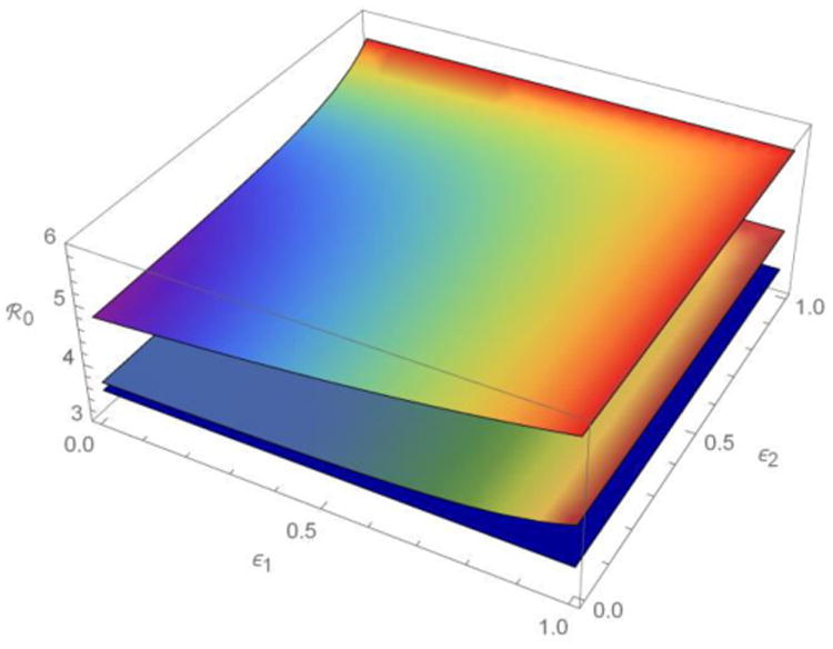
The meta-population ℜ₀ as a function of fractions of the contacts that members of two sub-populations reserve for others within their own sub-populations (ε₁, ε₂) when their activities (average contact rates) are more or less heterogeneous. ℜ₀ decreases from the top surface (a₁ = 4, a₂ = 16), through the middle (a₁ = 8, a₂ = 12), to the bottom (a₁ = a₂ = 10). See table 1 for other parameter values. As heterogeneity in ε(e.g., ratio of the variance and mean) increases away from the line ε₁ = ε₂, heterogeneous preferential mixing also increases ℜ₀.

Figure 8.

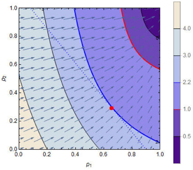
A numerical solution to the Lagrange problem. We observe that the line p₂ = (c − p₁N₁)/N₂ (dotted) is tangent only to the contour curve ℜ_v(p₁, p₂) = 2.2. They intersect at the point (p₁, p₂) = (0.66, 0.29), the optimal solution (marked with a red dot). The parameter c = 0.9 × N₁ with others the same as in figure 7. For some parameter values, the optimal solution might be outside the unit square in the p₁-p₂ plane.

For ease of reference, we define several terms based on the properties of (ε₁, ε₂, …, ε_n):

1. Mixing is proportional if ε_i = 0 for all i (i.e., contacts are proportional to f, a function described above).

2. Mixing is preferential if 0 < ε_i ≤ 1 for some i (i.e., a fraction ε_i of the contacts of members of sub-population i are with others in their own sub-population and its complement is distributed proportionally among all sub-populations).

3. The i^th sub-population is isolated (i.e., members mix only with others in their own sub-population) if ε_i = 1.

4. The preferential mixing is homogeneous if ε_i = ε for all i.

5. The preferential mixing is heterogeneous if ε_i ≠ ε_j for some i ≠ j.

3. Results

First we derive the reproduction numbers for our model meta-population, whose sub-populations may differ in subscripted variables (numbers susceptible, infectious and recovered; proportions vaccinated at birth; contact rates and fractions within and among groups). Consequently, our model is more general than that of Goldstein et al. (18), whose households are populated by different numbers of identical individuals. Then we explore the impact of heterogeneity in activity, a_i, and immunity, p_i, on these numbers. Finally, we explore the interplay between such heterogeneity and preferential mixing (some ε_i ≠ 0).

3.1 Reproduction Numbers

In our model, the basic and effective reproduction numbers for sub-population i, denoted ℜ_0i and ℜ_vi, respectively, which differ by vaccination as denoted by subscript v, are

$${\mathrm{R}}_{0i}=\frac{\beta a_i}{\gamma +\mu },{\mathrm{R}}_{\mathit{\text{vi}}}={\mathrm{R}}_{0i}(1-p_i).$$

Meta-population reproduction numbers are properties of next-generation matrices (19, 20) that translate vectors composed of the numbers infectious in each sub-population at one time (e.g., outbreak generation) into the corresponding vectors at other times (or generations). The largest eigenvalue is the average factor by which successive vectors differ in magnitude, or average number of secondary infections per infectious person, at equilibrium.

We derive the next-generation matrix K for the simplest meta-population (with n = 2) in appendix 1 (and, to dispel the notion that this somehow limits the generality of our arguments, n = 3 in appendix 2). When n = 2, $K=\left[\begin{array}{cc}{\mathrm{R}}_{v1}{c}_{11}& {\mathrm{R}}_{v1}{c}_{12}\\ {\mathrm{R}}_{v2}{c}_{21}& {\mathrm{R}}_{v2}{c}_{22}\end{array}\right]$, whose larger eigenvalue,

$${\mathrm{R}}_v=\frac{1}{2}[A+D+\sqrt{{(A-D)}^2+4BC}],$$

where A = R_v1c₁₁, B = R_v1c₁₂, C = R_v2c₂₁, D = R_v2c₂₂. If 0 < ε⃑ < 1, one cannot generally write explicit expressions for the meta-population ℜ_v when n > 4, but can always compute it numerically. The contributions of sub-population characteristics and preferential mixing that are described in the following sections depend on the structure of the next-generation matrix K, which could be written as the product of a diagonal matrix whose elements are ℜ_vi and matrix whose elements are c_ij.

3.2 Population Heterogeneity

As shown originally by Dietz (3), and subsequently by Anderson et al. (4), May and Anderson (5), and Diekmann et al. (6), when mixing is proportional, the basic reproduction number can also be written as

$${\Re }_0={\overline{\Re }}_0+\frac{\beta }{\gamma +\mu }\times \frac{{\sigma }^2}{m},$$

where ℜ̄₀ is the mean ℜ₀, and m and σ² are the mean and variance of activity among sub-populations. We observe that similar expressions could be derived for any characteristic affecting ℜ_0i. The probability of infection on contact with an infectious person might reflect age-specific differences in susceptibility, β_i, for one example, or the recovery rate reflect location-specific differences in medical care, γ_i, for another.

We find the spectral radius (eigenvalue of greatest magnitude) of the matrix K more intuitive because it generalizes easily to preferential mixing. But we derive this classic result mostly to demonstrate that such heterogeneity increases ℜ₀ even when mixing is proportional, and also because some of its many variations are incorrect. We also provide an example where two meta-populations have the same mean activity, but differ in their variances. In table 1, heterogeneity in sub-population activities increases ℜ₀ from 3.50 to 3.72 for proportional mixing (ε₁ = ε₂ = 0) and preferential mixing (ε₁ = ε₂ = 0.5) further increases it to 3.88. Evidently preferential mixing magnifies the effect of heterogeneity in activity, one sub-population characteristic affecting ℜ_0i in our simple meta-population model.

Table 1.

Preferential Mixing Magnifies the Impact of Heterogeneity in Person-to-Person Contact Rates (activity) on ℜ₀. The number of sub-populations and their sizes also affect these results, but here n = 2, N₁ = 500 and N₂ = 500, so that the mean activity is the same in scenarios A and B. Common parameters: β = 0.05, γ = 1/7, and N₁ = N₂ = 500 unless otherwise specified in figure or table legends.

	Scenario A		Scenario B
Parameter	a1 = 10	a2 = 10	a1 = 7.5	a2 = 12.5
ℜ0i	3.5	3.5	2.62	4.37
ℜ0 (ε1 = ε2 = 0)	3.5		3.72
ℜ0 (ε1 = ε2 = 0.5)	3.5		3.88
ℜ0 (ε1 = 0.25, ε2 = 0.75)	3.5		3.92
ℜ0 (ε1 = 0.75, ε2 = 0.25)	3.5		3.98

Figure 2 complements the empirical analyses tabulated, showing how heterogeneity in preference, another sub-population characteristic affecting ℜ_0i, modifies the effect of heterogeneity in activity. Consider the case when n = 2 with fixed total activity a_T ≔ a₁ + a₂, and all other parameters identical for the two sub-populations except ε_i. In appendix 3, we show that:

1. for ε₁ = ε₂ = 0, ℜ₀(0, 0) is minimized when a₁ = a₂ = a_T/2 and is a monotonically increasing function of the difference |a₂ − a₁| (i.e., ℜ₀ is maximized when heterogeneity in activity is greatest);

2. a similar result as in (i) holds when either ε₁ = 1 or ε₂ = 1. That is, ℜ₀(ε₁, 1) = ℜ₀(1, ε₂) as shown in appendix 3. This is minimized when a₁ = a₂ = a_T/2 and is a monotonically increasing function of the difference |a₂ − a₁|. Therefore, ℜ₀(ε₁, 1) = ℜ₀(1, ε₂) is maximized when heterogeneity in activity is greatest.

3.3 Mixing among Sub-Populations

Preference, the fraction of contacts reserved for one's own sub-population, ranges over the unit interval, but we can derive explicit limiting conditions (i.e., ε⃑ = 0, ε⃑ = 1) from our equations for the meta-population reproduction numbers when n = 2.

Case 1 (isolated sub-populations): When ε₁ = ε₂ = 1, we have c₁₁ = 1, c₁₂ = 0, c₂₁ = 0, c₂₂ = 1. Thus, in the expression above for the largest eigenvalue of the next-generation matrix K,

$$\begin{array}{c}A={\mathrm{R}}_{v1},B=0,C=0,D={\mathrm{R}}_{v2},\text{and}\\ {\mathrm{R}}_v=\frac{1}{2}[{\mathrm{R}}_{v1}+{\mathrm{R}}_{v2}+\sqrt{{({\mathrm{R}}_{v1}-{\mathrm{R}}_{v2})}^2}]=\{\begin{array}{cc}\frac{1}{2}[{\mathrm{R}}_{v1}+{\mathrm{R}}_{v2}+{\mathrm{R}}_{v1}-{\mathrm{R}}_{v2}]={\mathrm{R}}_{v1},& \text{if}{\mathrm{R}}_{v1}>{\mathrm{R}}_{v2}\\ \frac{1}{2}[{\mathrm{R}}_{v1}+{\mathrm{R}}_{v2}+{\mathrm{R}}_{v2}-{\mathrm{R}}_{v1}]={\mathrm{R}}_{v2},& \text{if}{\mathrm{R}}_{v1}<{\mathrm{R}}_{v2}\end{array}.\end{array}$$

That is, R_v = max{R_v1, R_v2}. When p₁ = p₂ = 0, we have ℜ_vi = ℜ_0i, whereupon R₀= max{R₀₁, R₀₂}.

Case 2 (proportionally mixing sub-populations): When ε₁ = ε₂ = 0, we have c₁₁ = f₁, c₁₂ = f₂, c₂₁ = f₁, c₂₂ = f₂. Thus, A = R_v1 f₁, B = R_v1f₂, C = R_v2f₁, D = R_v2f₂, and

$${\mathrm{R}}_v=\frac{1}{2}[{\mathrm{R}}_{v1}{f}_1+{\mathrm{R}}_{v2}{f}_2+\sqrt{{({\mathrm{R}}_{v1}{f}_1-{\mathrm{R}}_{v2}{f}_2)}^2+4{\mathrm{R}}_{v1}{f}_2{\mathrm{R}}_{v2}{f}_1}]=\frac{1}{2}[{\mathrm{R}}_{v1}{f}_1+{\mathrm{R}}_{v2}{f}_2+\sqrt{{({\mathrm{R}}_{v1}{f}_1+{\mathrm{R}}_{v2}{f}_2)}^2}]={\mathrm{R}}_{v1}{f}_1+{\mathrm{R}}_{v2}{f}_2.$$

When p₁ = p₂ = 0, we have ℜ_vi = ℜ_0i, whereupon R₀ = R₀₁f₁ + R₀₂f₂. Chow et al. (21, Section 3.1) proved that ∂ℜ_v/∂ε_i > 0 (i = 1, 2) for all 0 ≤ ε_i < 1, affirming earlier conjectures (8-11).

Goldstein et al. (18) define several reproduction numbers, among them the average number of infections in other households caused by an infected member of an index household. If we consider our meta-population ℜ_v = ℜ_v(ε₁, ε₂) as a function of ε₁ and ε₂, we can solve for the critical value of ε_1c at which ℜ_v(ε_1c, ε₂) = 1 for any given value of ε₂. Recall that

$${\mathrm{R}}_v=\frac{1}{2}[A+D+\sqrt{{(A-D)}^2+4BC}],$$

where A(ε₁, ε₂) = R_v1c₁₁, B(ε₁,ε₂) = R_v1c₁₂, C(ε₁,ε₂) = R_v2c₂₁, D(ε₁,ε₂) = R_v2c₂₂ with

$$\begin{array}{c}{c}_{11}={\epsilon }_1+\frac{{(1-{\epsilon }_1)}^2{a}_1{N}_1}{(1-{\epsilon }_1)a_1{N}_1+(1-{\epsilon }_2)a_2{N}_2},c_{12}=\frac{(1-{\epsilon }_1)(1-{\epsilon }_2)a_2{N}_2}{(1-{\epsilon }_1)a_1{N}_1+(1-{\epsilon }_2)a_2{N}_2},\\ c_{21}=\frac{(1-{\epsilon }_1)(1-{\epsilon }_2)a_1{N}_1}{(1-{\epsilon }_1)a_1{N}_1+(1-{\epsilon }_2)a_2{N}_2},c_{22}={\epsilon }_2+\frac{{(1-{\epsilon }_2)}^2{a}_2{N}_2}{(1-{\epsilon }_1)a_1{N}_1+(1-{\epsilon }_2)a_2{N}_2}.\end{array}$$

Note that ℜ_v(ε₁, ε₂) is an increasing function of ε₁ (21). Hence, if ℜ_v(0, ε₂) > 1, then ℜ_v(ε₁, ε₂) > 1 for all ε₁. If ℜ_v(0, ε₂) < 1, however, we can solve the equation ℜ_v(ε₁, ε₂) = 1 for ε₁ and arrive at

$${\epsilon }_{1c}=\frac{a_1{N}_1({\mathrm{R}}_{v1}-1)(1-{\mathrm{R}}_{v2}{\epsilon }_2)+a_2{N}_2({\mathrm{R}}_{v2}-1)(1-{\epsilon }_2)}{a_1{N}_1({\mathrm{R}}_{v1}-1)(1-{\mathrm{R}}_{v2}{\epsilon }_2)+a_2{N}_2{\mathrm{R}}_{v1}({\mathrm{R}}_{v2}-1)(1-{\epsilon }_2)}.$$

This expression provides a formula for ε_1c that is feasible if and only if the other parameter values are such that 0 < ε_1c < 1. Thus, ε_1c provides a critical value for ℜ_v = 1. This formula holds if ℜ_v is replaced by ℜ₀ (with ℜ_vi being replaced by ℜ_0i) as long as ℜ₀(0, ε₂) < 1.

3.4 Heterogeneous Preferential Mixing

Colizza and Vespignani (22) note that heterogeneity in connectivity, by which they represent individual movement in a spatial meta-population, increases the reproduction number. While our meta-population need not be spatial, distributing the 1 − ε_i contacts not reserved for members of sub-population i generally requires movement. Returning to table 1, we see that while preferential mixing (ε_i = ε₂ = 0.5) among sub-populations differing in ℜ_0i increases the meta-population ℜ₀ compared to proportional mixing (ε_i = ε₂ = 0), heterogeneous preferential mixing (ε_i = 0.25, ε₂ = 0.75 or vice versa) increases ℜ₀ compared to homogeneous preferential mixing (from 3.88 to 3.92 or 3.98). When n = 2, if either sub-population is isolated (ε₁ = 0, ε₂ = 1 or vice versa), both are isolated (appendix 3), whereupon ℜ₀ = max{ℜ₀₁, ℜ₀₂} = 4.37 as noted in the previous section. Apolloni et al. (23) consider social as well as spatial strata, neither however differing in as many respects as sub-populations in our single stratification. Comparable results are similar, affirming our conclusion that differences among sub-populations in factors affecting their reproduction numbers matter, not the means by which such heterogeneity arises.

3.5 Heterogeneity in Immunity

Figures 3 illustrate the impact of heterogeneity in p_i on ℜ_v in meta-populations whose sub-populations are the same size (scenario B of table 1), but mix proportionally and preferentially on the left and right, respectively. Heterogeneity increases away from the line of equality connecting the points at which (p₁, p₂) = 0 and (p₁, p₂) = 1. Values of ℜ_v for all combinations of p_i (i = 1, 2) form a plane when mixing is proportional, but curve upward about the above-mentioned line when mixing is preferential. Values at or below their intersection with the dark blue plane, ℜ_v = 1, are combinations of p_i (i = 1, 2) at which population-immunity attains or exceeds this threshold.

Figure 3.

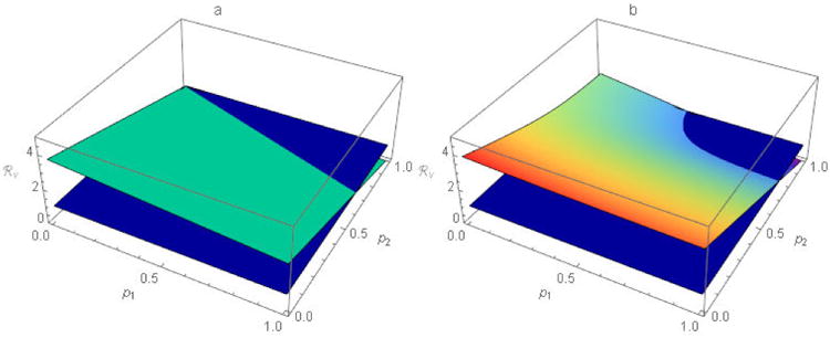
The function ℜ_v for scenario B of table 1 with a) proportional, and b) preferential, mixing. The dark blue planes represent ℜ_v = 1 and the lighter blue plane and curved (rainbow) surface represent ℜ_v for other tabulated parameters at all possible (p₁, p₂) pairs when a) ε₁ = ε₂ = 0 and b) ε₁ = ε₂ = 0.5, respectively. ℜ_v ≤ 1 for all combinations of p_i (i=1, 2) at or below the dark blue plane. While there is no single population-immunity threshold when n > 1, ℜ_v retains its utility as a threshold for outbreak prevention and, ultimately, disease elimination.

Because mixing affects ℜ_v, the impact of heterogeneity in p cannot be assessed absent information about mixing. Setting ε₁ = ε₂ = ε, for example, we observe that for fixed 0 < ε < 1 a curve in the p₁-p₂ plane divides the region 0 ≤ p₁ ≤ 1, 0 ≤ p₂ ≤ 1 into sub-regions such that ℜ_v > 1 (< 1) for (p₁, p₂) below (above) the curve (figures 4). Moreover, the area below (above) the curve increases (decreases) as ε increases. This suggests that the more preferentially sub-populations mix (higher ε⃑), the more difficult outbreak prevention becomes (i.e., the greater the requisite values of p⃑).

Figure 4.

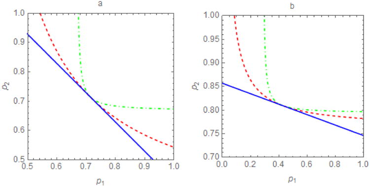
Contour plots of the threshold ℜ_v = 1 in the p₁-p₂ plane for different per capita contact rates, a, and proportions within-group, ε. For proportional mixing (ε⃑ = 0), the threshold pairs (p₁, p₂) for outbreak prevention or control form a (dark blue) line, p₂ = −bp₁ + r, where r > 0 is a constant and b=1 when a) sub-populations are identical in characteristics affecting ℜ₀ (here a₁ = a₂ = 10) and b) b≠1 when they differ (here a₁ = 5, a₂ = 15). At the other extreme, isolated sub-populations (ε⃑ = 1), the region in which ℜ_v < 1 is a rectangle. In between, dashed curves represent selected 0 < ε⃑ < 1 (red, ε₁ = ε₂ = 0.5; green, ε₁ = ε₂ = 0.75). These thresholds divide the plane into sub-regions such that ℜv >1 (ℜ_v < 1) below (above) the line or curve. Preferential mixing increases the difficulty of achieving ℜ_v =1. When ε= 1, pairs (p₁, p₂) must be within a relatively small rectangular area in the upper right quadrant. When ε = 0, pairs (p₁, p₂) need only be in the larger area above the solid line.

When ε = 0 and ε = 1, the regions in which ℜ_v > 1 and ℜ_v < 1 are a (possibly truncated) triangle and rectangle, respectively. The shapes of these regions depend on whether sub-populations are isolated (ε = 1), in which case the threshold immunities are independent (and thus horizontal or vertical lines), or their members mix proportionally (ε = 0), in which case the meta-population threshold depends on the immunity levels of both sub-populations (and thus a line that is neither horizontal nor vertical). The slope of this line depends on the values of parameters affecting ℜ_0i, the average contact rate or activity (a₁ and a₂) in our meta-population model. Vaccinating the sub-population whose members have higher per capita contact rates would more effectively reduce ℜ_v.

There is one exception. The curves intersect the straight line in figures 4 at the point (1 − 1/ℜ₀₁, 1 − 1/ℜ₀₂), at which ℜ_v1 = ℜ_v2 = 1, whereupon the next-generation matrix

$$K_v=\left[\begin{array}{cc}{\Re }_{v1}& 0\\ 0& {\Re }_{v2}\end{array}\right]\left[\begin{array}{cc}{c}_{11}& c_{12}\\ c_{21}& c_{22}\end{array}\right]=\left[\begin{array}{cc}{c}_{11}& c_{12}\\ c_{21}& c_{22}\end{array}\right],$$

whose dominant eigenvalue is 1∀ε.

Using a model meta-population composed of a city and several villages, May and Anderson (13, 14) showed that heterogeneity in relevant sub-population characteristics also increased ℜ_v. Hethcote and van Ark (16) argued that person-to-person contact rates in densely-populated urban areas should be no more than twice those in sparsely-populated rural ones. This change in parameter values diminished the apparent effect of heterogeneity. Our more transparent example (table 2) demonstrates that the effect on ℜ₀ (and, as ℜ_v is a function of ℜ₀, on ℜ_v as well) is greater when mixing is preferential (ε₁ = ε₂ ≠ 0) than proportional (ε₁ = ε₂ = 0) if sub-population sizes are equal (e.g., both 0.5N). When 90% of the people are in one sub-population and 10% in another (e.g., a city and village), our results resemble Hethcote's and van Ark's.

Table 2.

Sub-Population Sizes Affect the Impact of Heterogeneity in Activity and Preferential Mixing on ℜ₀. When sub-population sizes are unequal, as in scenario C, the larger dominates, but when they are equal, as in scenario D, heterogeneity and preferential mixing have greater impact. Other parameters: N = 1000, a₁ = 5 and a₂ = 10 (the village and city if N₁ ≪ N₂).

	Scenario C		Scenario D
Parameter	N1 = 0.1N	N2 = 0.9N	N1 = 0.5N	N2 = 0.5N
ℜ0i	1.75	3.5	1.75	3.5
ℜ0 (ε1 = ε2 = 0)	3.41		2.92
ℜ0 (ε1 = ε2 = 0.5)	3.44		3.09
ℜ0 (ε1 = 0.25, ε2 = 0.75)	3.42		3.12
ℜ0 (ε1 = 0.75, ε2 = 0.25)	3.46		3.2

In figures 5, we refine May's and Anderson's (13) conclusion that “under a uniformly applied immunization programme, the overall fraction that must be immunized is larger than would be estimated by (incorrectly) assuming the population to be homogeneously mixed.” Preferential mixing curves the level contours of ℜ_v in the p₁-p₂ plane that otherwise would be straight lines. Consequently, uniform immunization (p₁ = p₂) of meta-populations composed of sub-populations that are identical in characteristics affecting ℜ_0i does indeed attain ℜ_v =1 (or any other value) most efficiently. When sub-populations differ in such characteristics, however, this is no longer true (e.g., Keeling's and Rohani's (24) figure 3.3 resembles our figure 5b). In general, the optimal strategy vaccinates members of the sub-population whose ℜ_0i is greatest disproportionately.

Figure 5.

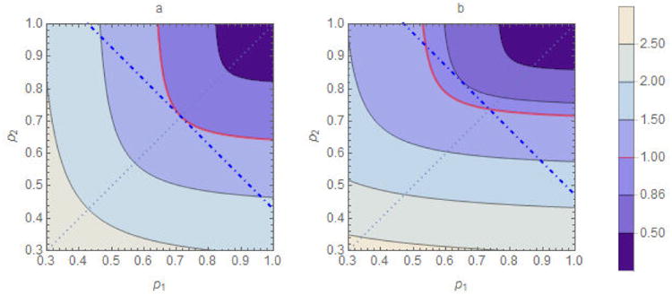
Comparison of homogeneous (p₁ = p₂) and heterogeneous immunity (p₁ ≠ p₂) when mixing is preferential (0 < ε₁, ε₂ ≤ 1). The parameter values are β = 0.05, γ= 1/7, ε₁ = ε₂ = 0.6, and N₁ = N₂ = 500. In figure a), a₁ = a₂ = 10, in which case ℜ₀ = 3.5. The solid curves are contours of the function ℜ_v(p₁, p₂) with the thicker (red) curve corresponding to ℜ_v = 1. The lighter (dotted) p₂ = p₁ line indicates homogeneous coverage; its intersections with the contour curves represent corresponding ℜ_v values. The homogeneous coverage required to achieve ℜ_v = 1 is p₁ = p₂ = 1−1/ℜ₀ = 0.71. The thicker dot-dashed line passing through point (p₁, p₂) = (0.71, 0.71) identifies all (p₁, p₂) pairs requiring the same number of vaccine doses in sub-populations of the same size (i.e., they satisfy p₁ + p₂ = 2×0.71). Its intersections with the contour curves also represent corresponding ℜ_v values. Note that ℜ_v > 1 for all (p₁, p₂) pairs other than (0.71, 0.71). In figure b), where a₁ = 8, a₂ = 12, in which case ℜ₀ = 3.8. The homogeneous coverage required to achieve ℜ_v = 1 is p₁ = p₂ = 1−1/ℜ₀ = 0.74. We observe some pairs with p₁ < 0.74 for which ℜ_v < 1, for one of which ℜ_v = 0.86.

Fine et al. (17) provide an example with n = 2 in which ℜ₀₁ = 5 and ℜ₀₂ = 1 and ℜ₀ = 5, so their sub-populations must be isolated (i.e., ε₁ = ε₂ = 1, whereupon c₁₂ = c₂₁ = 0). They state, “Because the high-risk group is responsible for any increase in incidence, outbreaks could in theory be prevented by vaccinating 80% of the high-risk group alone, thus, < 80% of the entire population.” This is true, but only because their meta-population is composed of isolated sub-populations. Keeling and Rohani (24) state that “In structured models, the critical level of vaccination that eradicates infection is the same as in unstructured models, 1 − 1/ℜ₀, if vaccination is applied at random,” which is true only if ℜ₀ is correctly specified. And ℜ₀ in structured and unstructured populations differ. Assuming, in the example of Fine et al., that β = 0.05, γ = 0.15, μ = 0 and that sub-population sizes are the same, we have a₁ = 15 and a₂ = 3. Averaging these contact rates, which is tantamount to assuming a proportionally-mixing homogeneous population, ā = 9, whereupon ℜ₀ = 3 and the naïve population-immunity threshold, p_c = 0.67. Contact heterogeneity (a₁ = 15 and a₂ = 3) increases ℜ₀ to 4.3, while preferential mixing (ε₁ = ε₂ = 1) further increases it to 5.

3.6 The Negative Gradient

Evidently ℜ_v depends not only on the immunity, p_i of sub-populations i, but also on the fractions of contacts, ε_i that members reserve for others in their own sub-populations, and their proportional mixing functions, f_j, which also depend on sub-population sizes, N_j, and per capita contact rates, a_j, which may be functions of density. We can assess how these various factors modify the effect of the p_i on ℜ_v via the gradient, the vector of partial derivatives of ℜ_v with respect to the p_i.

For any meta-population immunity (p_1c, p_2c), the gradient (a vector-valued function) $\nabla {\mathrm{R}}_v{|}_{(p_{1c},p_{2c})}=(\frac{\partial {\mathrm{R}}_v}{\partial p_1},\frac{\partial {\mathrm{R}}_v}{\partial p_2}){|}_{(p_{1c},p_{2c})}$ gives the direction (in the (p₁, p₂)-plane) along which the rate of change in ℜ_v is greatest and has length equal to its rate of change in that direction. Furthermore, when p_1c and p_2c change by amounts a and b (assumed small and positive for our purposes), the corresponding change in ℜ_v, Δℜ_v, can be approximated by

$${\Re }_v(p_{1c}+a,p_{2c}+b)-{\Re }_v(p_{1c},p_{2c})\approx \nabla {\Re }_v{|}_{(p_{1c},p_{2c})}\cdot (a,b)=a\frac{\partial {\Re }_v}{\partial p_1}{|}_{(p_{1c},p_{2c})}+b\frac{\partial {\Re }_v}{\partial p_2}{|}_{(p_{1c},p_{2c})}.$$

A familiar analogy may clarify this concept: Consider a topographic map with elevations represented by contour lines and axes latitude and longitude. In the equation above, Δℜ_v is approximated by the dot product (the “·”) of ∇ℜ_v with the 2-D vector (a, b) = (Δp₁, Δp₂). In our analogy, this vector equals (Δ_lat, Δ_lon). Our |∇ℜ_v|, the length of the gradient vector, corresponds to the rate of change in elevation with distance. The direction of the negative gradient, orthogonal to the level surface at (p₁, p₂), is that in which this rate of increase is greatest (i.e., the steepest route).

Chow et al. (21, Section 3.1) showed that ℜ_v decreases with p₁ and p₂. For example,

$$\frac{\partial {\mathrm{R}}_v}{\partial p_1}=-\frac{1}{2}[{\mathrm{R}}_{01}{c}_{11}+{\mathrm{R}}_{02}{c}_{22}+\frac{{\mathrm{R}}_{v1}{c}_{11}+{\mathrm{R}}_{01}{\mathrm{R}}_{v2}(1+c_{12}{c}_{21})}{\sqrt{{({\mathrm{R}}_{v1}{c}_{11}-{\mathrm{R}}_{v2}{c}_{22})}^2+4{\mathrm{R}}_{v1}{\mathrm{R}}_{v2}{c}_{12}{c}_{21}}}]<0,$$

and similarly, ∂R_v/∂p₂ < 0. As increasing any element of a non-negative matrix decreases its dominant eigenvalue according to Perron-Frobenius theory, these partials are negative for arbitrary n. For any given point (p_1c, p_2c), we can use them to determine the joint changes in p₁ and p₂ for which the rate of change in ℜ_v is greatest (figures 6).

Figure 6.

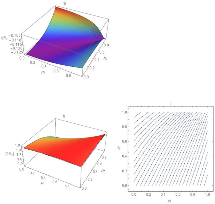
The gradient, the n partial derivatives of ℜ_v with respect to the p-variables, and the magnitude and direction of this vector-valued function. a) The ASRΔℜ_v approximates the change in ℜ_v at points (p₁, p₂) corresponding to increases in Δp₁ and Δp₂, here both equal to 0.05. The more negative the value of Δℜ_v, the larger the reduction. b) Lengths, |∇ℜ_v|, or magnitudes of the gradient (i.e., rates of change in ℜ_v) at points (p₁, p₂). c) Directions of the negative gradient ∇ℜ at evenly spaced points (p₁, p₂) where arrows indicate the changes in p₁ and p₂ that would yield the greatest reductions in ℜ_v. Equivalently, at any point (p₁, p₂), increasing p₁ and p₂ in the direction of ∇ℜ_v would most efficiently (i.e., require the fewest doses of vaccine) achieve any particular Δℜ_v. See the text for derivation. Other parameter values are ε₁ = 0.3, ε₂ = 0.1, a₁ = 5, a₂ = 10, N₁ = 750, and N₂ = 250.

3.7 Targeting Vaccination

The gradient provides a means of identifying which sub-population to vaccinate to affect ℜ_v the most. Figure 6a illustrates the Δℜ_v corresponding to Δp₁ and Δp₂ of 5%. Figures 6b and c illustrate the magnitudes of the vector, ∇ℜ_v and directions of the negative gradient at each point, respectively. We observe that different trajectories follow the gradient depending on starting point. Near the point p₁ = 1 and p₂ = 0, the arrow is almost vertical (i.e., the gradient direction has only a small p₁ component), indicating that changes in p₂ would affect ℜ_v the most.

In the example of Fine et al. (17), sub-population contact rates different considerably. For illustrative purposes, let a₁ = 15 and a₂ = 12 so that ℜ₀₁ = 5 and ℜ₀₂ = 4 (the values of β and γ are the same as before, i.e., β = 0.05 and γ = 0.15). If ε₁ = ε₂ = 1, then for all (p₁, p₂) with p₂ > (5/4) p₁ − 1/4, we have that ℜ_v = ℜ_v1 = 5(1 − p₁), which implies that the gradient direction is horizontal; thus, only population 1 need be vaccinated to attain ℜ_v = 1. However, this is true only when sub-populations are isolated. For example, let ε₁ = ε₂ = 0.3, N₁ = 1100, and N₂ = 900. In this case, illustrated in figure 7a, we observe that the gradient is neither horizontal nor vertical for any (p₁, p₂). We observe also that the trajectories in the p₁-p₂ plane, when the gradient direction is followed, are not straight lines, as shown in figure 7b. While this may be perfectly obvious when n = 2, meta-populations generally comprise many more or less interconnected sub-populations.

Figure 7.

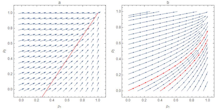
The a) negative gradient ∇ℜ at evenly spaced points (p₁, p₂) and b) optimal path from arbitrary starting points for a modification of the example of Fine et al. solely to increase transparency. The arrows in figure 7a, a vector plot, indicate the changes in p₁ and p₂ that would yield the greatest reductions in ℜ_v, represented by their sizes, while those in figure 7b, a stream plot, indicate only direction. Because these two sub-populations are not isolated, the gradient is defined over the entire parameter space. And, because their contact rates are not as disparate as those of Fine et al., the gradient directions do not seem to be either horizontal or vertical.

3.8 Optimal Vaccine Coverage

The gradient also describes the most efficient means of attaining any programmatic goal: To illustrate this, we fix Δℜ_v (i.e., the amount by which ℜ_v is to be reduced). Without loss of generality, we assume that Δℜ_v is small (or that the prescribed reduction of Δℜ_v is a sum of small increments) and denote the gradient vector at the point (p_1c, p_2c) by ∇ℜ_v = (v_1c, v_2c).

If we increase the fractions immune by Δp₁ and Δp₂ along a unit direction, u⃗ = (a,b), then (Δp₁, Δp₂) = ru⃗, where r is a constant determining the magnitude of the vector (Δp₁, Δp₂). It follows that Δℜ_v ≈ (v_1c,v_2c)·(ru⃗), so that |Δℜ_v| ≈ r|(v_1c,v_2c)| × | cos Θ |, where Θ is the angle between the gradient vector at (p₁, p₂) and the unit length vector u⃗. Note that the expression |(v_1c, v_2c)| × | cos Θ | is largest when |cos Θ| = 1 (i.e., when Θ = π, because ∂ℜ_v/∂p_i < 0). Thus, the value r is minimized when u⃗ is parallel to the gradient vector (v_1c,v_2c); that is, u⃗ = (v_1c,v_2c)/|(v_1c,v_2c)|. Thus, (Δp₁, Δp₂) ≈ r(v_1c, v_2c)/|(v_1c, v_2c)|, whereupon Δp₁N₁ + Δp₂N₂ ≈ r(v_1cN₁ + v_2cN₂)/| (v_1c, v_2c)|. Therefore, the increase in doses Δp₁N₁ + Δp₂N₂ is smallest when the vector (Δp₁,Δp₂) is parallel to the gradient vector ∇ℜ_v at the point (p_1c, p_2c). Goldstein et al. (25) consider the similar problem of the ∇ℜ_v that could be attained by optimally allocating a fixed amount of vaccine.

The gradient can also be used to devise optimal allocation strategies for limited vaccines. We can minimize ℜ_v(p₁, p₂) for fixed total vaccine doses p₁N₁ + p₂N₂ = c, where c > 0 is a constant representing the doses available, with N₁ and N₂ being fixed constants. In this case, we solve the equation ∇ℜ_v +λ(N₁, N₂) = 0, subject to p₁N₁ + p₂N₂ = c, where λ is the Lagrange multiplier. Notice that the constraint corresponds to a line whose equation is p₂ = (c − p₁N₁)/N₂. As this line is orthogonal to ∇ℜ_v at the solution point (p₁, p₂), its intersection with the contour curve ℜ_v(p₁, p₂) to which it is tangent (figure 8) is the optimal vaccination program. Thus, for this set of parameter values and constraint, p₁ = 0.66 and p₂ = 0.29 reduces ℜ₀ = 4.6 (when p₁ = p₂ = 0) to ℜ_v = 2.2.

4. Discussion

Using the simplest meta-population model that is capable of informing vaccination policy, we reproduce earlier results concerning the effect of heterogeneity in inter-personal contact rates – attributable, for example, to disparate sub-population densities – on the basic meta-population reproduction number. We observe that this reasoning extends to any variable affecting sub-population reproduction numbers. Preferential mixing, especially if heterogeneous, also affects the basic meta-population reproduction number. We refine earlier results on effects of heterogeneity in sub-population immunities and preferential mixing on the effective meta-population reproduction number. Heterogeneity in immunity can result from disparate socioeconomic circumstances, religious or philosophical beliefs, or information about the risks and benefits of vaccination, to name but a few possible causes.

4.1 Theory

Were populations proportionally-mixing or homogeneous, the population-immunity threshold would inform vaccination programs to mitigate the risk of outbreaks upon the introduction of infectious people. For diseases that had been eliminated domestically, these would be travelers infected abroad. This threshold is defined as the immunity at which an average infectious person infects only one susceptible person.

If individuals differed only in the sizes of their sub-populations, one could use the meta-population reproduction number to determine a single population-immunity threshold, as Goldstein et al. (18) do on their page 20. But, when populations are either heterogeneous in characteristics affecting basic reproduction numbers (glossary, ℜ_0i) or sub-population members mix preferentially (glossary, 0 < ε_i ≤ 1), sets of sub-population immunities (i.e., pairs if there are only two sub-populations, triplets if there are three, and so on) satisfy the condition that only one susceptible person is infected per infectious person. Unless sub-populations are identical in characteristics affecting their basic reproduction numbers and their members mix proportionally, these sets cannot simply be averaged for comparison with overall or weighted average sub-population immunities, as is current public health practice.

Meta-population reproduction numbers (glossary, ℜ₀, ℜ_v) account for heterogeneity and preferential mixing, inevitable in spatial meta-populations inasmuch as proximity affects contacts. If effective meta-population reproduction numbers – average numbers of secondary infections per infectious person – exceed, equal or are less than one, the numbers of infected people will increase, remain the same, or diminish, respectively. Thus, vaccination programs designed to mitigate the risk of outbreaks should maintain effective meta-population reproduction numbers less than one.

4.1 Practice

Our first result of programmatic import is that, in assessing the impact of heterogeneity, one cannot ignore mixing. Mixing not only modifies the effects of heterogeneity, but identifies relevant sub-populations (i.e., mixing is proportional within and preferential between them). While others have recognized its importance (9-12), mixing has only recently begun being measured (26-28). However, geospatial location devices and proximity detectors promise to dramatically increase our understanding of the contact patterns by which the pathogens causing infectious diseases in host meta-populations are transmitted.

Our second such result is that differences among sub-populations in characteristics affecting their basic reproduction numbers – heterogeneity – may substantially increase meta-population reproduction numbers, especially when combined with preferential mixing. Sub-population members can differ, but not in these characteristics. We began by questioning whether sub-populations themselves were needed. In reaching this conclusion, we extend the contributions of many authors, some of whom studied characteristics affecting basic reproduction numbers (3-6) and others immunity (13-16), the additional characteristic affecting effective reproduction numbers.

Our third result of programmatic import is the gradient, a fundamentally new tool for exploring the combined effects of heterogeneity in characteristics affecting sub-population reproduction numbers and mixing among the members of different sub-populations on the average number of secondary infections per infectious person. The gradient evaluated at the point (p₁,…, p_n) is a vector giving the direction in which to move away from (p₁,…, p_n) so as to achieve the greatest change in ℜ_v.

We demonstrate that, at any point in the n-dimensional space described by sub-population immunities, increasing them in direction of the negative gradient would most efficiently (i.e., use the fewest doses of vaccine) achieve any desired reduction in the average number of secondary infections per infectious person. This belies Keeling's and Rohani's (24) assertion that “only for the very simplest of models can the calculation of optimal targeting be performed analytically,” providing an alternative to Medlock and Galvani's (29) simulation of an age-structured population model with different vaccine allocations and comparison of cases or death averted.

Highlights.

• Population-immunity thresholds are useful only in homogeneous, proportionally-mixing populations

• Meta-population effective reproduction numbers, ℜ_v, and related quantities always are useful

• Heterogeneity in variables affecting sub-population reproduction numbers is relevant

• Together with preferential mixing among sub-populations, such heterogeneity increases ℜ_v

• The vector of partial derivatives of ℜ_v with respect to sub-population immunities indicates which sub-populations to vaccinate to reduce ℜ_v most effectively and efficiently

Glossary

S_i, I_i, R_i, N_i

Numbers susceptible; numbers infected/infectious; numbers recovered/immune; total number in group (or sub-population) i

μ, γ

Specific (or per capita) birth/death and recovery rates

λ_i

Force (or hazard rate) of infection per susceptible member of group (or sub-population) i, a function defined in the text

n

Number of groups (or sub-populations), indexed by i, j, or k

a_i, β

Activity (average per capita contact rate) of people in group i; probability of infection, if susceptible, upon contact with an infectious person

c_ij

Mixing (or proportion of the contacts of members of group i that are with members of group j), a function defined in the text

I_j/N_j

Probability that a proportionally contacted member of group j is infected/infectious

f_j

Proportional (or activity-weighted proportional) mixing, a function defined in the text

ε_i

Preference (average fraction of contacts reserved for others in one's own group)

δ_ij

Kronecker delta, equal to 1 when i = j and 0 otherwise

∀i, ∃j

For all groups i; there is a group j

ℜ₀, ℜ_0i, ℜ_v, ℜ_vi

Overall and group-specific intrinsic (or basic) reproduction numbers, functions defined in the text; Overall and group-specific effective (or control by vaccination, hence the subscript v) reproduction numbers, functions defined in the text

p_i, p_c

Proportion of group i that has been immunized (proportion vaccinated × vaccine efficacy), proportion immunized at which ℜ_v = 1

A, B, C, D

Symbols defined in the text solely to simplify notation

ℜ̄₀

Average of ℜ_0i

m, σ²

Mean and variance of a_i

∂ℜ₀/∂ε_i ∂ℜ_v/∂p_i

Partial derivatives of the basic reproduction number with respect to preference and the control reproduction number with respect to immunity

∇R_v

Gradient, a vector function defined in the text

|∇ℜ_v|

Magnitude of the gradient

Appendix 1

Given that N = S + I + R, we can eliminate one equation.

Letting

$$\begin{array}{c}{x}_i=\frac{S_i}{N_i},y_i=\frac{I_i}{N_i},i=1,2\\ x_1^{\prime }=\mu (1-p_1)-({\lambda }_1+\mu )x_1\\ x_2^{\prime }=\mu (1-p_2)-({\lambda }_2+\mu )x_2\\ y_1^{\prime }={\lambda }_1{x}_1-(\gamma +\mu )y_1\\ y_2^{\prime }={\lambda }_2{x}_2-(\gamma +\mu )y_2\\ {\lambda }_i=a_i\beta {\sum }_j{c}_{ij}{y}_j\end{array}$$

At the disease-free equilibrium, x_i = 1 − p_i, i = 1,2

Substituting,

$$\begin{array}{c}{y}_1^{\prime }=(a_1{c}_{11}\beta y_1+a_1{c}_{12}\beta y_2)(1-p_1)-(\gamma +\mu )y_1=f_1(y_1,y_2)\\ y_2^{\prime }=(a_2{c}_{21}\beta y_1+a_2{c}_{22}\beta y_2)(1-p_2)-(\gamma +\mu )y_2=f_2(y_1,y_2)\end{array}$$

The Jacobian, $J={\left(\begin{array}{cc}\frac{\partial f_1}{\partial y_1}& \frac{\partial f_1}{\partial y_2}\\ \frac{\partial f_2}{\partial y_1}& \frac{\partial f_2}{\partial y_2}\end{array}\right)}_{(y_1=0,y_2=0)}=\left(\begin{array}{cc}{a}_1{c}_{11}\beta (1-p_1)-(\gamma +\mu )& a_1{c}_{12}\beta (1-p_1)\\ a_2{c}_{21}\beta (1-p_2)& a_2{c}_{22}\beta (1-p_2)-(\gamma +\mu )\end{array}\right)$

We can rewrite J as F-V, where F are infection and V other terms

$$J=\left(\begin{array}{cc}{a}_1{c}_{11}\beta (1-p_1)& a_1{c}_{12}\beta (1-p_1)\\ a_2{c}_{21}\beta (1-p_2)& a_2{c}_{22}\beta (1-p_2)\end{array}\right)-\left(\begin{array}{cc}(\gamma +\mu )& 0\\ 0& (\gamma +\mu )\end{array}\right)$$

The next-generation matrix K = FV^–1

$$K=\left(\begin{array}{cc}{a}_1{c}_{11}\beta (1-p_1)& a_1{c}_{12}\beta (1-p_1)\\ a_2{c}_{21}\beta (1-p_2)& a_2{c}_{22}\beta (1-p_2)\end{array}\right)\times \left(\begin{array}{cc}\frac{1}{(\gamma +\mu )}& 0\\ 0& \frac{1}{(\gamma +\mu )}\end{array}\right)=\left(\begin{array}{cc}\frac{a_1{c}_{11}\beta (1-p_1)}{(\gamma +\mu )}& \frac{a_1{c}_{12}\beta (1-p_1)}{(\gamma +\mu )}\\ \frac{a_2{c}_{21}\beta (1-p_2)}{(\gamma +\mu )}& \frac{a_2{c}_{22}\beta (1-p_2)}{(\gamma +\mu )}\end{array}\right)=\left(\begin{array}{cc}{\Re }_{01}(1-p_1)c_{11}& {\Re }_{01}(1-p_1)c_{12}\\ {\Re }_{02}(1-p_2)c_{21}& {\Re }_{02}(1-p_2)c_{22}\end{array}\right)=\left(\begin{array}{cc}{\Re }_{v1}{c}_{11}& {\Re }_{v1}{c}_{12}\\ {\Re }_{v2}{c}_{21}& {\Re }_{v2}{c}_{22}\end{array}\right)$$

The reproduction number is the dominant eigenvalue of K.

Appendix 2

We restrict calculations in the main text to n = 2 because analytical expressions become unwieldy for n > 2 and some impossible for n > 4 and because graphing numerical solutions as functions of sub-population-specific quantities is difficult when n > 2. Most importantly, however, we doubt that any new ideas emerge when n > 2. When n = 3, for example, the next generation matrix is

$$K_3=\left[\begin{array}{ccc}{\mathrm{R}}_{v1}{c}_{11}& {\mathrm{R}}_{v1}{c}_{12}& {\mathrm{R}}_{v1}{c}_{13}\\ {\mathrm{R}}_{v2}{c}_{21}& {\mathrm{R}}_{v2}{c}_{22}& {\mathrm{R}}_{v2}{c}_{23}\\ {\mathrm{R}}_{v3}{c}_{31}& {\mathrm{R}}_{v3}{c}_{32}& {\mathrm{R}}_{v3}{c}_{33}\end{array}\right].$$

The characteristic equation is

$${\lambda }^3-\text{Tr}(K_3){\lambda }^2+q\lambda -\text{det}(K_3)=0,$$

where

$$q={\mathrm{R}}_{v1}{c}_{11}{\mathrm{R}}_{v2}{c}_{22}+{\mathrm{R}}_{v1}{c}_{11}{\mathrm{R}}_{v3}{c}_{33}+{\mathrm{R}}_{v2}{c}_{22}{\mathrm{R}}_{v3}{c}_{33}-{\mathrm{R}}_{v1}{c}_{12}{\mathrm{R}}_{v2}{c}_{21}-{\mathrm{R}}_{v1}{c}_{13}{\mathrm{R}}_{v3}{c}_{31}-{\mathrm{R}}_{v2}{c}_{23}{\mathrm{R}}_{v3}{c}_{32}.$$

And ℜ_v is the largest eigenvalue of the characteristic equation.

Consider ℜ_v as a function of p₁, p₂ and p₃ with all other parameter values fixed. Figure A1 shows the contour plot of ℜ_v for preferential (ε⃑ > 0, see A) and proportional mixing (ε⃑ = 0, see B). Plot C superimposes plots A and B to illustrate that, when mixing is preferential, higher vaccination coverage would be required to achieve ℜ_v < 1. Figure A2 shows three surfaces, corresponding to ε = 0, 0.4, and 0.8 (from bottom to top). The rectangular parallelepiped bounded by a red surface within which ℜ_v < 1 corresponds to the rectangle when n = 2 in manuscript figures 4.

Figure A1.

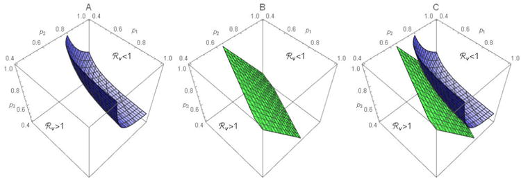
Contour surfaces for 3 sub-groups when mixing is preferential (A) or proportional (B). Plot C superimposes the surfaces in A and B. Parameter values are a₁ = 8, a₂ = 12, a₃ = 10, N₁ = N₂ = N₃ = 500, and ε₁ = ε₂ = ε₃ = ε with ε = 0.4 in A and ε = 0 in B.

Figure A2.

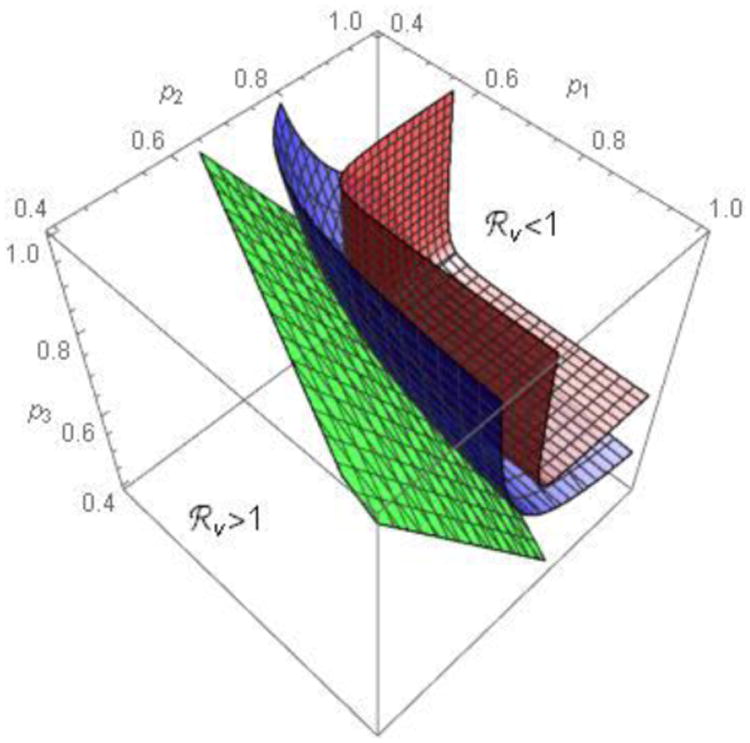
Contour surfaces for 3 sub-populations. The surfaces are for ε⃑ = 0 (bottom), ε⃑ = 0.4 (middle) and ε⃑ = 0.8 (top). Other parameter values are the same as in Figure A1.

Appendix 3

To prove (i), notice that when ε₁ = ε₂ = 0, we have

$$c_{11}=c_{21}=\frac{a_1{N}_1}{a_1{N}_1+a_2{N}_2}=\frac{a_1}{a_1+a_2},c_{22}=c_{12}=\frac{a_2{N}_2}{a_1{N}_1+a_2{N}_2}=\frac{a_2}{a_1+a_2}.$$

Thus,

$${\mathrm{R}}_0=\frac{\beta }{\gamma +\mu }\left(\frac{a_1^2+a_2^2}{a_1+a_2}\right).$$

Let a₂ = a_T − a₁ and let

$$F(a_1)=\frac{a_1^2+a_2^2}{a_T}=\frac{a_1^2+{(a_T-a_1)}^2}{a_T}.$$

Then ℜ₀ = F(a₁)β/(γ + μ). Note that F(a₁) is a decreasing (increasing) function on 0 < a₁ < a_T (a_T/2 < a₁ < a_T) and that F(0) = F(a_T). That is, F(a₁) has a minimum at a₁ = a_T/2, and it achieves its maximum at a₁ = 0 and a₁ = a_T . Therefore, ℜ₀(0,0) is minimized when a₁ = a₂, and maximized when a₁ = 0 and a₁ = a_T.

To prove (ii), notice that for ε₁ = 1 or ε₂ = 1 we have c₁₁ = c₂₂ = 1 and c₁₂ = c₂₁ = 0. Therefore, ℜ₀(ε₁,1) = ℜ₀(1, ε₂) = max{ℜ₀₁,ℜ₀₂}. It is easy to see that max{ℜ₀₁,ℜ₀₂} is the smallest when a₁ = a₂ = a_T/2, and the largest when a₁ = 0 (in which case ℜ₀ = ℜ₀₂ = βa_T/(γ + μ)) or when a₁ = a_T (in which case ℜ₀ = ℜ₀₁ = βa_T/(γ + μ)).

Together with the fact that ℜ₀(ε₁, ε₂) increases with ε₁ and ε₂ for all 0 < ε₁, ε₂ < 1, we would expect the behavior shown in figure 2 (i.e., the ℜ₀(ε₁, ε₂) surface moves up as heterogeneity in a increases).

References

- 1.Levins R. Some demographic and genetic consequences of environmental heterogeneity for biological control. Bulletin of the Entomological Society of America. 1969;15(3):237–40. [Google Scholar]
- 2.Ball F, Britton T, House T, et al. Seven challenges for meta-population models of epidemics, including household models. Epidemics. 2014 doi: 10.1016/j.epidem.2014.08.001. [DOI] [PubMed] [Google Scholar]
- 3.Dietz K. Models for vector-borne parasitic diseases. In: Barigozzi Claudio., editor. Vito Volterra Symposium on Mathematical Models in Biology Lecture Notes in Biomathematics. Vol. 39. 1980. pp. 264–77. [Google Scholar]
- 4.Anderson RM, Medley GF, May RM, et al. A preliminary study of the transmission dynamics of human immunodeficiency virus (HIV), the causative agent of AIDS. IMA J Math Appl Med Biol. 1986;3(4):229–63. doi: 10.1093/imammb/3.4.229. [DOI] [PubMed] [Google Scholar]
- 5.May RM, Anderson RM. The transmission dynamics of human immunodeficiency virus (HIV) Phil Trans R Soc Lond B. 1988;321(1207):565–607. doi: 10.1098/rstb.1988.0108. [DOI] [PubMed] [Google Scholar]
- 6.Diekmann O, Heesterbeek JAP, Metz JAJ. On the definition and the computation of the basic reproduction ratio ℜ0 in models for infectious diseases in heterogeneous populations. J Math Biol. 1990;28(4):365–82. doi: 10.1007/BF00178324. [DOI] [PubMed] [Google Scholar]
- 7.Nold A. Heterogeneity in disease transmission modeling. Math Biosci. 1980;52(3-4):227–40. [Google Scholar]
- 8.Jacquez JA, Simon CP, Koopman J, et al. Modeling and analyzing HIV transmission: the effect of contact patterns. Math Biosci. 1988;92(2):119–99. [Google Scholar]
- 9.Barbour AD. Macdonald's model and the transmission of bilharzias. Trans R Soc Trop Med Hyg. 1978;72(1):6–15. doi: 10.1016/0035-9203(78)90290-0. [DOI] [PubMed] [Google Scholar]
- 10.Dye C, Hasibeder G. Population dynamics of mosquito-borne disease: effects of flies which bite some people more frequently than others. Trans R Soc Trop Med Hyg. 1986;80(1):69–77. doi: 10.1016/0035-9203(86)90199-9. [DOI] [PubMed] [Google Scholar]
- 11.Hasibeder G, Dye C. Population dynamics of a mosquito-borne disease: persistence in a completely heterogeneous environment. Theor Popul Biol. 1988;33(1):31–53. doi: 10.1016/0040-5809(88)90003-2. [DOI] [PubMed] [Google Scholar]
- 12.Adler FR. The effects of averaging on the basic reproduction ratio. Math Biosci. 1992;111(1):89–98. doi: 10.1016/0025-5564(92)90080-g. [DOI] [PubMed] [Google Scholar]
- 13.May RM, Anderson RM. Spatial heterogeneity and the design of immunization programs. Math Biosci. 1984;72(1):83–111. [Google Scholar]
- 14.May RM, Anderson RM. Spatial, temporal and genetic heterogeneity in host populations and the design of immunization programmes. IMA J Math Appl Math Biol. 1984;1(3):233–66. doi: 10.1093/imammb/1.3.233. [DOI] [PubMed] [Google Scholar]
- 15.Hethcote HW. An immunization model for a heterogeneous population. Theor Popul Biol. 1978;14(3):338–49. doi: 10.1016/0040-5809(78)90011-4. [DOI] [PubMed] [Google Scholar]
- 16.Hethcote HW, van Ark JW. Epidemiological models for heterogeneous populations: proportionate mixing, parameter estimation and immunization programs. Math Biosci. 1987;84(1):85–118. [Google Scholar]
- 17.Fine P, Eames K, Heymann DL. “Herd Immunity”: a rough guide. Clin Infect Dis. 2011;52(7):911–16. doi: 10.1093/cid/cir007. [DOI] [PubMed] [Google Scholar]
- 18.Goldstein E, Paur K, Fraser C, Kenah E, Wallinga J, Lipsitch M. Reproductive numbers, epidemic spread and control in a community of households. Math Biosci. 2009;221:11–25. doi: 10.1016/j.mbs.2009.06.002. [DOI] [PMC free article] [PubMed] [Google Scholar]
- 19.van den Driessche P, Watmough J. Reproduction numbers and sub-threshold endemic equilibria for compartmental models of disease transmission. Math Biosci. 2002;180(1-2):29–48. doi: 10.1016/s0025-5564(02)00108-6. [DOI] [PubMed] [Google Scholar]
- 20.Diekmann O, Heesterbeek JAP, Roberts MG. The construction of next-generation matrices for compartmental epidemic models. J R Soc Interface. 2010;7(47):873–85. doi: 10.1098/rsif.2009.0386. [DOI] [PMC free article] [PubMed] [Google Scholar]
- 21.Chow L, Fan M, Feng Z. Dynamics of a multi-group epidemiological model with group-targeted vaccination strategies. J Theor Biol. 2011;291:56–64. doi: 10.1016/j.jtbi.2011.09.020. [DOI] [PubMed] [Google Scholar]
- 22.Colizza V, Vespignani A. Epidemic modeling in metapopulation systems with heterogeneous coupling pattern: theory and simulations. J Theor Biol. 2008;251:450–67. doi: 10.1016/j.jtbi.2007.11.028. [DOI] [PubMed] [Google Scholar]
- 23.Apolloni A, Poletto C, Ramasco JJ, Jensen P, Colizza V. Metapopulation epidemic models with heterogeneous mixing and travel behavior. Theor Biol Med Model. 2014;11:3. doi: 10.1186/1742-4682-11-3. [DOI] [PMC free article] [PubMed] [Google Scholar]
- 24.Keeling MJ, Rohani P. Modeling Infectious Diseases in Humans and Animals. Princeton Univ Press; 2007. [Google Scholar]
- 25.Goldstein E, Apolloni A, Lewis B, et al. Distribution of vaccine/antivirals and the ‘least spread line’ in a stratified population. J R Soc Interface. 2010;7:755–64. doi: 10.1098/rsif.2009.0393. [DOI] [PMC free article] [PubMed] [Google Scholar]
- 26.Del Valle SY, Hyman JM, Hethcote HW, et al. Mixing patterns between age groups in social networks. Soc Networks. 2007;29(4):539–54. [Google Scholar]
- 27.Mossong J, Hens N, Jit M, et al. Social contacts and mixing patterns relevant to the spread of infectious diseases. PLoS Med. 2008;5(3):381–91. doi: 10.1371/journal.pmed.0050074. [DOI] [PMC free article] [PubMed] [Google Scholar]
- 28.Zagheni E, Billari FC, Manfredi P, et al. Using time-use data to parameterize models for the spread of close-contact infectious diseases. Am J Epidemiol. 2008;168(9):1082–90. doi: 10.1093/aje/kwn220. [DOI] [PubMed] [Google Scholar]
- 29.Medlock J, Galvani AP. Optimizing influenza vaccine distribution. Science. 2009;325(5948):1705–08. doi: 10.1126/science.1175570. [DOI] [PubMed] [Google Scholar]