Fitting dynamic models to epidemic outbreaks with quantified uncertainty: A primer for parameter uncertainty, identifiability, and forecasts

Abstract

Mathematical models provide a quantitative framework with which scientists can assess hypotheses on the potential underlying mechanisms that explain patterns in observed data at different spatial and temporal scales, generate estimates of key kinetic parameters, assess the impact of interventions, optimize the impact of control strategies, and generate forecasts. We review and illustrate a simple data assimilation framework for calibrating mathematical models based on ordinary differential equation models using time series data describing the temporal progression of case counts relating, for instance, to population growth or infectious disease transmission dynamics. In contrast to Bayesian estimation approaches that always raise the question of how to set priors for the parameters, this frequentist approach relies on modeling the error structure in the data. We discuss issues related to parameter identifiability, uncertainty quantification and propagation as well as model performance and forecasts along examples based on phenomenological and mechanistic models parameterized using simulated and real datasets.

1. Introduction

Emerging and re-emerging infectious diseases are undoubtedly one of humankind’s most important health and security risks (Fauci & Morens, 2016). As epidemic threats increase so is the potential impact of mathematical and statistical inference and simulation approaches to guide prevention and mitigation plans. As the recent 2013–2016 Ebola epidemic exemplified, an infectious disease outbreak often forces public health officials to make key decisions to mitigate the outbreak in a changing environment where multiple factors positively or negatively impact local disease transmission (Chowell et al., 2017). Hence, public health officials are often interested in practical yet mathematically rigorous and computationally efficient approaches that comprehensively assimilate data and model uncertainty to 1) generate estimates of key transmission parameters, 2) assess the impact of control interventions (vaccination campaigns, behavior changes), 3) test hypotheses, 4) evaluate how behavior changes affect transmission dynamics, 5) gain insight to the contribution of different transmission pathways, 6) optimize the impact of control strategies, and 7) generate short and long-term forecasts, just to name a few.

Mathematical models provide a quantitative framework with which scientists can assess hypotheses on the potential underlying mechanisms that explain patterns in the observed data at different spatial and temporal scales. Models vary in their complexity in terms of the number of variables and parameters that characterize the dynamic states of the system, in their spatial and temporal resolution (e.g., discrete vs. continuous time), and in their design (e.g., deterministic or stochastic). While agent-based models, formulated in terms of characteristics and interactions among individual agents, have become increasingly used to model detailed processes often occurring at multiple scales (e.g., within host vs. population level), models based on systems of ordinary differential equations are widely used in the biological and social sciences. These dynamic models are specified by a set of equations and their parameters that together quantify the spatial-temporal states of the system via a set of interrelated dynamic quantities (e.g, viral load, susceptibility levels, disease prevalence) (Banks et al., 2009).

In this paper we review and illustrate a simple data assimilation framework for connecting ordinary differential equation models to time series data describing the temporal progression of case counts relating to population growth or infectious disease transmission dynamics (e.g, daily incident cases). This frequentist approach relies on modeling the error structure in the data unlike Bayesian approaches which always raise the question of how to set priors for the parameters. We present examples based on phenomenological and mechanistic models of disease transmission dynamics together with simulated and real datasets. We discuss issues related to parameter identifiability, uncertainty quantification and propagation as well as model performance and forecasts.

2. Mathematical models

The general form of a dynamic model composed by a system of $h$ ordinary differential equations is given by

$$\begin{array}{l}{\dot{x}}_1\left(t\right)=f_1(x_1,x_2,\dots ,x_h,\Theta )\\ {\dot{x}}_2\left(t\right)=f_2(x_1,x_2,\dots ,x_h,\Theta )\\ ⋮\\ {\dot{x}}_h\left(t\right)=f_h(x_1,x_2,\dots ,x_h,\Theta )\end{array}$$

where ${\dot{x}}_i$ denotes the rate of change of the system states $x_i$ where $i=\mathrm{1,2},\dots h$ and $\Theta =\left({\theta }_1,{\theta }_2,\dots ,{\theta }_m\right)$ is the set of model parameters.

In general, the complexity of a model is a function of the number of parameters that are needed to characterize the states of the system and the spectrum of the dynamics that can be recovered from the model (e.g., number of equilibrium points, oscillations, bifurcations, chaos). A trade-off exists between the level of model complexity and the ability to reliably parameterize the model with available data.

In the next sections we briefly discuss differences between phenomenological and mechanistic models along specific examples that will become useful to illustrate methodology in the subsequent sections.

2.1. Phenomenological models

Phenomenological models provide an empirical approach without a specific basis on the physical laws or mechanisms that give rise to the observed patterns in the data (Chowell et al., 2016a). Thus, these types of models emphasize the reproducibility of empirical observations using simple models. Next, we describe two useful models to characterize epidemic growth patterns namely the generalized-growth model (GGM) and the generalized Richards model (GRM).

2.1.1. The generalized-growth mode (GGM)

This is a phenomenological model that has proved useful to characterize and forecast early epidemic growth patterns (Chowell and Viboud, 2016, Viboud et al., 2016). In particular, previous analyses highlighted the presence of early sub-exponential growth patterns in infectious disease data across a diversity of disease outbreaks (Viboud et al., 2016). The generalized-growth model allows relaxing the assumption of exponential growth via a “scaling of growth” parameter, $p$. The model is given by the following differential equation:

$$C^{\prime }\left(t\right)=r{C}^p\left(t\right)$$ (1)

where $C^{\prime }\left(t\right)$ describes the incidence growth phase over time t, the solution $C\left(t\right)$ describes the cumulative number of cases at time t, $r$ is a positive parameter denoting the growth rate, and $p$, the “deceleration of growth” parameter varied between 0 and 1. If $p=0$, this equation describes constant incidence over time and the cumulative number of cases grows linearly while $p=1$ leads to the well-known exponential growth model (EXPM). Intermediate values of $p$ between 0 and 1 describe sub-exponential (e.g. polynomial) growth patterns. In semi-logarithmic scale, exponential growth patterns are visually evident when a straight line fits well several consecutive generations in the growth pattern, whereas a downward curvature in semi-logarithmic scale indicates early sub-exponential growth dynamics.

2.1.2. Generalized Richards model (GRM)

The GRM is an extension of the original Richards growth model (Richards, 1959) with three free parameters, which has been fitted to a range of logistic-type epidemic curves (Dinh et al, 2016, Hsieh and Cheng, 2006, Ma et al, 2014, Turner et al, 1976, Wang et al., 2012). When $C^{\prime }\left(t\right)$ represents the number of new infected cases at time $t$, the Richards model is given by the following differential equation:

$$C^{\text{'}}=rC\left[1-{\left(\frac{C}{K}\right)}^a\right]$$

where $r$ represents the intrinsic growth rate in the absence of any limitation to disease spread, $K$ is the size of the epidemic, and $a$ is a parameter that measures the extent of deviation from the S-shaped dynamics of the classical logistic growth model (Turner et al., 1976). During the early stages of disease propagation when $C\left(t\right)$ is significantly smaller than $K$, this model assumes an initial exponential growth phase. To account for initial sub-exponential growth dynamics (Viboud et al., 2016), we can modify the Richards model replacing the growth term $rC$ by $r{C}^p$ (Viboud et al., 2016), incorporating a ‘deceleration of growth’ parameter ($p$). Hence, the GRM has the form:

$$C^{\text{'}}=r{C}^p\left[1-{\left(\frac{C}{K}\right)}^a\right]$$ (2)

where $0\le p\le 1$. At the early stages of the epidemic, this model enables us to capture different growth profiles ranging from constant incidence ($p=0$), polynomial growth ($0<p<1$), to exponential growth ($p=1$) (Viboud et al., 2016). This model has been useful to generate post-peak forecasts of Zika and Ebola epidemics (Chowell et al., 2016b, Pell et al, 2016).

2.2. Mechanistic models

Mechanistic models incorporate key physical laws or mechanisms involved in the dynamics of the problem under study (e.g., population or transmission dynamics) in order to explain patterns in the observed data. This type of models are often formulated in terms of a dynamical system describing the spatial-temporal evolution of a set of variables and are useful to evaluate the emergent behavior of the system across the relevant space of parameters (Brauer & Nohel, 2012; Chowell et al., 2016a; Strogatz, 2014). In particular, compartmental models are based on systems of ordinary differential equations that focus on the dynamic progression of a population through different epidemiological states (Anderson and May, 1991, Bailey, 1975, Brauer, 2006, Lee et al., 2016). These models are useful to forecast prevalence levels in the short and long-term as well as assess the effects control interventions. In the context of disease transmission, population risk is typically modeled via a “transmission process” that requires contact between individuals or between an individual and external factors in the environment. Because the dynamic risk is limited to certain kinds of contact, the vast majority of epidemiological models divide the host population into different epidemiological states. Compartmental modeling allows researchers to address the conditions under which certain disease prevalence levels of interest will continue to grow in the population. Essentially this entails quantifying the factors that contribute to the “transmission” process. These models may be deterministic or stochastic, can incorporate geographic space, and can be structured by age, gender, ethnicity, or other risk groups (Sattenspiel, 2009). Such structuring is critical, since it defines discrete subgroups, or metapopulations, which may be considered networks wherein the populations are the nodes and their interconnections, the links.

2.2.1. The SEIR model

The simplest and most popular mechanistic compartmental model for describing the spread of an infectious agent in a well-mixed population is the SEIR (susceptible-exposed-infectious-removed) model (Anderson & May 1991). In this model, the infection rate is often defined as the product of three quantities: a constant transmission rate ($\beta$), the number of susceptible individuals in the population ($S\left(t\right)$), and the probability that a susceptible individual encounters an infectious individual ($\frac{I\left(t\right)}{N}$). Moreover, infected individuals experience a mean latent and a mean infectious period given by $1/k$ and $1/\gamma$, respectively. The model is based on a system of ordinary differential equations that keep track of the temporal progression in the number of susceptible (S), exposed (E), infectious (I), and removed (R) individuals as follows:

$$\begin{array}{l}\\ \{\begin{array}{l}\dot{S}=-\beta S\left(t\right)\frac{I\left(t\right)}{N}\\ \dot{E}=\beta S\left(t\right)\frac{I\left(t\right)}{N}-\kappa E\left(t\right)\\ \dot{I}=\kappa E\left(t\right)-\gamma I\left(t\right)\\ \dot{R}=\gamma I\left(t\right)\\ \dot{C}=\kappa E\left(t\right)\end{array}\end{array}$$

In the above system, $C\left(t\right)$ is an auxiliary variable that keeps track of the cumulative number of infectious individuals, and $\dot{C}\left(t\right)$ keeps track of the curve of new cases (incidence).

In a completely susceptible population, e.g., $S\left(0\right)\approx N$, the number of infectious individuals grows following an exponential function during the early epidemic growth phase, e.g., $I\left(t\right)\approx I_0{e}^{(\beta -\gamma )t}$ where the average number of secondary cases generated per primary case, $R_0$, is simply given by the product of the mean transmission rate ($\beta$) and the mean infectious period ($\frac{1}{\gamma }$) as follows: $R_0=\frac{\beta }{\gamma }$. However, as the number of susceptible individuals in the population declines due to a growing number of infections, the effective reproduction number over time, $R_t$, is given by the product of $R_0$ and the proportion of susceptible individuals in the population:

$$R_t=\frac{S\left(t\right)}{N}\frac{\beta }{\gamma }$$

3. The data

In order to calibrate mathematical models, researchers require time series data that describe the temporal changes in one or more states of the system. The temporal resolution of the data typically varies according to the time scale at which the relevant processes occur (e.g, daily, weekly, yearly) and the frequency at which the state of the system is measured. How well the model can be constrained to a given situation depends in part on the amount and resolution of the time series data. In general, we denote the time series of $n$ longitudinal observations by

$$y_{t_i}=y_{t_1},y_{t_1},\dots ,y_{t_n}\text{where}i=\mathrm{1,2},\dots ,n$$

where $t_i$ are the time points of the time series data and $n$ is the number of observations.

In our examples below, we make use of simulated data as well as outbreak data, which has been used in previous studies.

4. Sources of uncertainty

Parameter estimates for a given dynamical system are subject to two major sources of uncertainty:

• 1)Noise in the data which is typically addressed by assuming a particular error structure in the data, e.g., Poisson vs. negative binomial distribution; and
• 2)The underlying assumptions in the model employed for inferring parameter estimates from data.

Other sources of error could be associated with the algorithms employed to numerically solve the model in the absence of analytic or close-form solutions. Here we focus on quantifying parameter uncertainty arising from noise in the data.

5. Parameter estimation (nonlinear least squares fitting)

In the simplest manner, model parameters can be estimated via least-square fitting of the model solution to the observed data (Banks, Hu, & Thompson, 2014). This is achieved by searching for the set of parameters $\hat{\Theta }=\left({\hat{\theta }}_1,{\hat{\theta }}_2,\dots ,{\hat{\theta }}_m\right)$ that minimizes the sum of squared differences between the observed data $y_{t_i}=y_{t_1},y_{t_1},\dots ,y_{t_n}$ and the corresponding model solution denoted by $f(t_i,\Theta )$. That is, the objective function is given by

$$\hat{\Theta }=\arg \min \sum _{i=1}^n{(f(t_i,\Theta )-y_{t_i})}^2$$

where $t_i$ are the time points at which the time series data are observed, and $n$ is the number of data points available for inference. Hence, the model solution $f(t_i,\hat{\Theta })$ yields the best fit to the time series data $y_{t_i}$. However, it is important to keep in mind the underlying assumption in least squares fitting: the standard deviation of the errors (deviation of model to data) is invariant across the time series. In Matlab (The Mathworks, Inc.), two numerical optimization methods are available to solve the nonlinear least squares problem: The trust-region reflective algorithm and the Levenberg-Marquardt algorithm.

More generally, it is possible to simultaneously fit more than one state variable to their corresponding observed time series.

5.1. Weighted nonlinear least squares fitting

When each data point should not be given equal weight in the estimation of model parameters, weighted least squares can be useful to assign relative weights to each data point in our dataset. For instance, weights could reflect variable quality (e.g., precision of the measurements) of the time series so that less weight is given to those data points associated with inferior quality or precision. We define the nonnegative weights given to each data point as $w_{t_i}$ so that the objective function for weighted least squares fitting is given by

$$\hat{\Theta }=\arg \min \sum _{i=1}^n{w}_{t_i}{(f(t_i,\Theta )-y_{t_i})}^2$$

If we want to give more weight to smaller data points, the weights given to each data point can be modeled as follows:

$$w_{t_i}=1/y_{t_i}$$

If the goal is to give more weight to the most recent data, simple exponential smoothing can be used to assign higher weights to more recent data points relative to older data points. Specifically, the weights assigned to observations decrease exponentially as we move from recent to older data in the time series. Thus, the corresponding weight for observation $t_i$ is given by:

$$w_{t_{n-i}}=\alpha {(1-\alpha )}^{i-1}\text{where}i=\mathrm{0,1,2}\dots n-1$$

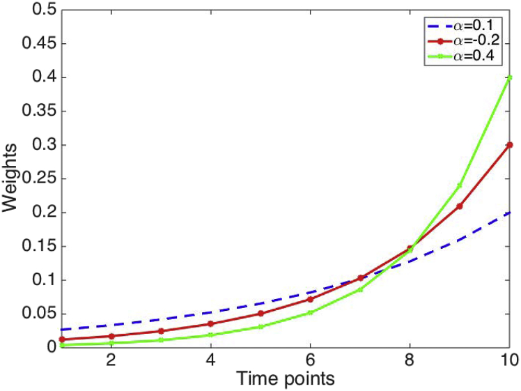
where parameter $0<\alpha <1$ regulate the rate at which the weights decrease exponentially so that the higher the value of alpha, the more weight is given to recent data relative to older data (Fig. 1).

Fig. 1.

Weight values according to simple exponential smoothing for various values of parameter $\alpha$ which regulate the rate at which the weights decrease exponentially. The higher the value of alpha, the more weight is given to recent data relative to older data.

6. Model diagnostics (residuals)

After parameters have been estimated, we can assess the quality of the model fit to the data by analyzing the temporal variation of the residuals, e.g., the difference between the best fit of the model and the time series data as a function of time:

$$\text{res}\left(t_i\right)=f(t_i,\hat{\Theta })-y_{t_i}$$

A random pattern in the temporal variation of the residuals suggests a good fit of the model to the data. Conversely, systematic deviations of the model to the data (e.g., temporal autocorrelation) indicate that the model deviates systematically from the data, which prompts modelers to reassess the current version of the model. If the model is used for forecasting purposes, it is particularly important that the residuals are uncorrelated and the variance of the residuals is approximately constant.

Example #1: Model fitting to time series data

The models:

The generalized-growth model (GGM)

The exponential growth model (EXPM)

The data:

We employ the weekly series of the number of reported Ebola cases in Sierra Leone during the 2014-16 Ebola epidemic in West Africa.

Parameter estimation:

We can fit the GGM to the first 15 weeks of the Ebola epidemic in Sierra Leone via least-square fitting using the Matlab built-in function lsqcurvefit.m. The initial number of cases $C\left(0\right)$ is fixed according to the first observation week in the data (i.e.,$C\left(0\right)=3$). The parameter estimates are as follows:

$$\begin{array}{l}r=0.81\hfill \\ p=0.48\hfill \end{array}$$

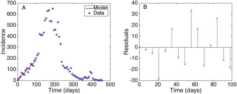
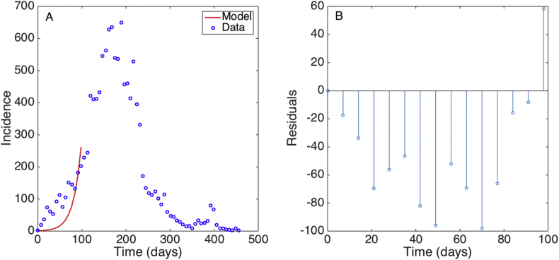
The best fit of the GGM model and the corresponding residuals using the first 15 weeks of data of the Ebola epidemic in Sierra Leone is shown in Fig. 2. Our estimate for the scaling of growth parameter $p$ indicates that the early growth pattern of the epidemic in Sierra Leone followed polynomial growth dynamics (Chowell et al., 2015). However, we still need to assess parameter uncertainty to construct confidence intervals and diagnose any potential parameter identifiability issues (see Section 9). While the GGM gives a good fit to the data, the EXPM model deviates systematically from the early growth phase, which is evident from the temporal autocorrelation in the set of residuals (Fig. 3).

Fig. 2.

A) The best fit of the GGM model to the first 15 weeks of the Ebola epidemic in Sierra Leone. The blue circles are the weekly case series while the solid red line corresponds to the best fit of the GGM to the data. B) the random pattern of the residuals as a function of time suggest that the model provides a reasonably good fit to the early growth phase of the epidemic.

Fig. 3.

A) The best fit of the EXPM model to the first 15 weeks of the Ebola epidemic in Sierra Leone. The blue circles are the weekly case series while the solid red line corresponds to the best fit of the EXPM to the data. B) the non-random pattern of the residuals is indicative of a systematic deviation of the model to the data.

Example #2: Weighted least squares fitting to time series data

The model:

The generalized-growth model (GGM)

Data weighting scheme:

Simple exponential smoothing.

Data:

We employ the weekly series of the number of reported Ebola cases in Sierra Leone during the 2014-16 Ebola epidemic in West Africa.

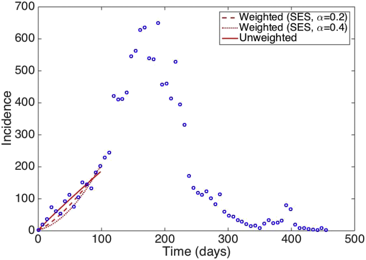
Best fits of the GGM to the first 15 weeks of the Ebola epidemic in Sierra Leone using weighted least square nonlinear fitting where the weights of the data points are assigned according to simple exponential smoothing are shown in Fig. 4.

Fig. 4.

Fits of the GGM model to the first 15 weeks of the Ebola epidemic in Sierra Leone using weighted least square nonlinear fitting where the weights of the data points are assigned according to simple exponential smoothing. The blue circles are the weekly case series while the solid, dashed, and dotted lines correspond to the best fits of the GGM to the data for various values of the parameter $\alpha$.

In the next section we present a computational approach for generating parameter uncertainty.

7. Parameter uncertainty

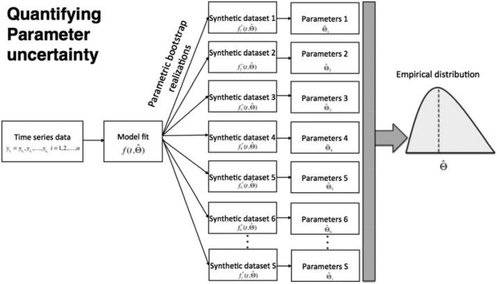
We rely on the general bootstrap method (Efron & Tibshirani, 1994) and describe a parametric bootstrapping approach which we have previously used in several publications to quantify parameter uncertainty and construct confidence intervals in mathematical modeling studies (e.g., (Chowell et al., 2006a, Chowell et al., 2006b)). In this method, multiple observations are repeatedly sampled from the best-fit model in order to quantify parameter uncertainty by assuming that the time series follow a Poisson distribution centered on the mean at the time points $t_i$. However, it is also possible to consider overdispersion in the data (see next section). This computational method requires generating simulated data from $f(t_i,\hat{\Theta })$, which is the best fit of the model to the data. The step-by-step algorithm to quantify parameter uncertainty follows (Fig. 5):

• 1.Derive the parameter estimates $\hat{\Theta }=\left({\hat{\theta }}_1,{\hat{\theta }}_2,\dots ,{\hat{\theta }}_m\right)$ through least-square fitting the model $f(t_i,\Theta )$ to the time series data $y_{t_i}=y_{t_1},y_{t_1},\dots ,y_{t_n}$to obtain the best-fit model, $f(t_i,\hat{\Theta })$.
• 2.Using the best-fit model $f(t_i,\hat{\Theta })$, we then generate S-times replicated simulated datasets, which we denote by $f_1^{\ast }(t_j,\hat{\Theta }),f_2^{\ast }(t_j,\hat{\Theta }),\dots ,f_S^{\ast }(t_j,\hat{\Theta })$.
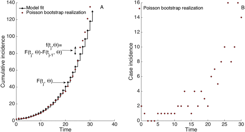
• 3.To generate the simulated datasets, we first use the best-fit model $f(t_i,\hat{\Theta })$ to calculate the corresponding cumulative curve function, $F^{\ast }(t_j,\hat{\Theta })$, as follows (see Fig. 6):

$$F(t_j,\hat{\Theta })=\sum _{l=1}^{j}f(t_l,\hat{\Theta })\text{where}j=\mathrm{1,2},\dots ,n$$

• 4.Each simulated dataset $f_k^{\ast }(t_j,\hat{\Theta })$ is generated by assuming a Poisson error structure as follows (Fig. 6):

$$f_k^{\ast }(t_j,\hat{\Theta })=\text{Po}(F(t_j,\hat{\Theta })-F(t_{j-1},\hat{\Theta }))\text{where}j=\mathrm{2,3},\dots ,n\text{and}k=\mathrm{1,2},\dots ,S$$

Fig. 5.

The parametric bootstrapping approach (Chowell et al., 2006a) generates multiple samples from the best-fit model in order to quantify the uncertainty of the parameter estimates. Briefly, we use$f(t_i,\hat{\Theta })$, the best fit of the model to the data to generate S synthetic datasets by assuming an error structure (e.g., Poisson or negative binomial). The S-simulated datasets are then given by $f_1^{\ast }(t_j,\hat{\Theta }),f_2^{\ast }(t_j,\hat{\Theta }),\dots ,f_s^{\ast }(t_j,\hat{\Theta })$. Next, parameters are re-estimated from each of the simulated datasets to derive a new set of parameter estimates denoted by ${\hat{\Theta }}_i$, where $i=\mathrm{1,2},\dots ,S$, with which we directly characterize parameter uncertainty (empirical parameter distributions), parameter correlations, and construct confidence intervals as well as generate forecasts of the system via uncertainty propagation in time.

Fig. 6.

Schematic diagram illustrates the parametric bootstrap approach for estimating parameter uncertainty (See also Fig. 5). Each bootstrap realization is simulated by assuming a Poisson error structure (or a negative binomial error structure) where the number of new case counts for each simulated dataset is computed using the increment in the number of case counts from time $t_{j-1}$ to $t_j$ (i.e. $F(t_j,\Theta )-F(t_{j-1},\Theta )$) as the Poisson mean for the number of new cases observed in the $t_{j-1}$ to $t_j$ interval (i.e., $\text{Po}(F(t_j,\Theta )-F(t_{j-1},\Theta ))$). A) Cumulative number of case counts. The solid black line corresponds to the known model solution while the red dots correspond to one simulated realization using the bootstrap approach. B) The corresponding number of new case counts (i.e., incidence) for one simulated realization.

Moreover, $f_k^{\ast }(t_1,\hat{\Theta })=f(t_1,\hat{\Theta })\text{for}k=\mathrm{1,2},\dots ,S.$ Thus, each new observation for each simulated dataset is sampled from a Poisson distribution (denoted by Po(.)) with mean $F(t_j,\hat{\Theta })-F(t_{j-1},\hat{\Theta })$.

• 5.Re-estimate parameters for each of the S-simulated realizations, which are given by ${\hat{\Theta }}_i$ where $i=\mathrm{1,2},\dots ,S.$
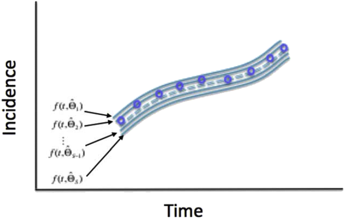
• 6.Using the set of re-estimated parameters (${\hat{\Theta }}_i$ where $i=\mathrm{1,2},\dots ,S$), it is possible to characterize their empirical distribution, correlations, and construct confidence intervals. The resulting uncertainty around the model fit is given by $f(t,{\hat{\Theta }}_1),f(t,{\hat{\Theta }}_2),\dots ,f(t,{\hat{\Theta }}_S)$ (Fig. 7).

Fig. 7.

Schematic diagrams illustrate the uncertainty around the model fit (blue lines) which is given by $f(t,{\hat{\Theta }}_1),f(t,{\hat{\Theta }}_2),\dots ,f(t,{\hat{\Theta }}_S)$ where the parameter uncertainty derived from our simulation study (described in Section 7) is given by ${\hat{\Theta }}_i$ where $i=\mathrm{1,2},\dots ,S$). The blue circles denote the time series data.

Example #2: Quantifying parameter uncertainty (see also Example #1)

Estimate the uncertainty of the $r\text{and}p$ parameters of the GGM calibrated to the early growth phase of the 2014-16 Ebola epidemic in Sierra Leone.

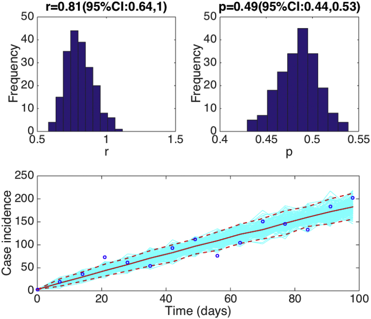
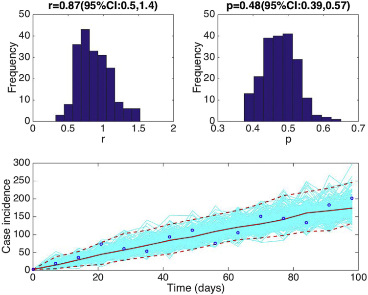
Assuming a Poisson error structure, Fig. 8 displays 1) the uncertainty of parameters “r” and “p” associated with the fit of the GGM model to the early phase of the Ebola epidemic in Sierra Leone and 2) the uncertainty in our parameter estimates translates into the 95% confidence bounds around the best fit of the model to the data.

Fig. 8.

Fitting the GGM to the first 15 weeks of the 2014-15 Ebola epidemic in Sierra Leone. Parameter estimates with quantified uncertainty generated using the methodology described in Section 7. The histograms display the empirical distributions of the parameter estimates using 200 bootstrap realizations. The bottom panel shows the fit of the GGM to the 15 weeks of the 2014-15 Ebola epidemic in Sierra Leone. The blue circles are the weekly data while the solid red line corresponds to the best fit of the GGM to the data. The blue lines correspond to 200 realizations of the epidemic curve assuming a Poisson error structure. The dashed red lines correspond to the 95% confidence bands around the best fit of the model to the data.

8. Data overdispersion

In the previous section we assumed a Poisson error structure to quantify parameter uncertainty. The Poisson distribution only requires one parameter and is suitable to model count data where the mean of the distribution equals the variance. In situations where the time series data shows overdispersion, we can employ a negative binomial distribution instead. The negative binomial distribution requires two parameters to model the mean and overdispersion in the data. Thus, it is possible to model variance levels in the data that are relatively higher than the mean.

Example #3: Quantifying parameter uncertainty with a negative binomial error structure (see also Example #2)

Assuming a negative binomial error structure where the variance is 5 times higher than the mean, we estimate the uncertainty of the $r\text{and}p$parameters of the GGM calibrated to the to the early growth phase of the 2014-16 Ebola epidemic in Sierra Leone. Results are shown in Fig. 9: 1) the uncertainty of parameters “r” and “p” associated with the fit of the GGM model to the early phase of the Ebola epidemic in Sierra Leone and 2) the 95% confidence bands around the best fit of the model to the data.

Fig. 9.

Fitting the GGM to the first 15 weeks of the 2014-15 Ebola epidemic in Sierra Leone. Parameter estimates with quantified uncertainty generated using the bootstrap approach with a negative binomial error structure with variance 5 times higher than the mean as described in the text (Section 7). The histograms display the empirical distributions of the parameter estimates using 200 bootstrap realizations. The bottom panel shows the fit of the GGM to the 15 weeks of the 2014-15 Ebola epidemic in Sierra Leone. The blue circles are the weekly data while the solid red line corresponds to the best fit of the GGM to the data. The dashed red lines correspond to the 95% confidence bands around the best fit of the model to the data. The confidence intervals of the parameter estimates are wider than those obtained using a Poisson error structure in the data (Fig. 8).

9. Parameter identifiability

A key question in model parameterization is whether the model parameters are identifiable from the available data. As a general rule, a parameter is identifiable when its confidence interval lies in a finite range of values (Cobelli and Romanin-Jacur, 1976, Jacquez, 1996, Raue et al, 2009). Conversely, lack of parameter identifiability can be recognized when large perturbations in the model parameters generate small changes in the model output (Capaldi et al, 2012, Chowell et al., 2006b, Pillonetto et al., 2003). Multiple factors can give rise to lack of parameter identifiability. For instance, structural parameter non-identifiability (Cobelli & Romanin-Jacur, 1976) results from the particular structure of the model independently of the characteristics of the observed time series data used to estimate parameters. However, even when structural identifiability is not an issue, a parameter may still be non-identifiable in practice due to other factors including: 1) the amount and quality of the data available and/or 2) the number of parameters that are jointly estimated from the available data. This type of parameter non-identifiability is commonly referred to as practical non-identifiability (Raue et al., 2009).

Structural parameter non-identifiability is often the most difficult to remedy as it requires appropriately modifying the model to eliminate the structural non-identifiability issue. On the other hand, practical parameter non-identifiability issues could be fixed by 1) employing an alternative model of lower complexity when possible, 2) collecting more data about other states in the system to better characterize the system dynamical features, 3) increasing the spatial-temporal resolution of the data to better constrain the model parameters and/or 4) reducing the number of parameters that are jointly estimated, perhaps by constraining a subset of the unknown parameters based on estimates previously reported in similar studies and conducting extensive sensitivity analyses on those parameters (Arriola et al., 2009). Finally, specific approaches have been adapted to address parameter identifiability including regularization techniques that aim for stable parameter reconstruction (Smirnova & Chowell, 2017).

Example #4: Parameter non-identifiability arises from the limited amount of data available to quantify parameter uncertainty

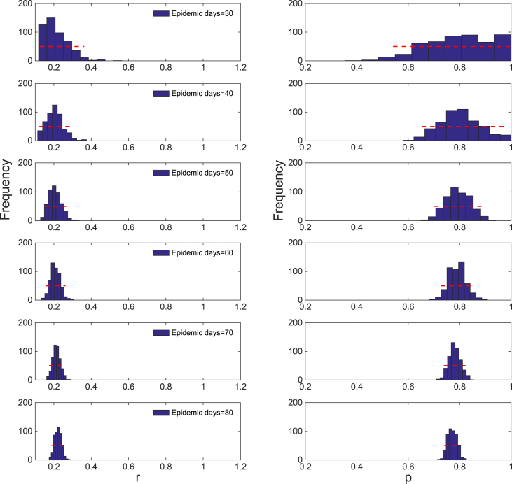
For this example, we first generate simulated data from the generalized-Richards model (GRM) using the parameter values: $r=0.2,p=0.8\text{,}a=1\text{,}\text{and}K=1000$. Next, we use the simulated data to attempt to estimate parameters $r\text{and}p$ using the GGM from an increasing length of the early growth phase of the daily incidence curve simulated using the GRM. Fig. 10 shows the resulting empirical distributions of the parameters using an increasing length of the growth phase: 10, 20, …, 80 days. Importantly, Fig. 10 shows that using only 10 days of data, it is not possible to reliably estimate the deceleration of growth parameter, $p$, because its confidence interval ranges widely from 0.5 to 1.0. Indeed, we conclude that it is not possible to discriminate between sub-exponential and exponential-growth dynamics based on data of only the first 10 days. In fact, the corresponding confidence interval of $p$ include the values of 0.5 and 1.0, which indicate that both linear and exponential growth dynamics cannot be ruled out with the data at hand. As more data of the early growth phase is employed to estimate parameters of the GGM, the uncertainty in parameter estimates is not only reduced, but the parameter estimates are better constrained around their true values (Fig. 10).

Fig. 10.

Empirical distributions of $r$ and $p$ of the GGM model derived from our bootstrap uncertainty method after fitting the GGM to an increasing length of the growth phase (10, 20, …, 80 days) of the daily incidence curve derived from the GRM model with parameters $r=0.2,p=0.8\text{,}a=1\text{,}\text{and}K=1000$. Importantly, using only 10 days of data, it is not possible to reliably estimate the deceleration of growth parameter, $p$, because its confidence interval ranges widely from 0.5 to 1.0. Indeed, it is not possible to discriminate between sub-exponential and exponential-growth dynamics based on data of only the first 10 days. However, as more data of the early growth phase is employed to estimate parameters of the GGM, the uncertainty in parameter estimates is not only reduced, but the parameter estimates are better constrained around their true values.

10. Parameter correlations

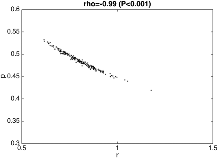
We can quantify the parameter correlations using our joint empirical distributions of the parameters (denoted by ${\hat{\Theta }}_i$where $i=\mathrm{1,2},\dots ,S$) which are derived from our bootstrap approach (described in Section 7)), For instance, for our Example # 2 based on fitting the GGM to the first 15 weeks of the Ebola epidemic in Sierra Leone, parameters ${\hat{r}}_i$ and ${\hat{p}}_i$ were significantly correlated as shown in Fig. 11. Despite this, the confidence intervals of these parameters display reasonable uncertainty to reliably characterize the parameters.

Fig. 11.

Correlation between ${\hat{r}}_i$ and ${\hat{p}}_i$ (where $i=\mathrm{1,2},\dots ,S$) derived from our parameter uncertainty method after fitting the GGM to the first 15 weeks of the Ebola epidemic in Sierra Leone.

Example #5: Evaluate the correlation of the $\hat{r},\hat{p}$ parameters derived from fitting the GGM to the first 15 weeks of the Ebola epidemic in Sierra Leone (See also Example #2; Fig. 11). These parameters are significantly correlated (Spearman rho = -0.99; P-value < 0.001).

11. Model selection (performance metrics)

While we can inspect the residuals for any systematic deviations of the model fit to the data, it is also possible to quantify the error of the model fit to the data using performance metrics (Kuhn & Johnson, 2013). These metrics are also useful to quantify the error associated with forecasts. A widely used performance metric is the root-mean- squared error (RMSE), which is given by

$$\text{RMSE}=\sqrt{\frac{1}{n}\sum _{i=1}^n{\left(f(t_i,\hat{\Theta })-y_{t_i}\right)}^2}$$

Another performance metric is the mean absolute error (MAE), which is given by

$$\text{MAE}=\frac{1}{n}\sum _{i=1}^n\left|f(t_i,\hat{\Theta })-y_{t_i}\right|$$

Similarly, the mean absolute percentage error (MAPE) is given by:

$$\text{MAPE}=\frac{1}{n}\sum _{i=1}^n\left|(f(t_i,\hat{\Theta })-y_{t_i})/y_{t_i}\right|$$

Example #6: Compare performance metrics for both the GGM and EXPM models when calibrated to the first 15 weeks of the 2014-16 Ebola epidemic in Sierra Leone (See also Example #1).

The RMSE, MAE, and MAPE of the fits provided by the GGM and EXPM models to the first 15 weeks of the Ebola epidemic in Sierra Leone (See also Fig. 2, Fig. 3) are as follows:

Model	RMSE	MAE	MAPE
GGM	16.91	13.67	0.16
EXPM	59.38	51.35	0.62

12. Model-based forecasts with quantified uncertainty

We are frequently interested in calibrating a model not only to understand and characterize the current state of the system, but also to aim to predict its behavior in the near or long terms. The particular time horizon of forecast depends on the purpose of the forecast. For instance, a long-term forecast (e.g., several years) could be useful to make strategic decisions regarding the construction of facilities to respond to natural disasters such as epidemics and hurricanes whereas a short-term forecast (e.g., days to weeks) are useful to plan for scheduling resources (e.g., number of face masks, hospital beds). However, it is important to keep in mind that forecasts are often inaccurate as these are mostly based on the current values and uncertainty of the parameters of the system, which are likely to change over time. Moreover, the further out the forecast is made, the more wrong it is expected to be.

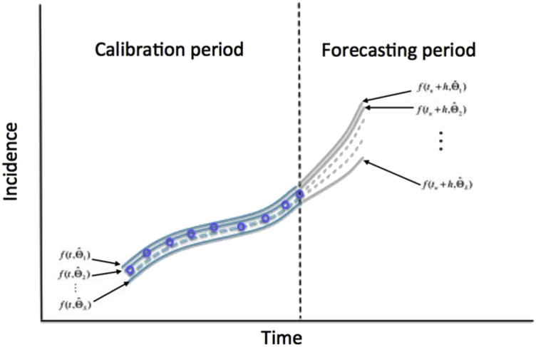
A properly calibrated model to data can be used to generate short-term or long-term forecasts of the system. Generating a forecast based on the model uncertainty given by $f(t,{\hat{\Theta }}_1),f(t,{\hat{\Theta }}_2),\dots ,f(t,{\hat{\Theta }}_S)$ is a relatively straightforward computational task that requires propagating the uncertainty of the current state of the system in time by a time horizon of $h$ time units as follows (see Fig. 12):

$$f(t+h,{\hat{\Theta }}_1),f(t+h,{\hat{\Theta }}_2),\dots ,f(t+h,{\hat{\Theta }}_S)$$

Fig. 12.

Schematic diagram shows the uncertainty around the model fit (blue lines; calibration period) given by $f(t,{\hat{\Theta }}_1),f(t,{\hat{\Theta }}_2),\dots ,f(t,{\hat{\Theta }}_S)$ and the corresponding uncertainty in the forecast for a time horizon of $h$ time units (gray lines; forecasting period) given by $f(t+h,{\hat{\Theta }}_1),f(t+h,{\hat{\Theta }}_2),\dots ,f(t+h,{\hat{\Theta }}_S)$. The blue circles denote the time series data. The vertical dashed line separates the calibration and forecasting periods.

That is, we forecast the entire uncertainty of the system using the uncertainty associated with the parameter estimates, which were previously derived from our uncertainty quantification procedure described in Section 7.

To assess forecasting performance, we can use one of the performance metrics (e.g., RMSE, MAE) previously described in Section 11.

Example #7: Forecast the early growth phase from daily synthetic data obtained from the GRM model.

The model:

The generalized-growth model (GGM)

The data:

Simulated daily incidence data using the generalized-Richards model (GRM) with parameters $r=0.2,p=0.8\text{,}a=1\text{,}\text{and}K=1000$.

Forecasts:

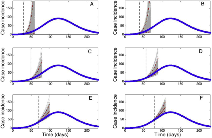
30-day ahead forecasts using the GGM by estimating parameters $r$ and $p$ with quantified uncertainty when the model is fitted to an increasing length of the epidemic growth phase (10, 20, …, 80 days) (Fig. 13).

Fig. 13.

30-day ahead forecasts derived using the GGM by estimating parameters$r$ and $p$ with quantified uncertainty when the model is fitted to an increasing length of the growth phase (10, 20, …, 80 days) of a synthetic daily incidence curve simulated using the GRM with parameters $r=0.2,p=0.8\text{,}a=1\text{,}\text{and}K=1000$. We can observe that the uncertainty of the forecasts narrows down as more data of the early growth phase is employed to estimate parameters of the GGM. That is, the uncertainty in parameter estimates is not only reduced, but the parameter estimates are also increasingly constrained around their true values (Fig. 8). Importantly, using only 10 days of data, it is not possible to reliably estimate discriminate between sub-exponential and exponential-growth dynamics. The cyan curves correspond to the uncertainty during the model calibration period while the gray curves correspond to the uncertainty in the forecast. The mean (solid red line) and 95% CIs (dashed red lines) of the model fit are also shown. The vertical line separates the calibration and forecasting periods.

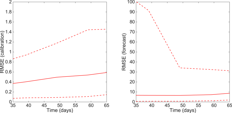
We can observe that the uncertainty of the forecasts narrows down as more data of the early growth phase is employed to estimate parameters of the GGM. That is, the uncertainty in parameter estimates is not only reduced, but the parameter estimates are also increasingly constrained around their true values (Fig. 13). Importantly, using only 10 days of data, it is not possible to reliably estimate discriminate between sub-exponential and exponential-growth dynamics. The corresponding performance of the GGM during the calibration and forecasting periods is shown in Fig. 14.

Fig. 14.

The root mean squared errors (RMSE) during the calibration and forecasting intervals using the generalized-growth model (GGM) when the model is fitted to an increasing length of the growth phase (10, 20, …, 80 days) of a synthetic daily incidence curve simulated using the GRM with parameters $r=0.2,p=0.8\text{,}a=1\text{,}\text{and}K=1000$. The mean (solid red line) and 95% CIs (dashed red lines) of the RMSE derived from the ensemble curves are shown (see Fig. 11 for the corresponding short-term forecasts).

Example #8: Forecast the early growth phase of the Zika epidemic in Antioquia, Colombia

The model:

The generalized-growth model (GGM)

The data:

The daily number of new Zika cases by date of symptoms onset in Antioquia, Colombia.

Forecasts:

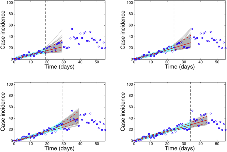
10-day ahead forecasts using the GGM by estimating parameters$r$ and $p$ with quantified uncertainty when the model is fitted to an increasing length of the epidemic growth phase (20, 25 30, 35 days) (Fig. 15).

Fig. 15.

10-day ahead forecasts provided by the generalized-growth model (GGM) when the model is fitted to an increasing amount of epidemic data: (A) 20, (B) 25, (C) 30, and (D) 35 epidemic days. The cyan curves correspond to the uncertainty during the model calibration period while the gray curves correspond to the ensemble of realizations for the model forecast. The mean (solid red line) and 95% CIs (dashed red lines) of the model fit are also shown. The vertical line separates the calibration and forecasting periods.

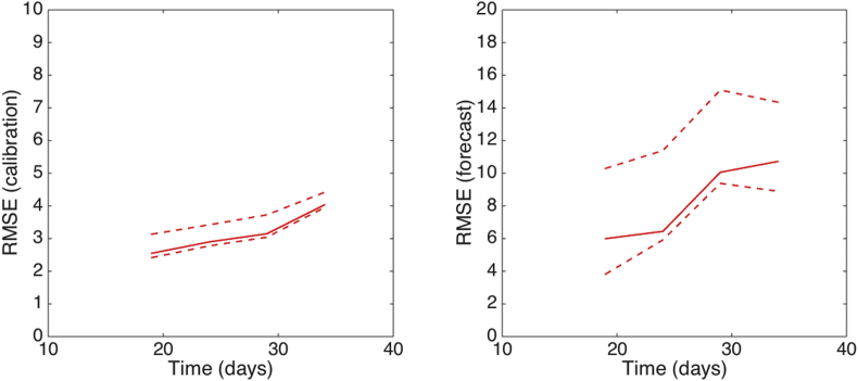
We can observe that the uncertainty of the forecasts narrows down as more data of the early growth phase is employed to estimate parameters of the GGM. Importantly, using less than 10 days of data, it is not possible to reliably estimate discriminate between sub-exponential and exponential-growth dynamics. The corresponding performance of the GGM during the calibration and forecasting periods is shown in Fig. 16 Matlab code for 1) fitting the GGM, 2) derive parameter uncertainty, and 3) generate short-term forecasts using incidence data of the Zika outbreak is provided in the supplement.

Fig. 16.

The root mean squared errors (RMSE) during the calibration and forecasting intervals using the generalized-growth model (GGM) when the model is fitted to an increasing amount of epidemic data of the Zika epidemic in Antioquia, Colombia: 20, 25, 30, 35 epidemic days. The mean (solid red line) and 95% CIs (dashed red lines) of the RMSE derived from the ensemble curves are shown (see Fig. 13 for the corresponding short-term forecasts).

Example #9: How much data is needed to refit a model to itself?

The model:

The generalized Richards model (GRM)

The data:

Simulated daily incidence data using the generalized-Richards model (GRM) with parameters $r=0.2,p=0.8\text{,}a=1\text{,}\text{and}K=1000$.

Forecasts:

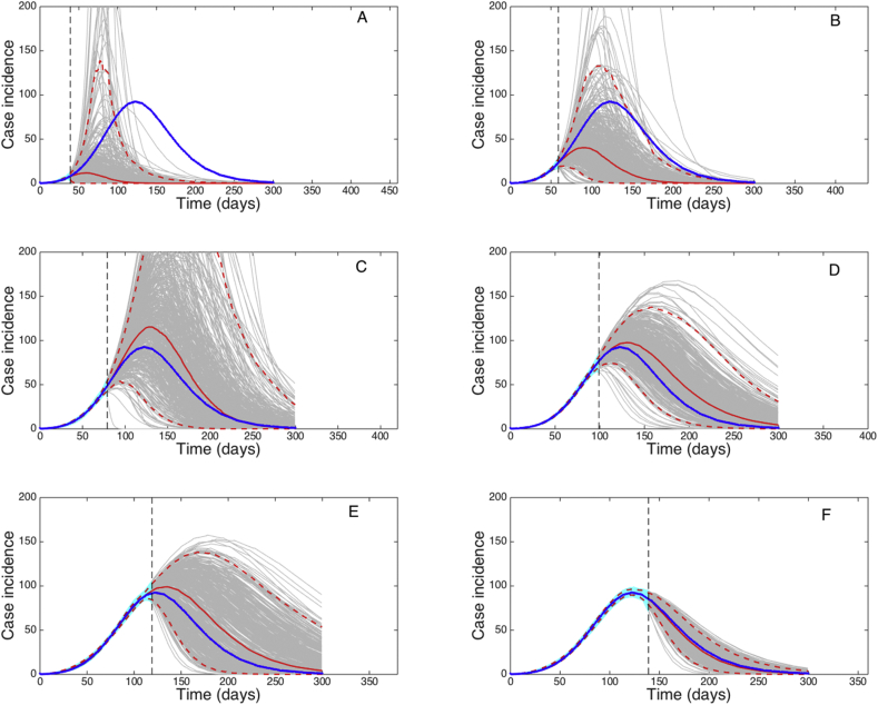
It is of interest to understand how much data is needed to faithfully calibrate a model to synthetic data derived from the same model. For this purpose, we conducted long-term forecasts based on the GRM, the same model that was employed to generate the data, by estimating parameters $r$,$p$ and $K$ using an increasing amount of epidemic data (40, 60, …, 140 days) (Fig. 17).

Fig. 17.

Long-term forecasts derived using the GRM by estimating parameters$r$, $p$ and $K$ with quantified uncertainty when the model is fitted to an increasing length of the growth phase (40, 60, …, 140 days) of a synthetic daily incidence curve simulated using the same GRM model with parameters $r=0.2,p=0.8\text{,}a=1\text{,}\text{and}K=1000$. Using only data of the early epidemic growth phase (before the inflection point occurring around day 50), the model is underdetermined and significantly underestimates the incidence curve. Forecasts are gradually improved particularly when the model is calibrated using data past the epidemic's inflection point. The cyan curves correspond to the uncertainty during the model calibration period while the gray curves correspond to the uncertainty in the forecast. The mean (solid red line) and 95% CIs (dashed red lines) of the model fit are also shown. The vertical line separates the calibration and forecasting periods.

Using only data of the early epidemic growth phase (before the inflection point occurring around day 50), the model is underdetermined and significantly underestimates the incidence curve. Forecasts are gradually improved particularly when the model is calibrated using data past the epidemic's inflection point (Fig. 17).

13. Quantifying uncertainty for composite parameters

In previous Examples #2 and #3, we measured the uncertainty of model parameters estimated from data by constructing confidence intervals using the empirical distribution of the parameters. However, it is possible to use the empirical distributions of the parameters to assess the uncertainty associated with composite parameters whose values depend on several existing model parameters and are often useful to gauge the behavior of the modeled system. For instance, a key epidemiological parameter to measure the transmissibility of a pathogen is the basic reproduction number, $R_0$ (Anderson and May, 1991, Diekmann et al., 1990, van den Driessche and Watmough, 2002). This parameter is a function of several parameters of the epidemic model including transmission rates and infectious periods of the epidemiological classes that contribute to new infections. This is an important parameter as it often serves as a threshold parameter for SEIR-type compartmental models. If $R_0>1$ then an epidemic is expected to occur whereas values of $R_0<1$cannot sustain disease transmission. For instance, for the simple SEIR model, the basic reproduction number is given by:

$$R_0=\frac{\beta }{\gamma }$$

Using the empirical distributions of the transmission rate (${\hat{\beta }}_i$ where $i=\mathrm{1,2},\dots ,S$) and the recovery rate (${\hat{\gamma }}_i$ where $i=\mathrm{1,2},\dots ,S$), we can directly estimate the empirical distribution of the basic reproduction number as follows (Chowell et al., 2006a, Chowell et al., 2009):

$${\hat{R}}_{0_i}=\frac{{\hat{\beta }}_i}{{\hat{\gamma }}_i}\text{where}i=\mathrm{1,2},\dots ,S$$

Using the empirical distribution of ${\hat{R}}_{0_i}$, we have full control of the uncertainty allowing us to not only construct confidence intervals, but also assess the probability that ${\hat{R}}_{0_i}$ lies above the epidemic threshold at 1.0.

Example #9: Estimating $R_0$ by fitting the SEIR model to the early epidemic growth phase (adapted from ref. (Chowell, Nishiura, & Bettencourt, 2007)).

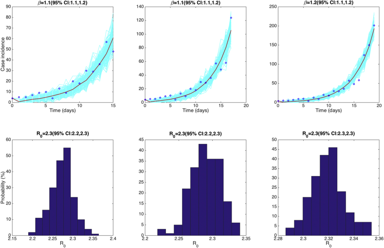
Here we provide an example of estimating $R_0$ of the 1918 influenza pandemic in San Francisco, California, by estimating the transmission rate $\beta$ while fixing the latent period at 2 days (e.g., $\kappa =1/2$) and the infectious period at 2 or 4 days (e.g., $\gamma =1/2$ or $\gamma =1/4$) based on the epidemiology of influenza.

The model:

SEIR model Chowell et al., 2007 described in Section 2.2.1

The data:

We employ the daily series of influenza case notifications during the fall wave of the 1918 influenza pandemic in San Francisco.

Baseline parameter values:

Latent period of 2 days (e.g., $\kappa =1/2$) while the infectious period was assumed to be 2 or 4 days (e.g., $\gamma =1/2$ or $\gamma =1/4$). At the time of the 1918 pandemic, San Francisco had a population size of approximately 550,000.

Parameter estimation:

For simplicity, we only estimate one parameter from the time series data of the early epidemic growth phase: the transmission rate, $\beta$. We can fit the SEIR to the first 16–20 days of the influenza pandemic in San Francsico via least-square fitting using the Matlab built-in function lsqcurvefit.m. The initial number of cases I(0) is fixed according to the first observation day in the data (i.e., C(0) = 4). For instance, fitting the model to the first 16 epidemic days, we estimate the transmission rate at:

$$\beta =1.1\left(95\text{\%}\text{CI:}1\text{.}1\text{,}1\text{.}2\right)$$

Uncertainty in $R_0$:

The best fit of the SEIR model to the first 16, 18, and 20 days of the influenza pandemic in San Francisco along the corresponding empirical distribution of $R_0$ is shown in Fig. 18. We can observe that the distribution of $R_0$ is stable when using 16, 18 or 20 epidemic days of data. $R_0$ was estimated at 2.3 (95% CI: 2.2, 2.3) using 16 epidemic days, 2.3 (95% CI: 2.2, 2.3) using 18 epidemic days, and 2.3 (95% CI: 2.3, 2.3) using 20 epidemic days.

Fig. 18.

Top panels show the best fit of the SEIR model and its uncertainty to the first 16, 18, and 20 days of data of the 1918 influenza pandemic in San Francisco. The blue circles are the weekly data while the solid red line corresponds to the best fit of the GGM to the data. The light blue lines correspond to 200 realizations of the epidemic curve assuming a Poisson error structure. The dashed red lines correspond to the 95% confidence bands around the best fit of the model to the data. Bottom panels display the normalized empirical distributions of $R_0$using the first 16, 18, or 20 days of the epidemic curve.

14. The effective reproduction number, $R_t$, with quantified uncertainty

While the basic reproduction number, commonly denoted by $R_0$, gauges the transmission potential of an infectious disease epidemic in a fully susceptible population during the early epidemic take off (Anderson & May 1982), the effective reproduction number $R_t$ captures changes in transmission potential over time (Chowell et al., 2016c, Nishiura et al., 2009). We can characterize the effective reproduction number and its uncertainty during the early epidemic exponential growth phase (Wallinga & Lipsitch, 2007). When the early dynamics follow sub-exponential growth, another method relies on the generalized-growth model (GGM) to characterize the profile of growth from early incidence data (Chowell et al., 2016c). In particular, the GGM can reproduce a range of growth dynamics from constant incidence ($p=0$) to exponential growth ($p=1$) (Viboud et al., 2016). We can generate the uncertainty associated with the effective reproduction number during the study period directly from the uncertainty associated with the parameter estimates $({\hat{r}}_i,{\hat{p}}_i)$ where $i=\mathrm{1,2},\dots ,S.$. That is, $R_{t_j}({\hat{r}}_i,{\hat{p}}_i)$ provides a curve of the effective reproduction number for each value of the parameters ${\hat{r}}_i,{\hat{p}}_i$where $i=\mathrm{1,2},\dots ,S.$ Then, we can compute the curves $R_{t_j}({\hat{r}}_i,{\hat{p}}_i)$ based on the incidence at calendar time $t_j$ denoted by $I(t_j,{\hat{r}}_i,{\hat{p}}_i)$, and the discretized probability distribution of the generation interval denoted by ${\rho }_{t_j}$. The effective reproduction number $R_{t_j}({\hat{r}}_i,{\hat{p}}_i)$can be estimated using the renewal equation (Chowell et al., 2016c, Nishiura et al., 2009):

$$R_{t_j}({\hat{r}}_i,{\hat{p}}_i)=\frac{I_{t_j}}{\sum _{k=0}^j{I}_{t_{j-k}}{\rho }_{t_k}}$$

where the denominator represents the total number of cases that contribute (as primary cases) to generating the number of new cases $I_{t_j}$ (as secondary cases) at calendar time $t_j$ (Nishiura et al., 2009).

Example #10: Estimating the effective reproduction number from the early epidemic growth phase using the GGM method (Chowell et al., 2016c).

The data:

We employ the same data as in Example #8 describing the daily series of influenza case notifications during the fall wave of the 1918 influenza pandemic in San Francisco.

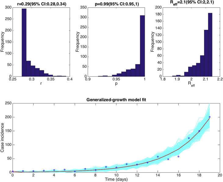
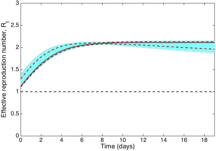
We assumed an exponential distribution for the generation interval of influenza with a mean of 4 days and variance of 16. Using the early growth phase in the number of new case notifications during the first 20 epidemic days, we estimated the deceleration of growth parameter at 0.99 (95% CI: 0.95, 1.0), an epidemic growth profile with uncertainty bounds that includes exponential growth dynamics (i.e., p = 1) (Fig. 19). Based on the generalized-growth method, we estimated the effective reproduction number at 2.1 (95% CI: 2.0, 2.1) (Fig. 20).

Fig. 19.

Top panels display the empirical distributions of the growth rate $r$, the deceleration of growth parameter $p$ and the effective reproduction number $R_{eff}$ based on fitting the GGM to the first 20 days of the 1918 influenza pandemic in San Francisco. We assumed an exponential distribution for the generation interval of influenza with a mean of 4 days and variance of 16. The bottom panel shows the fit of the GGM to the first 20 days of the 1918 influenza pandemic in San Francisco. Circles correspond to the data while the solid red line corresponds to the best fit obtained using the generalized-growth model (GGM). The blue lines correspond to the uncertainty around the model fit. We estimated the deceleration of growth parameter at 0.95 (95%CI: 0.95, 1.0), an epidemic growth profile with uncertainty bounds that includes exponential growth dynamics (i.e., p = 1) during the early growth trajectory of the pandemic in Madrid.

Fig. 20.

The effective reproduction number estimated during the first 20 days of the 1918 influenza pandemic in San Francisco using the GGM. We assumed an exponential distribution for the generation interval of influenza with a mean of 4 days and variance of 16. The solid red line corresponds to mean effective reproduction number while the dashed lines correspond to the 95% confidence bounds around the mean. The blue lines correspond to the uncertainty.

15. Discussion and future work

In this article we have described and illustrated a relatively simple computational approach to quantify parameter uncertainty, evaluate parameter identifiability, assess model performance, and generate forecasts with quantified uncertainty. In the process we have employed simple phenomenological and mechanistic models to characterize epidemic patterns as well as estimate key transmission parameters such as the basic reproduction number $R_0$ and the effective reproduction number $R_t$. This uncertainty quantification approach is computationally intensive and relies solely on case incidence series from an unfolding outbreak and allows considerations of different error structures in the case series data (e.g., Poisson vs. negative binomial).

In future research we will build on this framework to address issues related to model uncertainty (Lloyd Chowellet al, 2009). In particular, researchers often focus on a given model and data to characterize the state of the system, but less on how different sets of assumptions influence parameter estimates, their uncertainty and impact on forecasts. Instead of relying on a single model, the information provided by multiple contending models can be integrated into ensemble models (e.g., model weighting schemes (Burnham & Anderson, 2002)), analogous to weather prediction systems (Raftery et al., 2005).

Appendix A. Supplementary data

The following is the supplementary data related to this article:

References

- Anderson R.M., May R.M. Directly transmitted infections diseases: Control by vaccination. Science. 1982;215(4536):1053–1060. doi: 10.1126/science.7063839. [DOI] [PubMed] [Google Scholar]
- Anderson R.M., May R.M. Oxford University Press; , Oxford: 1991. Infectious diseases of humans. [Google Scholar]
- Arriola L., Hyman J.M. Sensitivity analysis for uncertainty quantification in mathematical models. In: Chowell G., editor. Mathematical and statistical estimation approaches in epidemiology. Springer Netherlands; 2009. pp. 195–247. [Google Scholar]
- Bailey N.T.J. Hafner; , New York: 1975. The mathematical theory of infectious disease and its applications. [Google Scholar]
- Banks H.T. An inverse problem statistical methodology summary. In: Chowell G., editor. Mathematical and statistical estimation approaches in epidemiology. 2009. pp. 249–302. [Google Scholar]
- Banks H.T., Hu S., Thompson W.C. CRC Press; 2014. Modeling and inverse problems in the presence of uncertainty. [Google Scholar]
- Brauer F. Some simple epidemic models. Mathematical Biosciences and Engineering. 2006;3(1):1–15. doi: 10.3934/mbe.2006.3.1. [DOI] [PubMed] [Google Scholar]
- Brauer F., Nohel J.A. Courier Corporation; 2012. The qualitative theory of ordinary differential equations: anintroduction. [Google Scholar]
- Burnham K.P., Anderson D.R. Springer-Verlag; , New York: 2002. Model selection and multimodel inference: A practical information-theoretic approach. [Google Scholar]
- Capaldi A. Parameter estimation and uncertainty quantification for an epidemic model. Mathematical Biosciences and Engineering. 2012;9(3):553–576. doi: 10.3934/mbe.2012.9.553. [DOI] [PubMed] [Google Scholar]
- Chowell G., Brauer F. The basic reproduction number of infectious diseases: Computation and estimation using compartmental epidemic models. In: Chowell G., editor. Mathematical and statistical estimation approaches in epidemiology. Springer; 2009. [Google Scholar]
- Chowell G. Transmission dynamics of the great influenza pandemic of 1918 in Geneva, Switzerland: Assessing the effects of hypothetical interventions. Journal of Theoretical Biology. 2006;241(2):193–204. doi: 10.1016/j.jtbi.2005.11.026. [DOI] [PubMed] [Google Scholar]
- Chowell G. Modelling the transmission dynamics of acute haemorrhagic conjunctivitis: Application to the 2003 outbreak in Mexico. Statistics in Medicine. 2006;25(11):1840–1857. doi: 10.1002/sim.2352. [DOI] [PubMed] [Google Scholar]
- Chowell G. The Western Africa ebola virus disease epidemic exhibits both global exponential and local polynomial growth rates. PLoS Currents. 2015:7. doi: 10.1371/currents.outbreaks.8b55f4bad99ac5c5db3663e916803261. [DOI] [PMC free article] [PubMed] [Google Scholar]
- Chowell G. Mathematical models to characterize early epidemic growth: A review. Physics of Life Reviews. 2016;(16):30064–30071. doi: 10.1016/j.plrev.2016.07.005. pii: S1571-0645. [DOI] [PMC free article] [PubMed] [Google Scholar]
- Chowell G. Using phenomenological models to characterize transmissibility and forecast patterns and final burden of Zika epidemics. PLOS Currents Outbreaks. 2016 doi: 10.1371/currents.outbreaks.f14b2217c902f453d9320a43a35b9583. pii:ecurrents.outbreaks.f14b2217c902f453d9320a43a35b9583. [DOI] [PMC free article] [PubMed] [Google Scholar]
- Chowell G. Characterizing the reproduction number of epidemics with early sub-exponential growth dynamics. Journal of The Royal Society Interface. 2016;13(123) doi: 10.1098/rsif.2016.0659. p. pii: 20160659. [DOI] [PMC free article] [PubMed] [Google Scholar]
- Chowell G. Perspectives on model forecasts of the 2014-2015 ebola epidemic in West Africa: Lessons and the way forward. BMC Medicine. 2017;15(1):42. doi: 10.1186/s12916-017-0811-y. [DOI] [PMC free article] [PubMed] [Google Scholar]
- Chowell G., Nishiura H., Bettencourt L.M. Comparative estimation of the reproduction number for pandemic influenza from daily case notification data. Journal of The Royal Society Interface. 2007;4(12):155–166. doi: 10.1098/rsif.2006.0161. [DOI] [PMC free article] [PubMed] [Google Scholar]
- Chowell G., Viboud C. Is it growing exponentially fast? – Impact of assuming exponential growth for characterizing and forecasting epidemics with initial near-exponential growth dynamics. Infectious Disease Modelling. 2016;1(1):71–78. doi: 10.1016/j.idm.2016.07.004. [DOI] [PMC free article] [PubMed] [Google Scholar]
- Cobelli C., Romanin-Jacur G. Controllability, observability and structural identifiability of multi input and multi output biological compartmental systems. IEEE Transactions on Biomedical Engineering. 1976;23(2):93–100. doi: 10.1109/tbme.1976.324568. [DOI] [PubMed] [Google Scholar]
- Diekmann O., Heesterbeek J.A., Metz J.A. On the definition and the computation of the basic reproduction ratio R0 in models for infectious diseases in heterogeneous populations. Journal of Mathematical Biology. 1990;28(4):365–382. doi: 10.1007/BF00178324. [DOI] [PubMed] [Google Scholar]
- Dinh L. Estimating the subcritical transmissibility of the Zika outbreak in the State of Florida, USA, 2016. Theoretical Biology and Medical Modelling. 2016;13(1):20. doi: 10.1186/s12976-016-0046-1. [DOI] [PMC free article] [PubMed] [Google Scholar]
- van den Driessche P., Watmough J. Reproduction numbers and sub-threshold endemic equilibria for compartmental models of disease transmission. Mathematical Biosciences. 2002;180:29–48. doi: 10.1016/s0025-5564(02)00108-6. [DOI] [PubMed] [Google Scholar]
- Efron B., Tibshirani R.J. CRC Press; 1994. An introduction to the bootstrap. [Google Scholar]
- Fauci A.S., Morens D.M. Zika virus in the americas–yet another arbovirus threat. New England Journal of Medicine. 2016;374(7):601–604. doi: 10.1056/NEJMp1600297. [DOI] [PubMed] [Google Scholar]
- Hsieh Y.H., Cheng Y.S. Real-time forecast of multiphase outbreak. Emerging Infectious Diseases. 2006;12(1):122–127. doi: 10.3201/eid1201.050396. [DOI] [PMC free article] [PubMed] [Google Scholar]
- Jacquez J.A. Michigan: Michigan Thompson-Shore Inc; 1996. Compartmental analysis in biology and medicine. [Google Scholar]
- Kuhn M., Johnson K. Vol. 26. Springer; New York: 2013. (Applied predictive modeling). [Google Scholar]
- Lee J., Chowell G., Jung E. A dynamic compartmental model for the Middle East respiratory syndrome outbreak in the Republic of Korea: A retrospective analysis on control interventions and superspreading events. Journal of Theoretical Biology. 2016;408:118–126. doi: 10.1016/j.jtbi.2016.08.009. [DOI] [PMC free article] [PubMed] [Google Scholar]
- Lloyd A.L. Sensitivity of Model-based epidemiological parameter estimation to model assumptions. In: Chowell G., editor. Mathematical and statistical estimation approaches in epidemiology. Springer; 2009. pp. 123–141. [Google Scholar]
- Ma J. Estimating initial epidemic growth rates. Bulletin of Mathematical Biology. 2014;76(1):245–260. doi: 10.1007/s11538-013-9918-2. [DOI] [PubMed] [Google Scholar]
- Nishiura H., Chowell G. The effective reproduction number as a prelude to statistical estimation of time-dependent epidemic trends. In: Chowell G., editor. Mathematical and statistical estimation approaches in epidemiology. Springer; The Netherlands: 2009. pp. 103–121. [Google Scholar]
- Pell B. Using phenomenological models for forecasting the 2015 Ebola challenge. Epidemics. 2016 doi: 10.1016/j.epidem.2016.11.002. [DOI] [PubMed] [Google Scholar]
- Pillonetto G., Sparacino G., Cobelli C. Numerical non-identifiability regions of the minimal model of glucose kinetics: Superiority of bayesian estimation. Mathematical Biosciences. 2003;184(1):53–67. doi: 10.1016/s0025-5564(03)00044-0. [DOI] [PubMed] [Google Scholar]
- Raftery A.E. Using Bayesian model averaging to calibrate forecast ensembles. Monthly Weather Review. 2005;133(5):1155–1174. [Google Scholar]
- Raue A. Structural and practical identifiability analysis of partially observed dynamical models by exploiting the profile likelihood. Bioinformatics. 2009;25(15):1923–1929. doi: 10.1093/bioinformatics/btp358. [DOI] [PubMed] [Google Scholar]
- Richards F.J. A flexible growth function for empirical use. Journal of Experimental Botany. 1959;10(2):290–301. [Google Scholar]
- Sattenspiel L. Princeton University Press; 2009. The geographic spread of infectious diseases: Models and applications. [Google Scholar]
- Smirnova A., Chowell G. A primer on stable parameter estimation and forecasting in epidemiology by a problem-oriented regularized least squares algorithm. Infectious Disease Modeling. May 2017;2(2):268–275. doi: 10.1016/j.idm.2017.05.004. [DOI] [PMC free article] [PubMed] [Google Scholar]
- Strogatz Steven H. Westview press; 2014. Nonlinear dynamics and chaos: with applications to physics, biology, chemistry, and engineering. [Google Scholar]
- Turner M.E.J. A theory of growth. Mathematical Biosciences. 1976;29(3–4):367–373. [Google Scholar]
- Viboud C., Simonsen L., Chowell G. A generalized-growth model to characterize the early ascending phase of infectious disease outbreaks. Epidemics. 2016;15:27–37. doi: 10.1016/j.epidem.2016.01.002. [DOI] [PMC free article] [PubMed] [Google Scholar]
- Wallinga J., Lipsitch M. How generation intervals shape the relationship between growth rates and reproductive numbers. Proceedings of the Royal Society B: Biological Sciences. 2007;274(1609):599–604. doi: 10.1098/rspb.2006.3754. [DOI] [PMC free article] [PubMed] [Google Scholar]
- Wang X.S., Wu J., Yang Y. Richards model revisited: Validation by and application to infection dynamics. Journal of Theoretical Biology. 2012;313:12–19. doi: 10.1016/j.jtbi.2012.07.024. [DOI] [PubMed] [Google Scholar]
Associated Data
This section collects any data citations, data availability statements, or supplementary materials included in this article.