Gene Density and Chromosome Territory Shape

Abstract

Despite decades of study of chromosome territories (CT) in the interphase nucleus of mammalian cells, our understanding of the global shape and 3-D organization of the individual CT remains very limited. Past microscopic analysis of CT suggested that, while many of the CT appear to be very regular ellipsoid-like shapes, there were also those with more irregular shapes. We have undertaken a comprehensive analysis to determine the degree of shape regularity of different CT. To be representative of the whole human genome, 12 different CT (~41% of the genome) were selected that ranged from the largest (CT 1) to the smallest (CT 21) in size and from the highest (CT 19) to lowest (CT Y) in gene density. Using both visual inspection and algorithms that measure the degree of shape ellipticity and regularity, we demonstrate a strong inverse correlation between the degree of regular CT shape and gene density for those CT that are most gene rich (19, 17, 11) and gene poor (18, 13, Y). CT more intermediate in gene density, showed a strong negative correlation with shape regularity but not with ellipticity. An even more striking correlation between gene density and CT shape was determined for the nucleolar associated NOR-CT. Correspondingly striking differences in shape between the X active and inactive CT implied that, aside from gene density, the overall global level of gene transcription on individual CT is also an important determinant of chromosome territory shape.

Introduction

Chromosomes in the interphase nucleus do not appear as the X-shaped entities characteristic of mitosis (Cremer and Cremer 2001; Cremer and Cremer 2010; Stack et al. 1977; Zorn et al. 1979). Instead, they occur as three dimensional structures termed chromosome territories (CT) (Cremer and Cremer 2010; Cremer et al. 2006; Cremer et al. 2000; Lichter et al. 1988; Manuelidis 1985; Meaburn and Misteli 2007; Schardin et al. 1985; Tajbakhsh et al. 2000; Visser and Aten 1999). While the details of CT associations and their degree of non-randomness is still under investigation, studies to date support a high degree of non-random but probabilistic arrangements between various CT that show cell type and tissue specificity in human cells (Boyle et al. 2001; Marella et al. 2009; Zeitz et al. 2009). Moreover, the spatial arrangement of CT inside the nucleus are dependent on their size (Sun et al. 2000) and gene density (Kreth et al. 2004).

Despite this progress, our knowledge of how DNA is arranged three-dimensionally into individual territories and their overall morphology as CT is still in its infancy. Initially, CT were reported to acquire a nearly spherical shape (Edelmann et al. 2001), with gene rich CT19 occupying a less compacted territory than the gene poor CT18 (Croft et al. 1999). Differences in the shapes of active X (Xa) and inactive X (Xi) chromosomes (Eils et al. 1996) were found in which Xi had a smoother and rounder surface while Xa was larger with a more irregular surface (Eils et al. 1996).

The shapes of CT potentially depend on the relative content of the heterochromatin and euchromatin. Open chromatin fibers originate from gene rich domains or ridges (Gilbert et al. 2004). These ridges are less condensed and more irregularly shaped than the gene poor anti-ridges (Goetze et al. 2007). Live cell studies of CT revealed complex CT shapes. These findings suggested that different chromosomes may have different shapes and provided a basis for our current study.

To establish a better understanding of chromosome shapes, we have undertaken a study of 12 different chromosomes in WI-38 and MRC5 normal human fibroblast cells. Based on visual inspection and computer algorithms, we quantitatively measured the shape and regularity of the chromosomes. We determined that the overall shape and regularity of CT at the extreme ends of gene density (most gene rich and most gene poor) correlate with gene density. Very gene-rich chromosomes were highly irregular in shape and very gene-poor chromosomes were more regular ellipsoid-like. A significant correlation between gene density and the degree of shape regularity was also found for chromosomes which are of intermediate gene densities. Moreover, despite having the same gene densities, striking differences in the shape regularity were demonstrated for the two homologs of CT X (Xa vs Xi). These findings are discussed in terms of the role of gene density and activity in chromosome territory shape.

Results

Despite decades of study of chromosome territories (CT) in the interphase nucleus of mammalian cells, (Bickmore 2013; Cremer and Cremer 2010; Lanctot et al. 2007; Meaburn and Misteli 2007; Misteli 2004; Parada et al. 2004a; Parada et al. 2004b) our understanding of the global shape and 3-D organization of the individual CT remains very limited. With this in mind, we have undertaken a comprehensive analysis to determine the shape regularity of different CT in WI38 normal diploid human lung fibroblast cells. To be representative of the overall human genome, 12 different CT (~ 41% of the genome) were selected ranging from the largest (CT 1) to the smallest (CT 21) in size and from the highest (CT 19) to lowest (CT Y) in gene density.

Shape Categorization Based on Visual Classification

While it is commonly assumed that chromosome territories generally have an ellipsoid-like shape (Khalil et al. 2007), our initial observations of this large subset of CT suggested wide variations in shape. Some chromosomes appeared “compact” with a regular ellipsoid-like shape, while others displayed more of an “open” structure – sometimes with several protrusions or “looping out” of chromatin from the main body of the CT and/or highly convoluted borders. Moreover, the degree of shape regularity appeared to be characteristic of each chromosome. In chromosome 17, for example, a large proportion of the observed CT had highly irregular shapes with multiple projections extending in various directions (Fig 1). In contrast, chromosome Y territories were predominantly of a regular ellipsoid-like shape with only a very minor proportion of highly irregularly shaped CT (Fig 2–3). Detailed visual inspection led us to divide each CT into three shape categories: 1) regular- a compact regular ellipsoid-like shape; 2) slightly irregular- an expanded more open ellipsoid-like shape often containing a single protrusion and/or limited levels of undulation along the CT borders; 3) moderately to highly Irregular- even more open and loose structures with major undulations and/or projections along the CT borders. The 12 human chromosomes classified into the above categories (100 – 150 CT images were analyzed for each chromosome number) included: CT 19,17,11 (3 most gene rich), Y,13,18 (3 most gene poor), 22,1,12,X (intermediate gene densities) and the nucleolar associated chromosomes (22,15,21,13). The classification was performed without knowledge of the chromosome under inspection. Representative 2-D projection images illustrating the three shape categories for each CT are presented along with their corresponding border outlines in Figure 2. It is important to emphasize that all the chromosomes from gene rich to gene poor had significant levels of shapes ranging from highly regular to highly irregular. What was distinctive for each chromosome was the distribution of these three shape categories in the population of each CT.

Fig. 1. Irregularity in chromosome territory 17 shape.

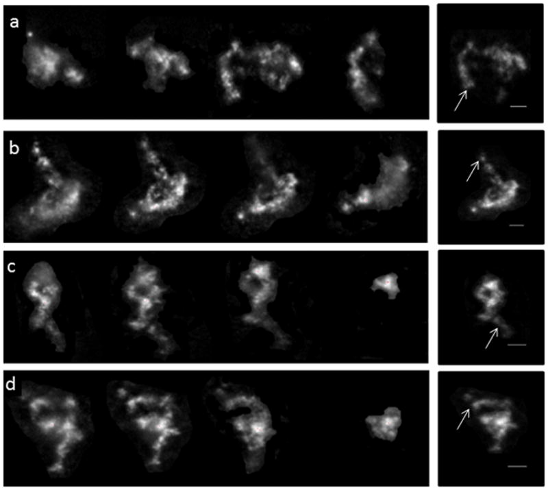
Individual optical sections transversing 4 different CT 17 (one homolog) are shown (a–d). 2-D projection images for the combined sections of each CT are depicted on the extreme right panels. Arrows point to “looping out and projections”. Scale bar represents 2 μm

Fig. 2. Projection images and contours of chromosome territories.

The chromosome territory (CT) projection images were divided into 3 categories based on the degree of shape irregularity (1- regular, 2-slightly irregular, 3- moderately to highly irregular). (a) gene rich CT: 19 (a–c), 17 (g–i) and 11 (m–o). The shape classifications were made based on the contours for the same 2-D projection images after applying the ImageJ threshold plug-in (CT 19, d–f; CT 17, j–l; CT 11, p–r); (b) gene poor CT: 18 (a–c), 13 (g–i) and Y (m–o). The shape classifications were made based on the contours for the same 2-D projection images after applying the ImageJ threshold plug-in (CT 18 d–f; CT 13, j–l; CT Y, p–r); (c) (a) 2-D projection image of the active (Xa) and the inactive (Xi) CT X; (b) contours for the same image after applying the ImageJ threshold plug-in; 3-D surface rendering images showing irregular shaped CT 22 (red) and regular shaped CT 13 (green) in the same cell (c), and irregular shaped CT 19 (red) and regular shaped CT 18 (green) in the same cell (d). This suggests that differences observed in the degree of CT irregularity are not an artifact of the FISH procedure. Scale bar represents 2 μm; grid depicts 50 μm² in Fig c(c, d)

Fig. 3. Shape distributions of chromosome territories.

(a) % distribution of 3 gene rich CT (19, 17, and 11) and 3 gene poor (18, 13, and Y) in the 3 shape categories; (b) linear regression analysis demonstrates a negative correlation (r² = 0.70) between the % distribution of regular CT shapes and gene density for (a); (c) linear regression demonstrates a very weak negative correlation (r² = 0. 27) between the % distribution of slightly irregular CT shapes and gene density for (a); (d) linear regression demonstrates a positive correlation (r² = 0.73) between the % distribution of moderately to highly irregular CT shapes and gene density for (a); (e) % distribution of intermediate gene density CT (22,1,12, and X) in the 3 shape categories; (f) linear regression indicates a negative correlation (r² = 0.70) between the % distribution of regular CT shapes and gene densities for (e); (g) no linear correlation is found (r² = 0.001) between the % distribution of slightly irregular CT shapes and gene density for (e); (h) linear regression demonstrates a weak correlation (r² = 0.43) between the % distribution of moderately to highly irregular CT shapes and gene density for (e); (i) % distribution of the nucleolar associated CT (22, 15, 21, and 13) in the 3 shape categories; (j) linear regression analysis depicts a negative correlation (r² = 0.78) between gene density and the % distribution of regular nucleolar CT shapes; (k) linear regression demonstrates a moderate negative correlation (r² = 0.63) between gene density and % slightly irregular; (l) linear regression shows a positive correlation (r² = 0.74) of moderate to highly irregular nucleolar CT shapes and gene density; (m) The % distributions of the two X CT demonstrate huge differences in shape regularity between Xa and Xi; n = 100–150 CT images for each distribution study

Figure 3a shows the % chromosome distribution into the three shape categories for the three most gene rich and most gene poor chromosomes. The gene poor CT had higher percentages (38–56%) in the “regular” category while the gene rich CT were higher (38%–70%) in the “moderately to highly irregular” category. A linear regression analysis performed on the gene rich/gene poor CT distributions revealed a negative correlation (r² = 0.70) between the % distribution in the regular category and chromosome gene densities (Fig 3b) and a positive correlation (r²= 0.73) in the moderately to highly irregular category (Fig 3d). No correlation was found between the % slightly irregular and gene density (r² = 0.27, Fig 3c). These findings indicate that the very gene rich CT (9.2 – 22.5 genes/mbp) have more open and irregular shapes while the very gene poor chromosomes (1.1 – 3.3 genes/mbp) had larger proportions of more regularly shaped CT. Similar results were found for the NOR-containing nucleolar associated chromosomes (Fig 3i–l), which also have a wide range of gene densities (2.7 to 8.2 genes/mbp). While the chromosomes with intermediate gene density (5.2 to 8.2 genes/mbp) (Fig 3e), showed a negative correlation (r² = 0.70) between the % distribution in the regular shape category and gene densities (Fig 3f), there was only a very weak positive correlation (r²= 0.43) in the moderately to highly Irregular category (Fig 3h), and no correlation in the slightly irregular category (Fig 3g).

A striking difference in shape distributions was found between the two homologs of chromosome X. The inactive Xi homolog had a more regular, compact shape (Fig 2c(a, b)) with nearly 65% in the regular category (Fig 3m) compared to < 25% (Fig 3m) for the much more irregularly shaped Xa (Fig 2c(a, b)). To further rule out the possibility that the differences in the CT shapes were due to variations in labeling from one experiment to the next, dual labeling FISH experiments were performed in which one relatively gene rich and one gene poor chromosome were labeled at the same time in the same cells. Two different pairs of chromosomes were analyzed (CT 13–22 and CT 18–19) with virtually identical shape distribution patterns as those where only single CT were labeled (data not shown). Representative images showing these double labeled CT are shown in Figure 2C.

To determine whether there is a difference in the shape regularity between 2 homologous chromosomes in the same nucleus, we visually classified the 2 homologs of the same CT into the 3 categories (category 1 – regular, category 2 – slightly irregular, and category 3 – moderately to highly irregular). The CT investigated were gene rich CT 17, CT 11, intermediate gene density CT 12, CT X, and gene poor CT 18. CTs 17, 11, 12, and 18 had the highest % of homologs in the same category (72%–88%) compared to 26% for the CT X homologs (supplementary Fig S1). These findings demonstrate a significant level of similarity in the shape regularity of CT homologs in individual cells other than CT X.

Linear regression analyses performed on the three shape categories and the gene densities of the entire subset of chromosomes revealed a weak negative correlation between the % regular CT and gene density (r² = 0.52; supplementary Fig S2a). While no correlation was observed for the slightly irregular category (r² = 0.19, supplementary Fig S2b), a weak positive correlation was obtained for the moderately to highly irregular category (r² = 0.51; supplementary Fig S2c). No correlation (r² = 0.002–0.14) was found between chromosome size (mbp) and the % of CT in the regular, slightly irregular, and the moderately to highly irregular categories (Supplementary Fig S3 (a–c). Thus chromosome size has no apparent effect on shape regularity.

Determining Chromosome Territory Shape by Computational Analysis

Our visual observations and categorizations (Fig 1–3) prompted us to develop computational approaches to measure the degree of both the ellipticity (e) and the regularity (r) of the CT shapes (see Materials and Methods). For ellipticity, e = 1.0 only if the shape is a perfect ellipsoid. Shapes that deviate from an ellipsoid have progressively lower values (Zunic and Zunic 2013). To quantitate the variation in the regular shape of different CT, we developed an algorithm that evaluates the overall degree of shape regularity rather than conformity to a given type of shape such as an ellipsoid (Berg et al. 2008). We term this the “regularity or r algorithm” and it determines the ratio of the total area of the CT (a) and the convex hull area (cha) or a/cha (see Materials and Methods, Fig 6h). Analogous to the e-algorithm, the ratio of a/cha or r for an absolutely regular shape, is 1.0 and increasingly lower values correspond to progressive increases in shape irregularity (Fig 6h).

Fig. 6. Chromosome territory shape regularity.

An r value of 1.0 denotes a perfectly regular structure, e.g. an oval, while decreasing values indicate increasing levels of irregularity in the CT shape. (a) 3 most gene rich (19, 17, 11) and the 3 most gene poor (18,13,Y) CT; (c) CT with intermediate gene densities (22, 1, 12, 4); (e) nucleolar associated CT 22, 15, 21, and 13; (g) Xa vs Xi; regression analysis revealed a linear correlation (r² = 0.79) between r and the gene densities of the most gene rich and poor CT (b) as well as with CT (d) having intermediate gene densities (r² = 0.87); (f) depicts a very strong linear correlation (r² = 0.98) of r and gene density for the nucleolar associated CT; (h) schematic diagram showing a hypothetical chromosome territory (blue solid line) and the convex hull of that shape (red dotted line); error bars represent SEM

A series of simulated shapes were run through both these algorithms before applying them to the actual chromosome images (Figure 4a–f). The simulated structures ranged from a regular ellipsoid and a triangle to considerably irregular ellipsoid-like shapes with protrusions coming off of the main body. The latter mimic the range of different shapes which were directly observed for the different CT. Running both algorithms on the simulated images verified their expected properties. The perfect ellipsoid had an ellipticity (e) value of 1 and a perfect score in terms of regularity (Fig 4a). The extended and irregular ellipsoid-like structure of Figure 4c had a significant ellipsoid score (0.83) but a lower one for regularity (0.73). The perfect triangle, on the other hand, scored a low value for e (0.70), but a perfect regularity score. The irregular ellipsoids shapes in Figure 4d, and 4e were exactly the same except for two thread-like projections or “looping-outs” in 4e. Addition of the “looping-outs” drastically lowered both the e- and r-values (Fig 4e). Finally, a highly convoluted and extended shape had low e- and r- values (Fig 4f).

Fig. 4. Computer simulations of shapes and 3-D surface rendering of chromosome territories.

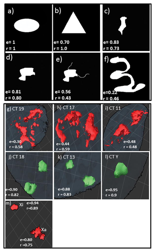
Simulated images (a–f) were constructed in imageJ and run through the computer algorithms to determine the ellipticity (e), and shape regularity (r) obtained over a range of simulated chromosomes from highly regular- denoted by an ellipsoid, and a triangle (a,b) - to highly irregular denoted by both an irregular shape and “looping out” (e, f); (g–m) representative 3-D surface rendering images and the e, and r values for the 3 most gene rich CT 19(g), 17(h), and 11(i); the 3 most gene poor CT 18 (j), 13 (k), and Y (l); and CT Xa vs Xi (m). Grid represents 50 μm²

Representative 3-D surface rendering images of the 3 most gene rich and 3 most gene poor CT and chromosome X along with their e- and r-values are depicted in Figures 4g–m. A good correlation is seen between the algorithm scores and the shapes displayed in the microscopic images. More extensive determinations of e- and r-values performed on actual CT images, led to the conclusion that values of e ≥ 0.77, and r ≥ 0.75, denote a considerably degree of ellipsoid-like and regular shapes, respectively. With this as a basis we applied these two algorithms on our entire CT image sets.

Ellipticity of Chromosome Territories

A high degree of ellipticity was measured for the most gene poor chromosomes ranging from 0.83 for CT Y to 0.75 for CT 13 (Fig 5a). The 2 most gene rich chromosomes, CT 19 and CT 17, had e values that deviated significantly from regular ellipsoid shapes (0.62 and 0.66 respectively), while CT 11, which has the lowest gene density of the top three had a value of 0.77 (Fig 5a). 7 of the 9 possible combinations comparing the ellipticity for the gene-rich and gene-poor CT showed significant differences (p< 0.05). No significant differences were observed in the ellipticity values between the gene rich chromosome 11, and gene poor chromosomes − 13, and 18. Linear regression analysis demonstrated a strong negative correlation (r² = 0.87) between gene density and the degree of regular ellipsoid shape (Fig 5b).

Fig. 5. Chromosome territory shape ellipticity.

An e value of 1.0 denotes a perfectly regular ellipsoid while decreasing values indicate increasing levels of irregularity in the CT shape. (a) 3 most gene rich (19, 17, 11) and the 3 most gene poor (18,13,Y) CT; (c) CT with intermediate gene densities (22, 1, 12, X); (e) nucleolar associated CT 22, 15, 21, and 13; (g) Xa vs Xi; (b) linear regression analysis revealed a strong linear correlation (r² = 0.87) between the ellipticity and the gene densities of the most gene rich and poor CT but a weak correlation (r² = 0.56) with CT having intermediate gene densities (d); (f) depicts a strong linear correlation (r² = 0.85) with the nucleolar associated CT; error bars represent SEM

The ellipticity test was also applied to CT with intermediate gene densities (CT 22, 1, 12 and X; Fig 5c). Statistically significant differences (p<0.05) were found in 5 out of 6 combinations of ellipticity values among these 4 chromosomes except for combinations involving CT 1, and CT 12. Linear regression analysis showed only a weak correlation between e-values and gene density (r² = 0.56, Fig 5d). In contrast, analysis of the ellipticity versus gene density for the four nucleolar associated CT (22, 15, 21, 13, Fig 5e) revealed a strong negative correlation (r² = 0.85, Fig 5f). Consistent with our visual observations and measurements (Fig 1–4), CT Xi had the highest value for ellipticity (0.90), while CT Xa had a much lower level (0.73, Fig 5g). Moreover, the overall linear regression analysis with all 12 chromosomes together had an r² value of 0.35, depicting at best a very weak correlation between e-values and gene density (Fig S2d). No correlation was found between the chromosome size (mbp) and ellipticity of the CT (r² = 0.08, supplementary Fig S3 (d)).

Shape Regularity of Chromosome Territories

Applying the regularity r algorithm to the image sets revealed that the most gene poor chromosome Y had an r value closest to 1.0 (0.84) followed by the gene poor chromosomes 18 and 13 at 0.77 and 0.79, respectively (Fig 6a). The r-value for the most gene rich CT 19 was 0.71, followed by CT 17 (0.73) and CT 11 (0.75). 8 of the 9 possible combinations comparing the regularity for the gene-rich and gene-poor CT showed significant differences (p< 0.05). Linear regression analysis further demonstrated a good correlation (r²= 0.79) between the r-values and the gene densities for the 3 most gene rich and 3 most gene poor CT (Fig 6b).

For CT with intermediate gene densities, r ranged from 0.70 for CT 22 to 0.81 for CT X (Fig 6c). Highly significant differences in r-values were found among these 4 chromosomes except for combinations involving CT 1 and CT 12. The linear regression analysis showed a strong negative correlation between the r-values and their respective gene densities (r² = 0.87, Fig 6d). Moreover, analysis of the r-values versus gene density for the four nucleolar associated CT (Fig 6e) revealed a nearly perfect negative correlation (r² = 0.98, Fig 6f). Intriguingly, Xa and Xi showed striking differences in regularity (0.76 vs 0.86; p<10⁻⁹, Fig 6g). This is significant since Xa and Xi have the same gene densities but they differ highly in gene activity. Xi also showed greater levels of ellipticity than Xa (Fig 4 and 5). While the regression analysis of all the 12 chromosomes together revealed an r² value of 0.50, suggesting a weak correlation between r values and gene density (Fig S2e), chromosome size did not seem to have any effect on CT shape regularity (r² = 0.01, supplementary Fig S3e).

Shape Regularity during the Cell Cycle

Next we investigated whether the overall degree of shape regularity is altered between the G1 and S phases of the cell cycle in WI38 cells. Five different CT were analyzed including the gene rich CT 17, gene poor CT 18, CT 1 and 12 with intermediate gene densities and CT Xa/Xi. Visual classification of shape regularity revealed only minor differences in the distribution profiles between the G1 and S phases for CT 17, 18 and X, but much greater differences for CT 1, and 12 where there was a large increase in the percentage of irregular structures in S phase compared to G1 (Fig 7a and S4a–d). Computational analysis using the regularity algorithm confirmed these findings (Fig 7b). Statistically significant differences were measured (p<0.05) in the r-values for CT 1 (0.78 in G1, 0.74 in S), and 12 (0.76 in G1, 0.72 in S) but not for CT, 17, 18 or X (Fig 7b).

Fig. 7. Chromosome territory shape during G1 and S phase.

Visual classification (a) and computational analysis (b) was performed on CT 17, 1, 12, Xa/Xi, and 18 in cells which were in either G1 or S phase of the cell cycle. There were no significant differences in the shape regularity in the 2 cell cycle stages for CT 17, Xa/Xi, and 18 but striking differences for CT 1, and 12 (p<0.05), as indicated by the asterisks; error bars represent SEM

Discussion

Spatial positioning has emerged as a fundamental principle governing nuclear processes (Berezney 2002; Berezney et al. 2005; Bickmore 2013; Kumaran et al. 2008; Lanctot et al. 2007; Malyavantham et al. 2008; Malyavantham et al. 2010; Stein et al. 2003; Zaidi et al. 2007). While it is now well accepted that chromosomes occupy discrete bodies in the interphase cell nucleus termed chromosome territories (CT) (Cremer and Cremer 2010; Cremer et al. 2006; Cremer et al. 2000; Lichter et al. 1988; Manuelidis 1985; Meaburn and Misteli 2007; Schardin et al. 1985; Tajbakhsh et al. 2000; Visser and Aten 1999), we are just beginning to unravel the degree to which the CT are organized and the resulting effects on gene regulation (Bickmore 2013; Cremer and Cremer 2010; Lanctot et al. 2007; Meaburn and Misteli 2007; Misteli 2004; Parada et al. 2004a; Parada et al. 2004b). For example, our understanding of the overall shape of CT is very limited. Earlier studies suggested non-spherical shapes for human CT 7 and X (Eils et al. 1995; Eils et al. 1996) and ellipsoid-like morphology for mouse CT 1, 11, 12, 15, 19 (Khalil et al. 2007). Moreover, the gene rich CT 19 was reported to occupy a less compacted territory and have a more irregular shape than the gene poor CT 18 (Croft et al. 1999). Similarly, the gene active CT Xa was found to have a more irregular and extended shape than its gene inactive CT Xi homolog (Bischoff et al. 1993; Eils et al. 1996; Walker et al. 1991). Differences in CT shapes across the population, and a relative maintenance of these shapes for up to four hours in the cell cycle were further suggested from live cell analyses (Edelmann et al. 2001; Muller et al. 2010). Thus studies to date have been limited to a handful of chromosomes and no detailed investigations have been performed of CT shapes, their regularities, and the factors affecting their shapes.

In this investigation we have undertaken a systematic analysis of CT shape by both direct visualization and application of computational programs which precisely quantitate the degree of ellipsoidal shape and regularity. A subset of 12 chromosomes were selected which are representative of the wide range of chromosome size and gene densities in the human genome. This included: a) the 3 most gene rich and most gene poor chromosomes; b) chromosomes with average gene densities; c) nucleolar associated chromosomes; and d) chromosome X_active (Xa) and X_inactive (Xi). Visual examination of hundreds of images for each CT revealed regular ellipsoid-like shapes for the most gene-poor chromosomes, while the most gene rich ones had very irregular shapes. We confirmed these observations by application of newly developed algorithms that quantitate the degree of ellipticity (e) and overall regularity (r) of the CT shapes. The degree of ellipsoidal or shape regularity varied from chromosome to chromosome. All the chromosomes from gene rich to gene poor had significant levels of shapes ranging from highly regular to highly irregular. What was distinctive for each chromosome was the distribution of these three shape categories in the population of each CT. Live cell studies (Edelmann et al. 2001; Muller et al. 2010) performed on CT shapes in the past have also reported differences in the CT shapes within the population as opposed to the general belief that CT are just spherical or ellipsoid in shape. Consistently, we found that Chromosome 17, for example, demonstrated both a high degree of irregularity within the main body of the CT as well as projections extending up to microns in length away from the main body (Fig 1). CT 19 also had highly irregular shapes but with lesser levels of projections and the gene poor chromosomes Y, 13 and 18 were highly enriched in regular ellipsoid-like shapes (Fig 2). Similar linear relationships between shape regularity and gene density for the most gene rich and poor CT were determined by visual scoring of images as well as by measurements of ellipticity and shape regularity (Fig 3,5,6). This was also the case for the nucleolar associated CT (13, 15, 21, and 22) and to a lesser extent the CT with moderate gene densities (CT X, 12, 1 and 22).

Several chromosomes in this study have a similar mbp size but large differences in gene densities. CT 19 and Y are at the extreme ends of gene density but are virtually identical in mbp size. Other CT pairs of similar mbp size but vastly different in gene densities are: CT 17/18, CT 11/13, and CT 21/22. The striking dissimilarity between the shape regularity in the above mentioned CT pairs with equivalent sizes supports the view that gene density and not chromosome size, plays a major role in the global architecture of CT. Moreover, linear regressive analysis revealed no correlation between chromosome size and shape regularity (Fig S3).

We further analyzed the shape regularity between the two homologs of the same CT in the same cell. A similar regularity was found in a large majority of cells (72–88%) for CT ranging from gene-rich to gene-poor (CT 17, 11, 12, and 18) but not for CT X (26%, Fig S1). Thus chromosome homologs in individual cells are largely similar in their degree of shape regularity even though each CT as a total population has a characteristic range of regularity.

Aside from gene density a role of transcription in chromosome shape is suggested by the striking differences in shape regularity between Xa and Xi. If this is the case, it would be expected that inhibition of transcription would result in a corresponding change in the shape of Xa toward the more condensed Xi shape. While an earlier study demonstrated this for CT19 (Croft et al. 1999), the study of Muller et al (2010) did not observe this alteration for CT11 in living cells. In another recent study transcriptional inhibition resulted in the compaction in the overall structure of Xa to the level of Xi and led these investigators to propose that transcription and gene activity do affect CT shapes ((Naughton et al. 2010). Our measurements of CT X confirmed previous findings (Eils et al. 1995; Eils et al. 1996) of striking differences in the shapes of Xi (regular and ellipsoid-like) and Xa (irregular and less ellipsoidal) and further demonstrated a remarkable similarity in the morphology of the transcriptionally inactive Xi and CT Y. CT Y is the most gene poor chromosome and displays very limited transcriptional activities (Flicek et al. 2014; Quintana-Murci and Fellous 2001). From these findings we conclude that gene activity influences CTX shape regularity and possibly that of CTY. Generalization to the other chromosomes, however, will require further investigation.

Differences in CT shapes might also be related to corresponding differences in chromatin folding. Gene rich CT like 19, 17, and 22 (the fourth most gene dense) are abundant in open chromatin fibers and along each chromosome there is a strong correlation between the presence of open chromatin and regions of high gene density (Gilbert et al. 2004). In contrast, gene poor CT like 18, 13, and Y have much lower levels of open chromatin fibers which correlate with regions containing increased levels of closed chromatin and low gene density (Gilbert et al. 2004). Transcriptome mapping has further identified chromosomal regions (typically ranging from 5 to 25 mbp) of increased gene expression (ridges) and regions of low gene expression (anti-ridges) (Caron et al. 2001). Moreover, ridges are generally of high gene density, while anti-ridges have low gene densities (Caron et al. 2001; Gierman et al. 2007). More detailed analysis at the mbp level has revealed that the chromatin present in ridges is much less compact and more irregular in shape than the chromatin in anti-ridges (Gierman et al. 2007; Goetze et al. 2007). These previous findings of local chromosomal shape alterations at the mbp level are remarkably similar to what we have found for the global shapes of CT.

Although CT 11 is the third most gene rich chromosome (9.2 genes/mbp), it was overall more regular in shape than CT 22 (8.2 genes/mbp). CT 11, also has an unusually low content of open chromatin fibers for a gene rich chromosome as compared to other gene rich CT 19, and 17, and the intermediate gene dense CT 22 (Gilbert et al. 2004). It is even lower than some of the moderate gene density CT including 12 (Gilbert et al. 2004). Thus the degree and arrangement of open versus close chromatin regions in CT may also be an important determinate of CT shape along with gene density and activity. A role of steric hindrance in CT shape is also likely considering the crowded microenvironment of the cell nucleus (Muller et al. 2010).

Numerous investigations demonstrate that long-range chromosomal interactions (both intrachromosomal and interchromosomal) occur in a transcriptionally dependent manner to regulate gene expression (Clowney et al. 2012; Osborne et al. 2004; Osborne et al. 2007; Spilianakis et al. 2005). These chromosomal interactions provides a potential mechanism for distally located genes to cluster in close proximity at “transcription factories” for gene function or silencing (Clowney et al. 2012; Malyavantham et al. 2008; Malyavantham et al. 2010; Mitchell and Fraser 2008; Osborne et al. 2004; Osborne et al. 2007; Williams et al. 2010). The CT shape irregularities observed in this investigation may provide the structural basis to enhance both intrachromosomal and interchromosomal interactions. Large scale projections or “looping out” of certain gene-rich domains have been reported in correlation with gene activation (Gilbert et al. 2004; Volpi et al. 2000; Williams et al. 2002). The finger-like projections of up to several microns that we have observed enriched in the gene rich chromosomes may correspond to these regions of active gene expression. In this scenario the projections would provide the means for genes to increase the distance they can transverse for productive gene expression. “Looping out” protrusions were also observed in the gene poor chromosomes (Fig 2), but at a much lower frequent than in the gene rich chromosomes (Fig 1). CT with intermediate gene densities also displayed occasional projections (Fig 2).

Positioning of CT within the nucleus is likely to also have an impact on their shape. The nucleolar associated CT show high levels of association with the nucleoli which inevitably effects the overall shapes of these chromosomes as do the associations of CT with the nuclear periphery where the majority of the condensed heterochromatin is found. The peripherally located CT also have more interactions with the lamin proteins (Guelen et al. 2008). A role of nuclear matrix proteins in maintaining the overall territorial organization of chromosomes has also been reported (Berezney et al. 2005; Croft et al. 1999; Ma et al. 1999). We propose that the final shape of CT are a result of the interactions of several factors such as open chromatin levels, gene density, gene activity and transcription, positioning in the cell nucleus, associations with other nuclear proteins, and steric constraints as proposed by (Muller et al. 2010). Moreover, our findings of statistically significant differences for at least some of the CT in the degree of overall shape regularity between the G1 and S phases are consistent with a dynamic nature of global CT shapes that can be altered in concert with corresponding alterations in the overall transcriptional program during the cell cycle.

Materials and Methods

Cell Culture

ATCC human lung fibroblast cell lines WI38 and MRC5 were grown in advanced Dulbecco’s Modified Eagle Medium supplemented with 10% serum and penicillin-streptomycin at 37°C, 5% CO₂.

DNA FISH (Fluorescence In-situ hybridization) and Immunofluorescence

Cells were treated with trypsin at ~80% confluency, placed on coverslips and grown overnight. Fixation was carried out using 4% paraformaldehyde for 10 min, followed by treatment with PBS-glycine for 20 min. Cells involved in cell cycle studies were pulsed with 20 μM Edu for 30 min before fixation. Cells were permeabilized using 0.5% Triton X-100 (25 min), and incubated in 20% glycerol/1X PBS for 1 h. Four rounds of freeze thaws were carried out in liquid nitrogen followed by treatment with 0.1N HCl for 5 min. The coverslips were stored in 50% formamide/2XSSC at 4°C until denaturation was carried out at 75°C for 9 min in 70% formamide/2 X SSC followed by ice cold 50% formamide/2 X SSC for 5 min. Probe paints for chromosomes 1(DEAC fluorophore), 11 (DEAC fluorophore), 12 (DEAC fluorophore), 13 (Texas red fluorophore), 15 (Texas red fluorophore), 17 (DEAC fluorophore), 18 (DEAC fluorophore), 19 (Texas red fluorophore), 21 (Texas red fluorphore), 22 (DEAC fluorophore), X (DEAC fluorophore), and Y (Texas res fluorophore) were obtained from Chrombios GMBH, Nussdorf, Germany. The probes were denatured at 75°C for 10 min. The coverslips were then inverted on the probe solution and sealed with rubber cement. Hybridization was carried out at 37°C for 48 h in a moist chamber. Three post hybridization washes for 45 min each at 37°C contained in order: 50% formamide / 2XSSC/0.05% Tween-20; 2 X SSC/0.05% Tween 20; and 1 X SSC. All the chromosomes were labeled in female WI38 cells except for chromosome Y, which was labeled in male MRC5 cells. For cells involved in cell cycle studies, S phase cells were selected based on EdU incorporation (Cavanagh et al. 2011). EdU was detected using the Click-iT EdU detection kit (Life Technologies, Chicago, IL) following the manufacturer’s protocol with minor variations. The G1 population was distinguished from G2 by singlet/doublet analysis (Fritz et al. 2013) using BAC probes that labeled 6 regions throughout the length of the chromosome. The G2 population was not analyzed in this study.

Microscopy

Images were captured with an Olympus 100X,1.4 NA objective on an Olympus BX 51 (Olympus America Inc., Center Valley, PA) microscope equipped with a Sensicam QE digital CCD camera (Cooke Corporation, Romulus, MI), a motorized z-axis controller (Prior), Slidebook 4.0 (Intelligent Imaging Innovations, Denver, CO) and Image-Pro plus 4.1 (Media Cybernetics, Inc., Bethesda, MD) softwares. Optical sections (0.5 μm) were collected, deblurred using the “NoNeighbor algorithm” within Slidebook 4.0, and exported as 16-bit tiff intensity files for further analysis.

Identification of Xa and Xi territories

The images obtained after labeling CT X were merged with the DAPI image of the respective nucleus. The colocalization of one of the copies of CT X with the highly intense DAPI region in the nucleus (Barr Body) resulted in the identification of the Xinactive ((Teller et al. 2011); Fig S5). The Barr body was easily recognizable in ~85% of the image sets. Image sets in which this distinction could not be made were not used for analysis.

Visual Classification of Shape Regularity

Images of different chromosomes types were mixed and labels were removed in order to classify their shape regularity without knowing their identity. Background reduction was performed using the background subtraction plug in on Image J (National Institutes of Health, Bethesda Maryland). The chromosome boundary (contour) was then obtained manually, using Image J’s threshold plug in. The chromosomes were then visually classified into three broad categories- 1) regular, 2) slightly irregular, 3) moderately to highly irregular. All optical sections for each image set were inspected as a basis for classification. 100–150 CT images were analyzed for each chromosome.

Computer Analysis and Statistics

Algorithms were developed to measure the level of shape regularity for each image set that was previously evaluated by visual inspection. In the first algorithm, termed the ellipticity or e-algorithm, the closeness of a shape to an ellipsoid was measured. This algorithm (Zunic and Zunic 2013), is a significant improvement over previously developed algorithms. In this approach, it is assumed that all ellipses are of the same shape regardless their axis-ratios. Basically, three steps are used to accomplish the measurement – First, the CT shape is normalized.

Definition 1

For a given shape S, S is said to be normalized if:

1. The area of S is 1;

2. The centroid of S coincides with the origin;

3. The orientation O(S) of S is 0.

The orientation (Rosin 2005; Zunic et al. 2006) of a shape means the line that minimizes the integral of the squared distance of shape’s points to this line. For example, in an ellipsoid, the orientation is its long axis. The orientation is 0 means the long axis is parallel to X axis.

Then we compute ellipticity measure ε(S) from geometric moments to be the direct measurement of closeness to ellipsoid.

Definition 2

Geometric moments m_p,q(S) of a planar shape S is defined as

$$m_{p,q}(\mathrm{S})={\iint }_S{x}^p{y}^q\mathit{dxdy}$$

Definition 3

The ellipticity measure ε(S) is defined as

$$\epsilon (S)=\frac{1}{2}\ast \frac{1}{a{(S)}^2\ast m_{2,0}(S)+b{(S)}^2\ast m_{0,2}(S)}$$

Where $a(S)=\sqrt{2{\pi }^{2}L(S)-\pi \ast \sqrt{4{\pi }^{2}L{(S)}^2-1}},b(S)=\sqrt{2{\pi }^{2}L(S)+\pi \ast \sqrt{4{\pi }^{2}L{(S)}^2-1}}$ and L(S) = m_2,0(S) + m_0,2(S)

It’s proved in (Zunic and Zunic 2013) that ε(S) = 1 ⇔ S ia an ellipsoid. And the range of ε(S) is (0,1].

Starting from calculating several geometric moments, we can obtain the ellipticity measure ε of a chromosome territory. The more ε close to 1, the more the territory is close to an ellipsoid.

In the second algorithm, termed the regularity or r-algorithm, the overall degree of shape regularity was measured. In this algorithm, the area ratio of each chromosome territory over its convex hull (a/cha) was determined. The convex hull CH(S) of a set S is the smallest convex set that contains S. To be more precise, it is the intersection of all convex sets that contains (S) (Berg et al. 2008). If a chromosome is regular, the ratio of its area over its convex hull area will be close to 1. An Increase in irregularity will result in a corresponding decrease of the a/cha ratio. Figure 6h illustrates the convex hull of a hypothetical chromosome territory. The chromosome boundary is depicted with a solid blue line, while the convex hull of that territory is shown as a dashed red line. To calculate the ratio of area/convex hull area (a/cha), convex hulls of chromosome territories were first obtained using the (function: bwconvhull) in MATLAB and then area of chromosome territories and area of convex hulls were separately obtained using the (function bwarea).

To optimize the accuracy of the measurements for both algorithms (e- and r-values) each CT copy was subjected to the computer programs individually. After background subtraction using Image J, the upper and the lower limits of the image threshold were determined manually using the threshold plugin in Image J. These upper and lower threshold limits were then plugged into the algorithms running in MATLAB. The algorithms analyzed all the 3-D sections of a given CT image, and generated values for each section of the image. The e- or r- values for CT in each image set was then expressed as the average of all the in focus sections. The output file for each individual CT was then manually compiled into a composite MS excel file to allow for further analysis. To determine whether or not differences in measurements were statistically significant, student’s t-tests were carried out on the results and all comparisons with p-values below 0.05 were determined to be significant.

Supplementary Material

supplement

Supplementary Fig. S1 Visual Distribution of CT homologs in the 3 categories. Visual classification in the 3 shape categories was performed on CT 17, 12, X, and 18. Scoring was then performed to find out what % of homologs fell into the – a) same category (1, 2, or 3), b) one homolog belonging to category 1, and the other to category 2 (category 1_2), c) one homolog belonging to category 2, and the other to category 3 (category 2_3), d) one homolog belonging to category 1, and the other to category 3 (category 1_3)

Supplementary Fig. S2 Linear regression analysis for the entire subset of 12 CT. (a) A weak negative correlation (r² = 0.52) was obtained between % regular CT and gene densities of the entire subset, (b) the linear regression analysis between % slightly irregular CT and gene densities revealed no correlation (r² = 0.19). (c) Correlation analysis performed between % moderately to highly irregular categories and gene densities for the entire CT subset depicted a weak positive correlation (r² = 0.51). (d) Linear regression analysis between the gene density and the e-values for the entire subset of CT shows a very weak correlation (r² = 0.35). (e) Regression analysis between gene density and r-values of the entire CT subset demonstrates a weak negative correlation (r² = 0.55).

Supplementary Fig. S3 Size has no effect on shape regularity/ellipticity. Linear regression analysis was performed between chromosome sizes (in mbp) and the CT distribution in regular (a), slightly irregular (b), moderately to highly irregular (c) and between chromosome sizes and the e-values (d) or r-values (e). No correlation was observed in any of these cases (r² = 0.002 – 0.14).

Supplementary Fig. S4. Representative images showing differences in CT shapes in G₁ and S phase. Significant differences in the CT 1, and 12 shape regularity are observed in G₁ and S phase. Representative images elucidating these differences are shown in this figure. (a) CT 1 in G₁ phase, (b) CT 1 in S phase, (c) CT 12 in G₁, and (d) CT 12 in S phase.

Supplementary Fig. S5. Identification of the X_inactive (Xi) CT. (a) DAPI labeling of the nucleus. Arrow marks the highly intense DAPI labeling; (b) CT X label in that nucleus, arrow pointing at the compact X CT; (c) Merged image – arrow pointing at the overlap of the intense DAPI with the boundry of the “compact” CT X, identified as Xi.

References

- Berezney R. Regulating the mammalian genome: the role of nuclear architecture. Advances in enzyme regulation. 2002;42:39–52. doi: 10.1016/s0065-2571(01)00041-3. [DOI] [PubMed] [Google Scholar]
- Berezney R, Malyavantham KS, Pliss A, Bhattacharya S, Acharya R. Spatio-temporal dynamics of genomic organization and function in the mammalian cell nucleus. Advances in enzyme regulation. 2005;45:17–26. doi: 10.1016/j.advenzreg.2005.02.013. [DOI] [PubMed] [Google Scholar]
- Berg Md, Cheong O, Kreveld Mv, Overmars M. Computational Geometry: Algorithms and Applications. 3. Springer; 2008. [Google Scholar]
- Bickmore WA. The spatial organization of the human genome. Annual review of genomics and human genetics. 2013;14:67–84. doi: 10.1146/annurev-genom-091212-153515. [DOI] [PubMed] [Google Scholar]
- Bischoff A, Albers J, Kharboush I, Stelzer E, Cremer T, Cremer C. Differences of size and shape of active and inactive X-chromosome domains in human amniotic fluid cell nuclei. Microscopy research and technique. 1993;25:68–77. doi: 10.1002/jemt.1070250110. [DOI] [PubMed] [Google Scholar]
- Boyle S, Gilchrist S, Bridger JM, Mahy NL, Ellis JA, Bickmore WA. The spatial organization of human chromosomes within the nuclei of normal and emerin-mutant cells. Human molecular genetics. 2001;10:211–219. doi: 10.1093/hmg/10.3.211. [DOI] [PubMed] [Google Scholar]
- Caron H, et al. The human transcriptome map: clustering of highly expressed genes in chromosomal domains. Science. 2001;291:1289–1292. doi: 10.1126/science.1056794. [DOI] [PubMed] [Google Scholar]
- Cavanagh BL, Walker T, Norazit A, Meedeniya AC. Thymidine analogues for tracking DNA synthesis. Molecules. 2011;16:7980–7993. doi: 10.3390/molecules16097980. [DOI] [PMC free article] [PubMed] [Google Scholar]
- Clowney EJ, et al. Nuclear aggregation of olfactory receptor genes governs their monogenic expression. Cell. 2012;151:724–737. doi: 10.1016/j.cell.2012.09.043. [DOI] [PMC free article] [PubMed] [Google Scholar]
- Cremer T, Cremer C. Chromosome territories, nuclear architecture and gene regulation in mammalian cells. Nature reviews Genetics. 2001;2:292–301. doi: 10.1038/35066075. [DOI] [PubMed] [Google Scholar]
- Cremer T, Cremer M. Chromosome territories. Cold Spring Harbor perspectives in biology. 2010;2:a003889. doi: 10.1101/cshperspect.a003889. [DOI] [PMC free article] [PubMed] [Google Scholar]
- Cremer T, Cremer M, Dietzel S, Muller S, Solovei I, Fakan S. Chromosome territories--a functional nuclear landscape. Current opinion in cell biology. 2006;18:307–316. doi: 10.1016/j.ceb.2006.04.007. [DOI] [PubMed] [Google Scholar]
- Cremer T, et al. Chromosome territories, interchromatin domain compartment, and nuclear matrix: an integrated view of the functional nuclear architecture. Critical reviews in eukaryotic gene expression. 2000;10:179–212. [PubMed] [Google Scholar]
- Croft JA, Bridger JM, Boyle S, Perry P, Teague P, Bickmore WA. Differences in the localization and morphology of chromosomes in the human nucleus. The Journal of cell biology. 1999;145:1119–1131. doi: 10.1083/jcb.145.6.1119. [DOI] [PMC free article] [PubMed] [Google Scholar]
- Edelmann P, Bornfleth H, Zink D, Cremer T, Cremer C. Morphology and dynamics of chromosome territories in living cells. Biochimica et biophysica acta. 2001;1551:M29–39. doi: 10.1016/s0304-419x(01)00023-3. [DOI] [PubMed] [Google Scholar]
- Eils R, et al. Application of confocal laser microscopy and three-dimensional Voronoi diagrams for volume and surface estimates of interphase chromosomes. Journal of microscopy. 1995;177:150–161. doi: 10.1111/j.1365-2818.1995.tb03545.x. [DOI] [PubMed] [Google Scholar]
- Eils R, et al. Three-dimensional reconstruction of painted human interphase chromosomes: active and inactive X chromosome territories have similar volumes but differ in shape and surface structure. The Journal of cell biology. 1996;135:1427–1440. doi: 10.1083/jcb.135.6.1427. [DOI] [PMC free article] [PubMed] [Google Scholar]
- Flicek P, et al. Ensembl 2014. Nucleic Acids Res. 2014;42:D749–D755. doi: 10.1093/Nar/Gkt1196. [DOI] [PMC free article] [PubMed] [Google Scholar]
- Fritz A, Sinha S, Marella N, Berezney R. Alterations in replication timing of cancer-related genes in malignant human breast cancer cells. Journal of cellular biochemistry. 2013;114:1074–1083. doi: 10.1002/jcb.24447. [DOI] [PMC free article] [PubMed] [Google Scholar]
- Gierman HJ, et al. Domain-wide regulation of gene expression in the human genome. Genome research. 2007;17:1286–1295. doi: 10.1101/gr.6276007. [DOI] [PMC free article] [PubMed] [Google Scholar]
- Gilbert N, Boyle S, Fiegler H, Woodfine K, Carter NP, Bickmore WA. Chromatin architecture of the human genome: gene-rich domains are enriched in open chromatin fibers. Cell. 2004;118:555–566. doi: 10.1016/j.cell.2004.08.011. [DOI] [PubMed] [Google Scholar]
- Goetze S, et al. The three-dimensional structure of human interphase chromosomes is related to the transcriptome map. Molecular and cellular biology. 2007;27:4475–4487. doi: 10.1128/MCB.00208-07. [DOI] [PMC free article] [PubMed] [Google Scholar]
- Guelen L, et al. Domain organization of human chromosomes revealed by mapping of nuclear lamina interactions. Nature. 2008;453:948–951. doi: 10.1038/nature06947. [DOI] [PubMed] [Google Scholar]
- Khalil A, Grant JL, Caddle LB, Atzema E, Mills KD, Arneodo A. Chromosome territories have a highly nonspherical morphology and nonrandom positioning. Chromosome research : an international journal on the molecular, supramolecular and evolutionary aspects of chromosome biology. 2007;15:899–916. doi: 10.1007/s10577-007-1172-8. [DOI] [PubMed] [Google Scholar]
- Kreth G, Finsterle J, von Hase J, Cremer M, Cremer C. Radial arrangement of chromosome territories in human cell nuclei: a computer model approach based on gene density indicates a probabilistic global positioning code. Biophysical journal. 2004;86:2803–2812. doi: 10.1016/S0006-3495(04)74333-7. [DOI] [PMC free article] [PubMed] [Google Scholar]
- Kumaran RI, Thakar R, Spector DL. Chromatin dynamics and gene positioning. Cell. 2008;132:929–934. doi: 10.1016/j.cell.2008.03.004. [DOI] [PMC free article] [PubMed] [Google Scholar]
- Lanctot C, Cheutin T, Cremer M, Cavalli G, Cremer T. Dynamic genome architecture in the nuclear space: regulation of gene expression in three dimensions. Nature reviews Genetics. 2007;8:104–115. doi: 10.1038/nrg2041. [DOI] [PubMed] [Google Scholar]
- Lichter P, Cremer T, Borden J, Manuelidis L, Ward DC. Delineation of individual human chromosomes in metaphase and interphase cells by in situ suppression hybridization using recombinant DNA libraries. Human genetics. 1988;80:224–234. doi: 10.1007/BF01790090. [DOI] [PubMed] [Google Scholar]
- Ma H, Siegel AJ, Berezney R. Association of chromosome territories with the nuclear matrix. Disruption of human chromosome territories correlates with the release of a subset of nuclear matrix proteins. The Journal of cell biology. 1999;146:531–542. doi: 10.1083/jcb.146.3.531. [DOI] [PMC free article] [PubMed] [Google Scholar]
- Malyavantham KS, Bhattacharya S, Alonso WD, Acharya R, Berezney R. Spatio-temporal dynamics of replication and transcription sites in the mammalian cell nucleus. Chromosoma. 2008;117:553–567. doi: 10.1007/s00412-008-0172-6. [DOI] [PMC free article] [PubMed] [Google Scholar]
- Malyavantham KS, Bhattacharya S, Berezney R. The architecture of functional neighborhoods within the mammalian cell nucleus. Advances in enzyme regulation. 2010;50:126–134. doi: 10.1016/j.advenzreg.2009.10.003. [DOI] [PMC free article] [PubMed] [Google Scholar]
- Manuelidis L. Individual interphase chromosome domains revealed by in situ hybridization. Human genetics. 1985;71:288–293. doi: 10.1007/BF00388453. [DOI] [PubMed] [Google Scholar]
- Marella NV, Bhattacharya S, Mukherjee L, Xu J, Berezney R. Cell type specific chromosome territory organization in the interphase nucleus of normal and cancer cells. Journal of cellular physiology. 2009;221:130–138. doi: 10.1002/jcp.21836. [DOI] [PubMed] [Google Scholar]
- Meaburn KJ, Misteli T. Cell biology: chromosome territories. Nature. 2007;445:379–781. doi: 10.1038/445379a. [DOI] [PubMed] [Google Scholar]
- Misteli T. Spatial positioning; a new dimension in genome function. Cell. 2004;119:153–156. doi: 10.1016/j.cell.2004.09.035. [DOI] [PubMed] [Google Scholar]
- Mitchell JA, Fraser P. Transcription factories are nuclear subcompartments that remain in the absence of transcription. Genes & development. 2008;22:20–25. doi: 10.1101/gad.454008. [DOI] [PMC free article] [PubMed] [Google Scholar]
- Muller I, Boyle S, Singer RH, Bickmore WA, Chubb JR. Stable morphology, but dynamic internal reorganisation, of interphase human chromosomes in living cells. PloS one. 2010;5:e11560. doi: 10.1371/journal.pone.0011560. [DOI] [PMC free article] [PubMed] [Google Scholar]
- Naughton C, Sproul D, Hamilton C, Gilbert N. Analysis of active and inactive X chromosome architecture reveals the independent organization of 30 nm and large-scale chromatin structures. Molecular cell. 2010;40:397–409. doi: 10.1016/j.molcel.2010.10.013. [DOI] [PMC free article] [PubMed] [Google Scholar]
- Osborne CS, et al. Active genes dynamically colocalize to shared sites of ongoing transcription. Nature genetics. 2004;36:1065–1071. doi: 10.1038/ng1423. [DOI] [PubMed] [Google Scholar]
- Osborne CS, et al. Myc dynamically and preferentially relocates to a transcription factory occupied by Igh. PLoS biology. 2007;5:e192. doi: 10.1371/journal.pbio.0050192. [DOI] [PMC free article] [PubMed] [Google Scholar]
- Parada LA, McQueen PG, Misteli T. Tissue-specific spatial organization of genomes. Genome biology. 2004a;5:R44. doi: 10.1186/gb-2004-5-7-r44. [DOI] [PMC free article] [PubMed] [Google Scholar]
- Parada LA, Sotiriou S, Misteli T. Spatial genome organization. Experimental cell research. 2004b;296:64–70. doi: 10.1016/j.yexcr.2004.03.013. [DOI] [PubMed] [Google Scholar]
- Quintana-Murci L, Fellous M. The Human Y Chromosome: The Biological Role of a “Functional Wasteland”. Journal of biomedicine & biotechnology. 2001;1:18–24. doi: 10.1155/S1110724301000080. [DOI] [PMC free article] [PubMed] [Google Scholar]
- Rosin PL. Computing global shape measures. In: Chen CH, Wang PSP, editors. Handbook of Pattern Recognition and Computer Vision. World Scientific; 2005. pp. 177–196. [Google Scholar]
- Schardin M, Cremer T, Hager HD, Lang M. Specific staining of human chromosomes in Chinese hamster x man hybrid cell lines demonstrates interphase chromosome territories. Human genetics. 1985;71:281–287. doi: 10.1007/BF00388452. [DOI] [PubMed] [Google Scholar]
- Spilianakis CG, Lalioti MD, Town T, Lee GR, Flavell RA. Interchromosomal associations between alternatively expressed loci. Nature. 2005;435:637–645. doi: 10.1038/nature03574. [DOI] [PubMed] [Google Scholar]
- Stack SM, Brown DB, Dewey WC. Visualization of interphase chromosomes. Journal of cell science. 1977;26:281–299. doi: 10.1242/jcs.26.1.281. [DOI] [PubMed] [Google Scholar]
- Stein GS, et al. Functional architecture of the nucleus: organizing the regulatory machinery for gene expression, replication and repair. Trends in cell biology. 2003;13:584–592. doi: 10.1016/j.tcb.2003.09.009. [DOI] [PubMed] [Google Scholar]
- Sun HB, Shen J, Yokota H. Size-dependent positioning of human chromosomes in interphase nuclei. Biophysical journal. 2000;79:184–190. doi: 10.1016/S0006-3495(00)76282-5. [DOI] [PMC free article] [PubMed] [Google Scholar]
- Tajbakhsh J, Luz H, Bornfleth H, Lampel S, Cremer C, Lichter P. Spatial distribution of GC- and AT-rich DNA sequences within human chromosome territories. Experimental cell research. 2000;255:229–237. doi: 10.1006/excr.1999.4780. [DOI] [PubMed] [Google Scholar]
- Teller K, et al. A top-down analysis of Xa- and Xi-territories reveals differences of higher order structure at >/= 20 Mb genomic length scales. Nucleus. 2011;2:465–477. doi: 10.4161/nucl.2.5.17862. doi: http://dx.doi.org/10.4161/nucl.2.5.17862. [DOI] [PubMed] [Google Scholar]
- Visser AE, Aten JA. Chromosomes as well as chromosomal subdomains constitute distinct units in interphase nuclei. Journal of cell science. 1999;112(Pt 19):3353–3360. doi: 10.1242/jcs.112.19.3353. [DOI] [PubMed] [Google Scholar]
- Volpi EV, et al. Large-scale chromatin organization of the major histocompatibility complex and other regions of human chromosome 6 and its response to interferon in interphase nuclei. Journal of cell science. 2000;113(Pt 9):1565–1576. doi: 10.1242/jcs.113.9.1565. [DOI] [PubMed] [Google Scholar]
- Walker CL, Cargile CB, Floy KM, Delannoy M, Migeon BR. The Barr body is a looped X chromosome formed by telomere association. Proceedings of the National Academy of Sciences of the United States of America. 1991;88:6191–6195. doi: 10.1073/pnas.88.14.6191. [DOI] [PMC free article] [PubMed] [Google Scholar]
- Williams A, Spilianakis CG, Flavell RA. Interchromosomal association and gene regulation in trans. Trends in genetics : TIG. 2010;26:188–197. doi: 10.1016/j.tig.2010.01.007. [DOI] [PMC free article] [PubMed] [Google Scholar]
- Williams RR, Broad S, Sheer D, Ragoussis J. Subchromosomal positioning of the epidermal differentiation complex (EDC) in keratinocyte and lymphoblast interphase nuclei. Experimental cell research. 2002;272:163–175. doi: 10.1006/excr.2001.5400. [DOI] [PubMed] [Google Scholar]
- Zaidi SK, et al. Nuclear microenvironments in biological control and cancer. Nature reviews Cancer. 2007;7:454–463. doi: 10.1038/nrc2149. [DOI] [PubMed] [Google Scholar]
- Zeitz MJ, Mukherjee L, Bhattacharya S, Xu J, Berezney R. A probabilistic model for the arrangement of a subset of human chromosome territories in WI38 human fibroblasts. Journal of cellular physiology. 2009;221:120–129. doi: 10.1002/jcp.21842. [DOI] [PubMed] [Google Scholar]
- Zorn C, Cremer C, Cremer T, Zimmer J. Unscheduled DNA synthesis after partial UV irradiation of the cell nucleus. Distribution in interphase and metaphase. Experimental cell research. 1979;124:111–119. doi: 10.1016/0014-4827(79)90261-1. [DOI] [PubMed] [Google Scholar]
- Zunic D, Zunic J. Shape Ellipticity Based on the First Hu Moment Invariant. Journal Information Processing Letters archive. 2013;113:807–810. [Google Scholar]
- Zunic J, Kopanja L, Fieldsend JE. Notes on shape orientation where the standard method does not work. Pattern Recognition. 2006;39:856–865. [Google Scholar]
Associated Data
This section collects any data citations, data availability statements, or supplementary materials included in this article.
Supplementary Materials