Unsupervised Myocardial Segmentation for Cardiac BOLD

Abstract

A fully automated 2D+time myocardial segmentation framework is proposed for Cardiac Magnetic Resonance (CMR) Blood-Oxygen-Level-Dependent (BOLD) datasets. Ischemia detection with CINE BOLD CMR relies on spatio-temporal patterns in myocardial intensity but these patterns also trouble supervised segmentation methods, the de-facto standard for myocardial segmentation in cine MRI. Segmentation errors severely undermine the accurate extraction of these patterns. In this paper we build a joint motion and appearance method that relies on dictionary learning to find a suitable subspace. Our method is based on variational pre-processing and spatial regularization using Markov Random Fields (MRF), to further improve performance. The superiority of the proposed segmentation technique is demonstrated on a dataset containing cardiac phase-resolved BOLD (CP-BOLD) MR and standard CINE MR image sequences acquired in baseline and ischemic condition across 10 canine subjects. Our unsupervised approach outperforms even supervised state-of-the-art segmentation techniques by at least 10% when using Dice to measure accuracy on BOLD data and performs at-par for standard CINE MR. Furthermore, a novel segmental analysis method attuned for BOLD time-series is utilized to demonstrate the effectiveness of the proposed method in preserving key BOLD patterns.

I. Introduction

Recent advances in Cardiac magnetic resonance (CMR) methods such as Cardiac Phase-resolved Blood-Oxygen-Level Dependent (CP-BOLD) MRI open up possibilities of direct and rapid assessment of ischemia [1]. In a single acquisition that can be seen together as a movie (i.e., similar to Standard CINE MRI acquisition), CP-BOLD provides both BOLD contrast and information of myocardial function [2]. Either at stress [3] or at rest (i.e., without any contraindicated provocative stress) [2], [4], BOLD signal intensity patterns are altered in a spatio-temporal manner. However, these patterns are subtle and changes occurring due to disease cannot be directly visualized [2]. In fact, identifying them requires significant post-processing, including myocardial segmentation and registration [5], prior to computer aided diagnosis via simple [3] or sophisticated pattern recognition methods [4]. This paper presents a segmentation method tailored to CP-BOLD MRI data, which is unsupervised and fully automated.

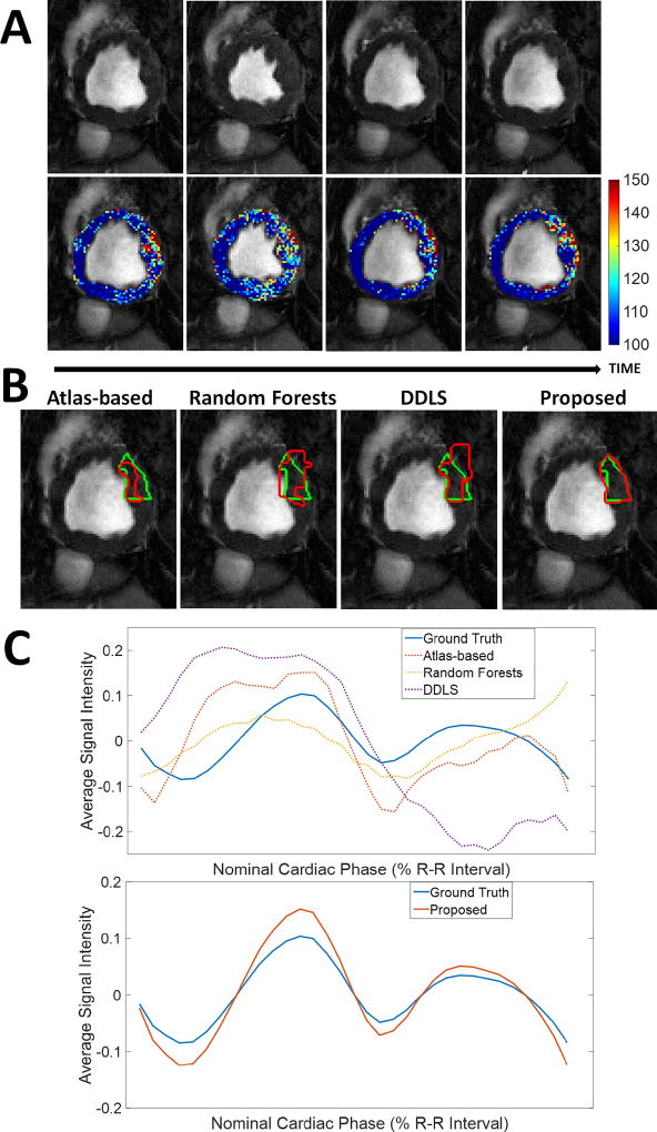
Currently, CP-BOLD myocardial segmentation requires tedious manual annotation. Despite advancements in this task in Standard CINE MRI (which is similar to CP-BOLD but with little or no BOLD contrast discussed at length at the related work section), most methods when used on CP-BOLD MR images for the same task, produce unsatisfactory results. Fig. 1B illustrates this by overlaying ground truth and algorithmic results for several state-of-the-art methods showing significant segmentation errors. These errors have deleterious effects on BOLD signals, as Fig. 1C shows. Instead of the expected behaviour across the cardiac cycle [2] which is seen when ground truth manual segmentations are used, significant deviations due to over- and under-segmentation are observed.

Fig. 1.

BOLD contrast challenges myocardial segmentation algorithms. A: Raw BOLD images from different cardiac phases of the same healthy subject) and color-coded myocardia overlaid on the raw images to demonstrate that subtle, imperceptible to the eye, intensity changes occur. B: Results of various algorithms (shown in red) for myocardial segmentation of the anterior region together with ground truth (green) manual delineations. Algorithms used: Atlas-based [6], Random Forests on Appearance and Texture features (a baseline) and a Dictionary Learning method (DDLS) [7]. C: Corresponding time series of the Anterior region from different methods compared to the one obtained based on ground truth segmentation. Overall errors in segmentation lead to deviations in the estimated time series, which will ultimately lead to low accuracy in ischemia detection. Our proposed method achieves high segmentation accuracy (last image in B); which leads to a better estimate of the time series (bottom part of C). [In typical CP-BOLD acquisition settings, with ECG-triggering, first and last points in the R-R interval correspond to diastole, whereas systole tends to appear around 30%.]

Although the BOLD contrast is visually subtle (as the top row of images in Fig. 1A shows) it can significantly affect segmentation performance. Locally these temporal variations influence registration performance [5], which results in under performance of Atlas-based techniques. Early on approaches tailored for BOLD MRI myocardial segmentation were semi-automated and relied on boundary tracking [8]. Later, fully automated but supervised methods [9] alleviated the need for interaction. However, there is an interest in methods that do not need vast amounts of training data and can easily adapt to data at hand and thus offer generalizability to unseen anatomical and pathological variation.

This paper presents a fully automated and unsupervised method for CP-BOLD MRI with the goal of faithfully preserving the key patterns necessary for diagnosis. The bottom of Fig. 1C illustrates the results of our method, which does not require any form of manual intervention e.g., landmark selection, ROI selection, spatio-temporal alignment to name a few. It builds upon a dictionary approach introduced in [9] using a joint appearance and motion model introduced in [10]¹. To increase robustness to the BOLD effect, we introduce a pre-processing step, that aims to “smooth out” temporal intensity variations. Subsequently, subject-specific dictionaries of patches of appearance and motion are built from a rudimentary definition of foreground (myocardium) and background (everything else). Projections on these discriminative dictionaries and spatial regularization with a Markov Random Field (MRF) obtains the final result. Extensive experiments show that, not only we obtain higher segmentation accuracy globally and locally around the myocardium, but also that this accuracy translates to better local preservation of BOLD patterns. Our work demonstrates that it is possible to train subject-specific dictionaries of background and foreground (myocardium) that jointly represent appearance and motion even when the training sets are drawn directly from the subject on the basis of a soft allocation of training patches. Together with atom pruning (which helps build an even more reliable collection of linear subspaces that span the data) and MRF overall leads to a robust automated and unsupervised algorithm (lacking external supervision) for myocardial segmentation.

The main contributions of this paper are:

• An unsupervised myocardial segmentation algorithm that uses dictionaries to jointly represent appearance and motion, trained on subject-specific data.

• The ability to extract meaningful data representations even when the data we learn from may not have the most precise annotation.

• Use of a variational spatio-temporal smoothing of the BOLD signal in a cardiac image sequence.

• Extensive segmentation performance analysis with both local and global measures.

The remainder of the paper is organized as follows: Section II offers a quick overview of approaches to myocardial segmentation for Standard CINE MRI. Section III presents the proposed method for myocardial segmentation in BOLD MRI. Experimental results are described in Section III-C. The final section offers discussion and conclusion.

II. Related Work

The automated myocardial segmentation for standard CINE MR is a well-studied problem [11], [12]. Most of the algorithms used for CINE MRI can be broadly classified into two categories based on whether the methodology is unsupervised or supervised. For the sake of brevity, we focus on examples most similar to our work.

Unsupervised methods

Although unsupervised segmentation techniques were employed early-on for myocardial segmentation of cardiac MR, almost all methods require minimal or advanced manual intervention [11]. Among the very few unsupervised techniques which are fully automated, the most similar to our proposed method are those that consider motion as a way to propagate an initial segmentation result to the whole cardiac cycle [13], [14], [15]. Grande et al. [16] integrates smoothness, image intensity and gradient related features in an optimal way under a MRF framework by Maximum Likelihood parameter estimation. Their deformable model estimates the walls based on the MRF along the short axis radial direction. A recent work [17] uses synchronized spectral networks for group-wise segmentation of cardiac images from multiple modalities. In our previous work [10], a fully automated joint motion and sparse representation based technique was proposed, where motion not only guides a rough estimate of the myocardium, but also leads to a smooth solution based on the movement of the myocardium.

Supervised Methods

Supervised approaches, on the other hand, have become the de-facto standard in recent years and in particular, Atlas-based supervised segmentation techniques have achieved significant success [11]. The myocardial segmentation masks available from other subject(s) are generally propagated to unseen data in Atlas-based techniques [18], [19] using non-rigid registration algorithms such as diffeomorphic demons (dDemons) [6], FFD-MI [20], and employ some fusion approaches to combine intermediate results (probabilistic label fusion or SVM) [19]. Segmentation techniques that do not use registration (to propagate contours), mainly rely on finding features that best represent the myocardium. Texture information is generally considered as an effective feature representation of the myocardium for standard CINE MR images [21]. Patch-based static discriminative dictionary learning technique (DDLS) [7] and Multi-scale Appearance Dictionary Learning technique [22] have achieved high accuracy and are considered as state-of-the-art mechanisms for supervised segmentation. Some methods utilize weak assumptions, such as spatial or intensity-based relations and anatomical assumptions, and include image-based techniques (threshold, dynamic programming, etc.) [23], pixel classification methods (clustering, Gaussian mixture model fitting, etc.) [24], [25], [16]. Strong prior methods include shape prior based deformable models [26], active shape and appearance models and Atlas-based methods, which focus on higher-level shape and intensity information and normally require a training dataset with manual segmentations [27]. Another idea is to exploit motion and temporal information within the acquired data. In [28] a graph cut algorithm is utilized by simultaneously exploiting motion and region cues. The method uses terminal nodes as moving objects and static background with the intention to extract a moving object surrounded by a static background. Spottiswoode et al. [29] used the encoded motion to project a manually-defined region of interest in the context of DENSE MRI. Both of these methods are semi-automated and need interaction to achieve high accuracy. Earlier, we proposed a supervised multi-scale discriminative dictionary learning (MSDDL) procedure [9]. However, unlike the proposed method, only appearance and texture features are considered for sparse representation in MSDDL. In general we can identify, that supervised methods require lots of data for training and a robust feature generation and matching framework. Finally briefly for completeness we mention deep learning methods that are fully supervised and aim to extract a hierarchy of image features at multiple scales (e.g. see [30], [31], [32], [33], [34], and a recent review [35]).

In this paper, we instead propose a fully unsupervised method that incorporates motion information in a dictionary learning framework.

III. Methods

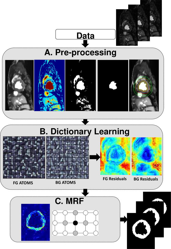
In the following we detail the proposed method for segmenting 2D(+time) Cardiac MRI data. The method does not rely on manual intervention and its only assumption is that motion patterns of the myocardium differ from those of surrounding tissues and organs. Our proposed method consists of three main blocks which are illustrated in Fig. 2 and described briefly below and in detail in the next sections.

Fig. 2.

Description of the proposed method. Block A aims to find a rough segmentation of the myocardium. In Block B two subject-specific dictionaries are trained on foreground and background on appearance and motion. In Block C a MRF-based segmentation algorithm on the residuals of the two dictionaries is utilized to have smooth boundaries.

The pre-processing block (Fig. 2A) aims to reduce BOLD effects by temporal smoothing using a Total Variation based method and to localize the myocardium to initialize the next step. The second block uses Dictionary Learning to obtain residuals (Fig. 2B). Subject-specific foreground and background dictionaries are trained from the two extracted regions from the entire cardiac sequence. These dictionaries are used to calculate the residuals of the cardiac image to be segmented. The final block introduces spatial regularization using Markov Random Field (MRF) approach, that is applied on the residuals of the two dictionaries to achieve the final segmentation of the myocardium (Fig. 2C). This block ensures the local smoothness of the extracted region.

A. Pre-processing

The overriding goal is to reduce the BOLD effect and obtain regions that patches can be drawn from for learning the dictionaries. This happens in few steps that we detail below and visually in Fig. 2A. First a Total Variation based filtering technique is used to smooth images to reduce the BOLD effect. Then, a process based on multi-level histogram thresholding is used to find the center of the Left Ventricle (LV) (on the mid-ventricular images we use here). We then segment the LV blood pool with region growing. Finally, aided by the distance transform we identify candidate foreground and background regions to sample from.

Total Variation based smoothing

The BOLD effect poses a significant problem to all state-of-the-art segmentation algorithms as demonstrated in [9] and discussed in the introduction. One way to create robustness is to learn intensity invariant features. However, [9] also demonstrated superior performance when using standard CINE MR. Inspired by this observation, we aim to identify a process that essentially converts the difficult CP BOLD MRI’s appearance into a more manageable standard CINE MR like appearance. Variational methods are used extensively in image denoising problems, most famous being the pioneering Rudin-Osher-Fatemi model [36]. Most of the video denoising methods derived from [36] actually work on a frame-by-frame basis. This approach is not suitable in our case since the BOLD effect is spatio-temporal across the cardiac cycle. In this work, we adopted the augmented Lagrangian method [37] developed in [38] to solve the BOLD inhomogeneity refinement problem in a space-time volume. We have employed the ℓ₁-norm Total Variation (ℓ₁-TV) using the augmented Lagrangian method introduced in [38] for solving both the problems together. The energy functional we have used for this particular minimization problem is:

$$\underset{f}{\text{minimize }}\frac{\mu }{2}{\Vert u-\upsilon \Vert }_1+{\Vert \nabla u\Vert }_2,$$

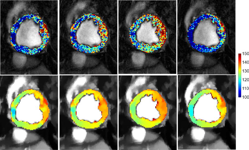
where υ is the input 2D+t image series and u is the processed image series. The main reason behind choosing ℓ₁-norm over ℓ₂-norm is the fact that appearances of different anatomies are piece-wise constant functions [39]. They also demonstrate quantized levels (i.e., a function can only take a given energy level without any other level existing between two anatomies), within a certain anatomy and sharp edges across anatomical boundaries. These boundaries and anatomies can be better preserved when using the ℓ₁-norm as shown in Fig. 4.

Fig. 4.

Influence of Total Variation based smoothing on different cardiac phases of a healthy subject. Four temporal phases of the same acquisition of a subject before (top) and after pre-processing (bottom), where myocardial intensities have been color-coded to aid visualization. Observe, how myocardial intensities appear smoother and within the same (and shorter) range across the cardiac cycle after TV-based smoothing (bottom row).

LV center point detection and blood pool extraction

To extract the blood pool, first multiple thresholds are found using Otsu’s histogram thresholding [40] for each image in the cycle to obtain a four-class segmentation: loosely capturing blood pool (brightest in both standard CINE and BOLD weighted imaging), partial volume between myocardium and blood pool (second brightest), myocardium (third brightest) and other (most dark) badapting broadly ideas from [26]. The brightest two classes are used to extract the blood pool region. Then, the region that fits most closely a circle (of a roughly known diameter) is found, which eventually is used to determine the middle point of LV blood pool. Finally, a region-growing approach is employed to delineate the LV blood pool.

Finding foreground and background regions to sample from

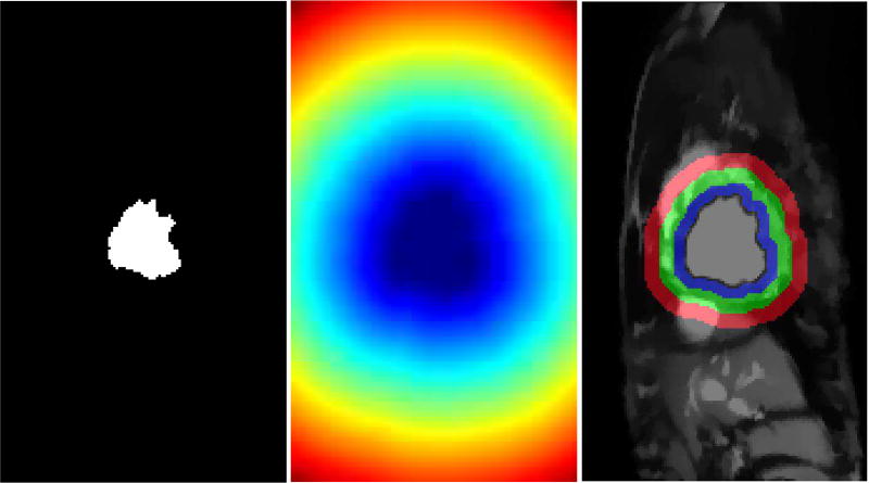
The distance transform from the LV blood pool is used to define two ring-like areas identifying foreground and background regions to sample from as visualized in Fig. 3. In this paper we use a ring thickness of R = 6mm at end systole for all rings involved. In Section IV-C we actually vary this to test robustness. The thicknesses are normalized according to the cardiac phase to ensure that these regions do not include false positives with the following function: $R\frac{f}{f+|f_t-f_{\mathit{\text{ES}}}|}$; where f represents the total number of cardiac phases, f_t represents the frame number of the current phase and f_ES is the end systolic frame. End systolic frame is defined around 30% of the cardiac cycle in accordance with ECG triggering. The regions for foreground M^F (blue ring in Fig. 3) and background M^B (red ring in Fig. 3) will be utilized to draw patch samples to learn the dictionaries.

Fig. 3.

Extracting candidate background and myocardium regions. LV blood pool (left); Distance transform from the LV blood pool boundary (middle); Rudimentary background and foreground classes (right). Only pixels within the blue and red rings (right panel) are used to sample patches for dictionary learning. The green ring acts as boundary in between these two regions to reduce the chance of false positives.

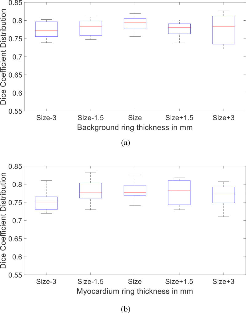
The goal of the last two steps is to obtain a soft definition of where to sample patches from for myocardium and background. Any similar methodology will suffice. Experiments in Fig. 10 show the precision of the last two pre-processing steps does not have a major influence on the performance of the overall algorithm.

Fig. 10.

Effect of Pre-processing on segmentation accuracy. Rudimentary class thickness is varied from the original size (6mm) for background (a) and myocardium (b). The influence of changing the thickness from 3mm to 9mm of both classes on segmentation accuracy is minimal.

B. Dictionary Learning

Learning of per-class dictionaries for segmentation problems is a recent idea also developed in our earlier study [9]. The discriminative dictionary learning idea has been proposed earlier in Atlas-based segmentation of brain MRI [41], [7] and abdominal CT [42] but without the context of motion. However, most methods assume that clear annotation to which class a patch belongs to. Herein we train per-class dictionaries that jointly model appearance and motion that are trained from imprecise data. We expect that the different motion patterns of the myocardium and background and their sparse representation of motion guides the definition of appropriate linear subspaces to capture the variability in the data.

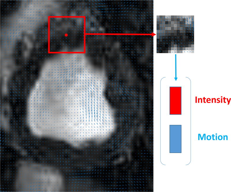
Our method builds observations from the concatenation (after raster-scanning) of square patches of appearance (pixel intensities) and corresponding motion (found via optical flow). Specifically, given (1) a series of pre-processed images I_t, {t = 1 …, T}, (2) the estimated optical flow between subsequent images I_t and I_t+d and (3) the corresponding regions $M_t^F$ and $M_t^B$ obtained as previously described, two matrices were obtained, Y^B and Y^F, where these matrices contain the data from the background and foreground information from the entire cine stack respectively. The j-th column of the matrix Y^F is obtained by concatenating the normalized patch vector of pixel intensities and motion vectors calculated by the method in [43] taken around the j-th pixel in the foreground as shown in Fig. 5. Both horizontal and vertical components are used for each pixel. The Dictionary Learning part of our method takes as input these two matrices Y^B and Y^F, to learn dictionaries D^B, D^F and a sparse feature matrix X^B, X^F.

Fig. 5.

The feature vector generation as concatenation of intensities of square patches and corresponding motion vectors inside that patch.

In order to achieve discriminative initialization, highly correlated data are disregarded prior to learning in a step termed as “intra-class Gram filtering”. In particular, we calculate for a given class C (foreground or background), the intra-class Gram matrix as:

$$G^C=({Y^C)}^T{Y}^C.$$ (1)

We sort the training patches w.r.t. the sum of their related coefficients in the Gram Matrix, and we prune the top 10% of the patches.

Then, dictionaries consisting of K atoms and sparse features with L non-zero elements are trained with K-SVD [44]:

$$\underset{D^F,X^F}{\text{arg min}}\Vert Y^F-D^F{X}^F\Vert \mathrm{s}.\mathrm{t}.\forall i\in M^F,{\Vert x_i^F\Vert }_0\le L,$$

$$\underset{D^B,X^B}{\text{arg min}}\Vert Y^B-D^B{X}^B\Vert \mathrm{s}.\mathrm{t}.\forall i\in M^B,{\Vert x_i^B\Vert }_0\le L$$

To reduce correlation between the dictionaries which is expected to reduce classification errors we perform a second pruning step after K-SVD that removes similar atoms. We define this pruning as “inter-class Gram filtering.” We compute the inter-class Gram matrix as:

$$G^{\mathit{\text{IC}}}={(D^B)}^T(D^F),$$ (2)

and the atoms of each dictionary are sorted according to their cumulative coefficients in G^IC. 10% of the atoms from both dictionaries are discarded to promote particularities of the two different classes. The most correlated atoms from both dictionaries are eliminated with this process. The atoms for foreground and background show strong discriminative power as visualized in Fig. ??B.

To perform this classification, we use the dictionaries, D^B and D^F, previously learnt. The Orthogonal Matching Pursuit (OMP) algorithm [45] is used to compute, the two sparse feature matrices X̂^B and X̂^F for a given sparsity level.

C. MRF based smoothing

In this study, we employ a frame-by-frame MRF strategy [46] across all image pixels to enforce spatial regularization on the final segmentation for each image I_t. The process ensures local smoothness of the classification, which is refined according to the labels. Given the residuals for background R_B and foreground R_F the final segmentation is obtained by minimizing the MRF-based energy functional:

$$E_{\text{MRF}}(I_t)=\sum _{p\in I_t}(V_p(I_p)+\lambda V_{\mathit{\text{pq}}}(I_p,I_q))$$ (3)

where V_p(·) corresponds to the unary potentials representing the data term for node p and V_pq(·) corresponds to the pairwise potentials representing the smoothness term for pixels at nodes p and q in a neighborhood N in the image I_t. The data term measures the disagreement between the prior and the observed data, which is based on the residuals of dictionaries. For a pixel p with initial label C: Label(p) = C, data term is: V_p(I_p) = R^C. The smoothness term is defined as $V_{\mathit{\text{pq}}}(I_p,I_q)=\sum _{q\in N}{R}^{C\prime }$ on the nodes that have different class Label(q) = C′ in the neighborhood N. The parameter λ controls the trade off between smoothness and data term that govern the final segmentation. The smoothness term penalizes discontinuities in a neighborhood N. In our implementation, the total energy is calculated using the residuals for the possible labels of foreground R^F and background R^B. More precisely, if $R^F={\Vert y_i^{\mathit{\text{BF}}}-D^F{\hat{X}}_i^F\Vert }_2$ is larger than $R^B={\Vert y_i^{\mathit{\text{BF}}}-D^B{\hat{X}}_i^B\Vert }_2$, the patch is assigned to the background; otherwise, it is considered belonging to the foreground region for the initial segmentation. The label update occurs if the total energy calculated adding the unary and pairwise terms is smaller for the other label as detailed in Algorithm 1. The method converges either when there is no change of labels or the maximum number of iterations are reached.

IV. Experimental Results

This section offers a qualitative and quantitative analysis of the proposed method, as well as quantitative comparison of our proposed method w.r.t. state-of-the-art methods, to demonstrate its effectiveness for myocardial segmentation.

Our quantitative analysis consists of comparing our method with others and also looking into regional effects and performance. Unless otherwise noted we use 13 × 13 patch size, a dictionary of K = 400 atoms, a sparsity level of L = 4, as parameters. Their influence (and computational performance of our method) are discussed in subsection IV-D.

Data Set

Our set consists of the same 10 canines imaged under four different settings. 2D short-axis images of the whole cardiac cycle with in-plane spatial resolution of 1.25 mm × 1.25 mm were acquired at baseline and severe ischemia (inflicted as controllable stenosis of the left-anterior descending coronary artery (LAD)) on a 1.5T Espree (Siemens Healthcare) along the mid ventricle using both standard CINE and a flow and motion compensated CP-BOLD acquisition within few minutes of each other [2]. In other words we have the same subject matched for each condition and imaging sequence. Thus, we can ascertain by keeping the anatomy fixed the effects of BOLD contrast and presence of disease. Ground truth of myocardial delineations was generated by an expert. Image resolution for the datasets is 192 × 114 with approximately 30 temporal frames (phases).

Algorithm 1.

Proposed Method

Require: Image sequence from single subject
Ensure: Predicted Myocardium masks across the sequence
1:	Calculate Optical Flow fp at each pixel p between pairs of frames (It, It+d)
2:	Generate YB and YF concatenating image intensities and motion information for each patch
3:	for C={B,F} do
4:	Intra-class Gram filtering using 1
5:	Learn dictionary and sparse feature matrix with the K-SVD algorithm $$\underset{D^C,X^C}{\text{minimize}}{\Vert Y^C-D^C{X}^C\Vert }_2^2\mathrm{s}.\mathrm{t}.{\Vert x_i^C\Vert }_0\le L$$
6:	Inter-class Gram filtering using 2
7:	end for
8:	Learn residuals RB and RF given Y, DB and DF with OMP algorithm
9:	Test on all residuals RB and RF for first classification
10:	Use MRF-based segmentation on the residuals RB and RF using Equation 3

Methods of comparison and variants

All quantitative analysis for supervised methods was performed using a strict leave-one-subject-out cross validation. For our implementation of Atlas-based segmentation methods, the registration algorithms dDemons [6] and FFD-MI [20] are used to propagate the segmentation mask of all other subjects to the image of the test subject, followed by a majority voting to obtain the final myocardial segmentation. For supervised classifier-based methods, namely Appearance Classification using Random Forest (ACRF) and Texture-Appearance Classification using Random Forest (TACRF) random forests are used as classifiers to get segmentation labels from different features. To provide more context, we compared our approach with dictionary-based methods, DDLS, RDDL, MSDDL and UMSS. DDLS is an implementation of the method in [7], whereas the discriminative dictionary learning of [47] was used for RDDL. MSDDL [9] uses a multi-scale supervised dictionary learning approach with majority voting classification. UMSS [10] is a unsupervised method relying only on a motion-based coarse segmentation of background. This method learns background class only with a dictionary and performs classification with one-class SVM. Finally, to showcase the strengths of our design choices that contribute to performance of the proposed method, we considered three additional variants of our method (i.e. ablations), without Total Variation pre-processing (Proposed No TV), without Gram filtering (Proposed No Gram Filtering), without concatenating optical flow features with intensity for Dictionary Learning (Proposed No Motion) and without spatial regularization using MRF (Proposed No MRF).

Evaluation Metrics

To evaluate performance we used three metrics, the first two are classically used when evaluating segmentation [48]. We used the Dice overlap measure, which is defined between two regions A and B defined as:

$$D(A,B)=\frac{2\Vert A\cap B\Vert }{\Vert A\Vert \cup \Vert B\Vert }.$$

To evaluate the match of the ground truth annotation to an algorithm’s result in terms of distance, we relied on the Hausdorff distance between two contours C^A and C^B:

$$\mathit{\text{HD}}(C^A,C^B)=\text{max}\{\underset{a\in C^A}{\mathit{\text{max }}}\underset{b\in C^B}{\mathit{\text{min }}}d(a,b),\underset{b\in C^B}{\mathit{\text{min }}}\underset{a\in C^A}{\mathit{\text{max }}}d(a,b)\}$$

where d presents the distance of points a ∈ C^A and b ∈ C^B.

Since part of our analysis is to evaluate how errors in segmentation affect the BOLD response (and its patterns) we use cosine similarity to evaluate the match between two intensity signals S^A, and S^B (e.g. time series) as:

$$\mathit{\text{CS}}=\frac{S^A·S^B}{|S^A||S^B|}$$

where |·| corresponds to ℓ₂ norm of the vector. (We multiply with 100 to report in %.)

A. Comparison with other methods

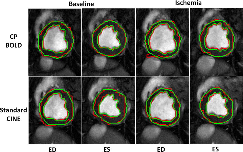
The visual quality of myocardial segmentation by the proposed method for both baseline and ischemia cases across standard CINE and CP-BOLD MR is shown in Fig. 6. The End-diastole (ED) and End-systole (ES) phases are picked as exemplary images from the entire cardiac cycle. Note that our method results in very smooth endo- and epi-cardium contours, which closely follow ground truth contours generated by the experts and can be attributed to the successful representation of myocardial motion.

Fig. 6.

Segmentation result (red) of Proposed method for both CP-BOLD MR and standard CINE MR at baseline and ischemic condition for End-diastole (ED) and End-systole (ES) superimposed with corresponding Manual Segmentation (green) contours delineated by experts.

These observations also hold quantitatively when relying on the Dice metric for evaluation. As Table I shows, overall, for standard CINE, most algorithms perform adequately well and the presence of ischemia slightly reduces performance. However, when BOLD contrast is present, some of the approaches that have not been designed to handle the BOLD contrast lose performance (i.e. those without a ‘*’ in the table). Specifically, Atlas-based methods, ACRF and TACRF are all shown to perform better in standard CINE compared to CP-BOLD. Among dictionary-based methods, DDLS performs well in standard CINE MR, but under-performs in CP-BOLD MR. On the other hand our proposed method performs on par with (and in some cases outperforms) methods that have been designed to handle BOLD contrast (namely MSDDL and UMSS). This is revealing since MSDDL is fully supervised and uses multi-scale features but not motion whereas UMSS albeit being unsupervised and relying on motion uses a single dictionary. It appears that combining motion and using two dictionaries even if they are trained on imprecisely annotated data, is beneficial. Other design choices contribute as well, as comparisons with the proposed method’s variants reveal. In particular, TV-smoothing contributes mostly in extracting more meaningful patterns from optical flow for both CP-BOLD and standard Cine MR.

TABLE I.

Dice coefficient (mean ± std) for myocardial segmentation accuracy in %.

	Baseline		Ischemia
Methods	Standard CINE	CP-BOLD	Standard CINE	CP-BOLD
Atlas-based methods
dDemons [6]	60 ± 8	55 ± 8	56 ± 6	49 ± 7
FFD-MI [20]	60 ± 3	54 ± 8	54 ± 8	45 ± 6
Supervised classifier-based methods
ACRF	57 ± 3	25 ± 2	52 ± 3	21 ± 2
TACRF	65 ± 2	29 ± 3	59 ± 1	24 ± 2
Dictionary-based methods
DDLS [7]	71 ± 2	32 ± 3	66 ± 3	23 ± 4
RDDL [47]	42 ± 15	50 ± 20	48 ± 13	61 ± 12
MSDDL* [9]	75 ± 3	75 ± 2	75 ± 2	71 ± 2
UMSS* [10]	62 ± 20	71 ± 10	65 ± 14	66 ± 11
Proposed unsupervised method
Proposed No TV	65 ± 6	59 ± 7	63 ± 8	57 ± 9
Proposed No Gram Filtering	62 ± 5	52 ± 4	53 ± 5	57 ± 7
Proposed No Motion	71 ± 6	69 ± 8	67 ± 9	68 ± 8
Proposed No MRF	74 ± 5	75 ± 6	73 ± 7	72 ± 6
Proposed	77 ± 10	77 ± 9	74 ± 7	74 ± 6

^*denotes a method that has been designed to handle BOLD contrast.

B. Segmental analysis

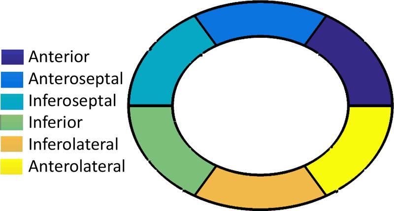
Here we analyze segmentation results by taking into account the spatial distribution of the errors. For each myocardium segmented both manual and automatically, we divide it in 6 radially concentric regions, following the six-segment AHA model for the mid-ventricular slice [49]. Specifically, we take the manually segmented masks and divide them to six radially concentric regions 0°, 60°, 120°, 180°, 240° and 300°. As a reference, a diagram of this process, known as bullbs eye view, is shown in Fig. 7 along with anatomical nomenclature.

Fig. 7.

Six segments of mid-ventricular myocardial slice

Quantitative Analysis

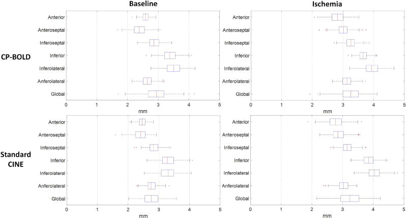
In Fig. 8 boxplots of the Hausdorff distance metric for the epicardium for CP-BOLD and standard CINE MR are presented. Endocardium results show subpixel accuracy on average, and are excluded for brevity. The boxes represent the lower quartile, median and upper quartile values; the whiskers represent the whole extension of the error distribution whereas the crosses correspond to outliers. The global error distribution shows the presence of two outliers, whereas the remaining segmentations have mean errors lower than ≈ 4 mm for images with 1.25 mm spatial resolution. Our reported results of Hausdorff distance are at par with [26]. In the case of Hausdorff distance errors, largest values are located at the inferior region mainly due to the presence of liver.

Fig. 8.

Segmental Hausdorff distance accuracy for CP-BOLD and standard CINE MR for epicardium.

A comparison is shown in Table II to indicate the stability of the method when ischemia is present. The Dice overlap measure is calculated for the 6 regions of the myocardium. In general our algorithm is robust to regional complexities of the myocardium. Ischemia appears to slightly influence the performance especially in the regions that are under influence of LAD stenosis (Anteroseptal, Anterior and Anterolateral).

TABLE II.

Regional segmentation accuracy measured via Dice (mean ± std) in % for Standard CINE and CP-BOLD.

	Baseline		Ischemia
Regions	Std. CINE	CP-BOLD	Std. CINE	CP-BOLD
Anterior	81±13	83±10	78±10	79±8
Anteroseptal	79±10	82±9	75±10	75±9
Inferoseptal	75±12	72±16	75±12	75±9
Inferior	72±11	70±12	69±11	71±8
Inferolateral	73±8	72±12	71±13	71±11
Anterolateral	82±7	81±9	76±11	74±9

Time series analysis for ischemia detection

It is important to evaluate quantitatively the influence of segmentation errors on preserving the BOLD effect to reduce errors of ischemia detection methods [3], [2], [4]. As a benchmark, we used the BOLD signal intensity as obtained via averaging (and normalizing) pixel values in various regions with and without disease obtained from myocardial definitions from ground truth or algorithm results. Fig. 1C already alludes that our proposed approach outperforms other segmentation methods, and this performance also holds when disease is present (see Fig. 9). This also holds quantitatively when comparing with an Atlas-based method [6] as an illustrative example, using the cosine similarity metric (see Table III). Evidently, small errors (even 5–10 pixels) in segmentation towards hyperintense (blood pool) or hypointense (lung/liver interface) areas when a myocardial region is as small as 100 pixels in systole have severe effects in preserving the BOLD signal.

Fig. 9.

Normalized time series obtained by averaging pixel intensities in the anterior region, as defined using ground truth (blue) and automatic segmentation (red dotted line) in a subject at baseline (left) and after LAD stenosis and during ischemia (right). Observe that the time series obtained via the proposed segmentation is consistent with that of ground truth, which eventually result in more accurate ischemia detection.

TABLE III.

Cosine Similarity comparison of Timeseries of 6-segmental regions (mean ± std, in %) acquired from the ground truth compared with the proposed method and Atlas-based method [6] for CP-BOLD sequences.

	Proposed		Atlas-based [6]
Regions	Baseline	Ischemia	Baseline	Ischemia
Anterior	93±2	89±3	89±4	86±5
Anteroseptal	92±5	83±6	89±5	81±8
Inferoseptal	82±5	83±9	80±8	80±11
Inferior	79±4	80±8	75±8	77±11
Inferolateral	81±3	80±9	81±3	80±9
Anterolateral	91±3	83±5	88±5	81±7

C. Segmentation performance across cardiac phases

Since our approach uses motion patterns as input features, it is interesting to evaluate if natural changes in cardiac motion affect performance. We evaluated this by measuring performance over different cardiac phases (early diastole to late systole) of the cardiac cycle in Table IV. We partitioned the cardiac cycle to four phases as early diastole, late diastole, early systole and late systole according to ECG triggering. First and last points in the R-R interval correspond to diastole, whereas systole appear around 30%. Overall the performance of the algorithm is consistent throughout the cardiac cycle as anticipated given that dictionaries are learned by pooling patches across the entire cardiac sequence.

TABLE IV.

Dice coefficient (mean ± std) for myocardial segmentation accuracy in % of different cardiac stages.

	Baseline		Ischemia
Stage	Std. CINE	CP-BOLD	Std CINE	CP-BOLD
Early diastole	76 ± 5	76 ± 6	73 ± 4	75 ± 4
Late diastole	75 ± 4	75 ± 4	74 ± 6	73 ± 7
Early systole	77 ± 5	77 ± 3	75 ± 7	74 ± 6
Late systole	78 ± 4	78 ± 6	75 ± 4	75 ± 5

D. Parameter analysis and computational performance

The purpose of this section is to analyze effects of different parameters of the algorithm as well as discuss computational performance. First we evaluate pre-processing; then patch size, number of atoms K, and sparsity level L varying one of the 3 but keeping the other two fixed using the following values: patch size of 13 × 13, K = 400 and L = 4.

Influence of pre-processing

Pre-processing consists of identifying both background and myocardium regions to sample from, which depend on the thickness of the rings that define them. Here we vary this ring size (from the initial size of 6mm) keeping all other parameters fixed. Fig. 10 illustrates that the results remain consistent whether modifying more the background (more false negatives) or the myocardium (more false positives) class. This result demonstrates that we can tolerate imprecision in defining the regions to sample from.

Influence of patch size

The patch size is related to the local geometry whilst the neighborhood size reflects the anatomical variability. The Dice coefficient distributions over varying patch are presented in Fig. 11a for a dictionary size of K = 400 atoms, and sparsity of L = 4. As one can observe, the best median Dice coefficient was obtained with a patch size of 13 × 13 albeit it performed similar to 15 × 15. This is to be expected as this comes close to the average size of the myocardium given the image size of our dataset.

Fig. 11.

Effect of patch size (a), dictionary size (b) and sparsity threshold (c) on segmentation accuracy. The optimal results were obtained using a patch size of 13 × 13, a dictionary of 400 atoms and a sparsity threshold of 4.

Influence of dictionary size and sparsity level

First, experiments were carried out to study the influence of dictionary size K (the number of atoms in each dictionary) on segmentation accuracy with fixed values 13 × 13 patch size and L = 4 sparsity threshold. As illustrated by Fig. 11b, 400 atoms provide a good balance of accuracy w.r.t. dictionary size. Note that a larger dictionary does imply higher computational complexity, albeit it also depends on sparsity level.

Thus, experiments were also carried out to study the influence of the sparsity level L (the number of non-zero components in sparse coefficients) on segmentation accuracy. This governs the selection of atoms to be combined for the purpose of representing classes with the dictionaries. Fig. 11c shows that sparsity 4 is the most suited level of sparsity for our experiments and indicates the importance of this parameter. It appears that lower sparsity has higher discriminative ability as adding additional atoms it appears to add noisy information.

Computational Complexity

Execution time on a 2.4 GHz processor with an average data set (192 × 114 × 30) is approximately seven minutes. Most of this time is spent on the dictionary learning stage (approx. 4 minutes).

V. Discussion

Cardiac MRI is an emerging modality in the management of cardiovascular disease. Its ability to obtain multiple contrasts that can be used to ascertain various degrees and complexities of pathology makes it a powerful diagnostic tool. For example, the CP-BOLD sequence used in this study is such a sequence that can obtain information on myocardial status (ischemia) and function (motion). However, this flexibility comes at a cost for the required post-processing. This study clearly showed that algorithms developed to segment the myocardium in Standard CINE MRI severely under-perform when applied to images from CP-BOLD studies. It showed that new algorithms are necessary for accurate segmentation, and the proposed algorithm aims to segment the myocardium in CP-BOLD without any supervision in a fully automated fashion.

The results show that the unsupervised automatic segmentation resulting from the proposed method results in an acceptable level of agreement with manual segmentations. The main challenge of CP-BOLD data stems from spatio-temporal variations of the myocardial signal. We address this in several ways. First we reduce the BOLD effect by variational temporal smoothing which has not been applied as pre-processing before in the context of cardiac BOLD data. We then use both appearance and motion for dictionary learning. Different from others we train these dictionaries from data that have uncertainty in their annotation and these data are subject-specific. Finally, since classification based on residuals may lead to non-smooth contours locally, we use MRFs to obtain the final segmentation. As experiments on time series comparisons showed, accurate segmentation translates directly to the fidelity of the signal that we aim to preserve, namely: BOLD contrast. This will have direct effects on fully automated ischemia detection [4].

This study used 2D (+time) datasets at mid-ventricular slice; however when 3D BOLD approaches become routinely available it will be interesting to see how the presented method extends to 3D. We envision that iterating the steps of training the dictionaries and segmentation could be beneficial, as with more accurate class definitions the discriminative power of the dictionaries is increased. In addition, it is possible that we can exploit data augmentation to perhaps learn better features. Another avenue of improvement will be the thickness normalization function of the preprocessing scheme, which relies on a fixed estimate currently.

In conclusion, this study motivates us to rethink the standard assumptions and verification metrics regarding the segmentation of the myocardium in cardiac MRI. Development of MR technologies bring new challenges and departing from fully supervised techniques (the performance of which heavily depends on the amount of training data) towards unsupervised ones can provide multiple benefits. Finally, this work has shown that global DICE score on its own is not a sufficient performance metric and more analysis can bring about the suitability of segmentation methods for particular MR techniques.

References

- 1.Dharmakumar R, Arumana JM, Tang R, Harris K, Zhang Z, Li D. Assessment of regional myocardial oxygenation changes in the presence of coronary artery stenosis with balanced SSFP imaging at 3.0T: Theory and experimental evaluation in canines. JMRI. 2008;27(5):1037–1045. doi: 10.1002/jmri.21345. [DOI] [PubMed] [Google Scholar]
- 2.Tsaftaris SA, Zhou X, Tang R, Li D, Dharmakumar R. Detecting myocardial ischemia at rest with Cardiac Phase-resolved Blood Oxygen Level-Dependent Cardiovascular Magnetic Resonance. Circ. Cardiovasc. Imaging. 2013;6(2):311–319. doi: 10.1161/CIRCIMAGING.112.976076. [DOI] [PMC free article] [PubMed] [Google Scholar]
- 3.Tsaftaris SA, Tang R, Zhou X, Li D, Dharmakumar R. Ischemic extent as a biomarker for characterizing severity of coronary artery stenosis with blood oxygen-sensitive MRI. JMRI. 2012;35(6):1338–1348. doi: 10.1002/jmri.23577. [DOI] [PMC free article] [PubMed] [Google Scholar]
- 4.Bevilacqua M, Dharmakumar R, Tsaftaris SA. Dictionary-driven ischemia detection from cardiac phase-resolved myocardial BOLD MRI at rest. IEEE TMI. 2016;35(1):282–293. doi: 10.1109/TMI.2015.2470075. [DOI] [PMC free article] [PubMed] [Google Scholar]
- 5.Oksuz I, Mukhopadhyay A, Bevilacqua M, Dharmakumar R, Tsaftaris SA. Dictionary learning based image descriptor for myocardial registration of CP-BOLD MR. MICCAI. 2015:205–213. [Google Scholar]
- 6.Vercauteren T, Pennec X, Perchant A, Ayache N. Non-parametric Diffeomorphic Image Registration with the Demons Algorithm. MICCAI. 2007;4792:319–326. doi: 10.1007/978-3-540-75759-7_39. [DOI] [PubMed] [Google Scholar]
- 7.Tong T, Wolz R, Coup P, Hajnal JV, Rueckert D. Segmentation of MR images via discriminative dictionary learning and sparse coding: Application to hippocampus labeling. NeuroImage. 2013;76:11–23. doi: 10.1016/j.neuroimage.2013.02.069. [DOI] [PubMed] [Google Scholar]
- 8.Tsaftaris SA, Andermatt V, Schlegel A, Katsaggelos AK, Li D, Dharmakumar R. A dynamic programming solution to tracking and elastically matching left ventricular walls in cardiac cine MRI. 2008:2980–2983. [Google Scholar]
- 9.Mukhopadhyay A, Oksuz I, Bevilacqua M, Dharmakumar R, Tsaftaris SA. Data-driven feature learning for myocardial segmentation of CP-BOLD MRI. FIMH. 2015:189–197. [Google Scholar]
- 10.Mukhopadhyay A, Oksuz I, Bevilacqua M, Dharmakumar R, Tsaftaris SA. Unsupervised myocardial segmentation for cardiac MRI. MICCAI. 2015:12–20. doi: 10.1109/TMI.2017.2726112. [DOI] [PMC free article] [PubMed] [Google Scholar]
- 11.Petitjean C, Dacher J-N. A review of segmentation methods in short axis cardiac MR images. MedIA. 2011;15(2):169–184. doi: 10.1016/j.media.2010.12.004. [DOI] [PubMed] [Google Scholar]
- 12.Peng P, Lekadir K, Gooya A, Shao L, Petersen SE, Frangi AF. A review of heart chamber segmentation for structural and functional analysis using cardiac magnetic resonance imaging. Magn. Reson. Mater. Phy. 2016;29(2):155–195. doi: 10.1007/s10334-015-0521-4. [DOI] [PMC free article] [PubMed] [Google Scholar]
- 13.Jolly M-P, Xue H, Grady L, Guehring J. Combining registration and minimum surfaces for the segmentation of the left ventricle in cardiac cine MR images. MICCAI. 2009:910–918. doi: 10.1007/978-3-642-04271-3_110. [DOI] [PubMed] [Google Scholar]
- 14.Lin X, Cowan BR, Young AA. Automated detection of left ventricle in 4D MR images: Experience from a large study. MICCAI. 2006:728–735. doi: 10.1007/11866565_89. [DOI] [PubMed] [Google Scholar]
- 15.Pednekar A, Kurkure U, Muthupillai R, Flamm S, Kakadiaris I. Automated left ventricular segmentation in cardiac MRI. IEEE TBE. 2006;53(7):1425–1428. doi: 10.1109/TBME.2006.873684. [DOI] [PubMed] [Google Scholar]
- 16.Cordero-Grande L, Vegas-Sanchez-Ferrero G, Casaseca-de-la Higuera P, Alberto San-Roman-Calvar J, Revilla-Orodea A, Martn-Fernandez M, Alberola-Lopez C. Unsupervised 4D myocardium segmentation with a Markov random field based deformable model. MedIA. 2011;15(3):283–301. doi: 10.1016/j.media.2011.01.002. [DOI] [PubMed] [Google Scholar]
- 17.Cai Y, Islam A, Bhaduri M, Chan I, Li S. Unsupervised freeview groupwise cardiac segmentation using synchronized spectral network. IEEE TMI. 2016;35(9):2174–2188. doi: 10.1109/TMI.2016.2553153. [DOI] [PubMed] [Google Scholar]
- 18.Bai W, Shi W, O’Regan DP, Tong T, Wang H, Jamil-Copley S, Peters NS, Rueckert D. A Probabilistic Patch-Based Label Fusion Model for Multi-Atlas Segmentation With Registration Refinement: Application to Cardiac MR Images. IEEE TMI. 2013;32(7):1302–1315. doi: 10.1109/TMI.2013.2256922. [DOI] [PubMed] [Google Scholar]
- 19.Bai W, Shi W, Ledig C, Rueckert D. Multi-atlas segmentation with augmented features for cardiac MR images. MedIA. 2015;19(1):98–109. doi: 10.1016/j.media.2014.09.005. [DOI] [PubMed] [Google Scholar]
- 20.Glocker B, Komodakis N, Tziritas G, Navab N, Paragios N. Dense image registration through MRFs and efficient linear programming. MedIA. 2008;12(6):731–741. doi: 10.1016/j.media.2008.03.006. [DOI] [PubMed] [Google Scholar]
- 21.Zhen X, Wang Z, Islam A, Bhaduri M, Chan I, Li S. Direct estimation of cardiac bi-ventricular volumes with regression forests. MICCAI. 2014:586–593. doi: 10.1007/978-3-319-10470-6_73. [DOI] [PubMed] [Google Scholar]
- 22.Huang X, Dione DP, Compas CB, Papademetris X, Lin BA, Bregasi A, Sinusas AJ, Staib LH, Duncan JS. Contour tracking in echocardiographic sequences via sparse representation and dictionary learning. MedIA. 2014;18(2):253–271. doi: 10.1016/j.media.2013.10.012. [DOI] [PMC free article] [PubMed] [Google Scholar]
- 23.Hu H, Liu H, Gao Z, Huang L. Hybrid segmentation of left ventricle in cardiac MRI using gaussian-mixture model and region restricted dynamic programming. JMRI. 2013;31(4):575–584. doi: 10.1016/j.mri.2012.10.004. [DOI] [PubMed] [Google Scholar]
- 24.Lynch M, Ghita O, Whelan P. Segmentation of the left ventricle of the heart in 3-D+t MRI data using an optimized nonrigid temporal model. IEEE TMI. 2008;27(2):195–1203. doi: 10.1109/TMI.2007.904681. [DOI] [PubMed] [Google Scholar]
- 25.Paragios N. A variational approach for the segmentation of the left ventricle in cardiac image analysis. IJCV. 2002;50(3):345–362. [Google Scholar]
- 26.Queiros S, Barbosa D, Heyde B, Morais P, Vilaa JL, Friboulet D, Bernard O, Dhooge J. Fast automatic myocardial segmentation in 4D cine CMR datasets. MedIA. 2014;18(7):1115–1131. doi: 10.1016/j.media.2014.06.001. [DOI] [PubMed] [Google Scholar]
- 27.Eslami A, Karamalis A, Katouzian A, Navab N. Segmentation by retrieval with guided random walks: Application to left ventricle segmentation in MRI. MedIA. 2013;17(2):236–253. doi: 10.1016/j.media.2012.10.005. [DOI] [PubMed] [Google Scholar]
- 28.Lombaert H, Cheriet F. Spatio-temporal segmentation of the heart in 4D MRI images using graph cuts with motion cues. ISBI. 2010 [Google Scholar]
- 29.Spottiswoode BS, Zhong X, Lorenz CH, Mayosi BM, Meintjes EM, Epstein FH. Motion-guided segmentation for cine dense MRI. MedIA. 2009;13(1):105–115. doi: 10.1016/j.media.2008.06.016. [DOI] [PMC free article] [PubMed] [Google Scholar]
- 30.Avendi M, Kheradvar A, Jafarkhani H. A combined deep-learning and deformable-model approach to fully automatic segmentation of the left ventricle in cardiac MRI. MedIA. 2016;30:108119. doi: 10.1016/j.media.2016.01.005. [DOI] [PubMed] [Google Scholar]
- 31.Ngo TA, Lu Z, Carneiro G. Combining deep learning and level set for the automated segmentation of the left ventricle of the heart from cardiac cine magnetic resonance. MedIA. 2017;35:159–171. doi: 10.1016/j.media.2016.05.009. [DOI] [PubMed] [Google Scholar]
- 32.Tran PV. A fully convolutional neural network for cardiac segmentation in short-axis mri. arXiv: 1604.00494. 2016 [Google Scholar]
- 33.Cicek A, Abdulkadir O, Lienkamp SS, Brox T, Ronneberger O. 3d U-net: Learning dense volumetric segmentation from sparse annotation. MICCAI. 2016:424–432. [Google Scholar]
- 34.Tan LK, Liew YM, Lim E, McLaughlin RA. Convolutional neural network regression for short-axis left ventricle segmentation in cardiac cine mr sequences. MedIA. 2017;39:78–86. doi: 10.1016/j.media.2017.04.002. [DOI] [PubMed] [Google Scholar]
- 35.Litjens G, Kooi T, Bejnordi BE, Setio AAA, Ciompi F, Ghafoorian M, van der Laak JA, van Ginneken B, Sánchez CI. A survey on deep learning in medical image analysis. arXiv preprint arXiv: 1702.05747. 2017 doi: 10.1016/j.media.2017.07.005. [DOI] [PubMed] [Google Scholar]
- 36.Rudin LI, Osher S, Fatemi E. Nonlinear total variation based noise removal algorithms. Physica D: Nonlinear Phenomena. 1992;60(1–4):259268. [Google Scholar]
- 37.Mukhopadhyay A. Total variation random forest: Fully automatic MRI segmentation in congenital heart diseases. RAMBO-HVSMR. 2016 [Google Scholar]
- 38.Chan SH, Khoshabeh R, Gibson KB, Gill PE, Nguyen TQ. An augmented lagrangian method for total variation video restoration. IEEE TIP. 2011;20(11):3097–3111. doi: 10.1109/TIP.2011.2158229. [DOI] [PubMed] [Google Scholar]
- 39.Guillemaud R, Brady M. Estimating the bias field of MR images. IEEE TMI. 1997;16(3):238–251. doi: 10.1109/42.585758. [DOI] [PubMed] [Google Scholar]
- 40.Otsu N. A threshold selection method from gray-level histograms. Automatica. 1975;11(285–296):23–27. [Google Scholar]
- 41.Benkarim OM, Radeva P, Igual L. Label consistent multiclass discriminative dictionary learning for MRI segmentation. Articulated Motion Deformable Objects. 2014:138–147. [Google Scholar]
- 42.Tong T, Wolz R, Wang Z, Gao Q, Misawa K, Fujiwara M, Mori K, Hajnal JV, Rueckert D. Discriminative dictionary learning for abdominal multi-organ segmentation. MedIA. 2015;23(1):92–104. doi: 10.1016/j.media.2015.04.015. [DOI] [PubMed] [Google Scholar]
- 43.Brox T, Bruhn A, Papenberg N, Weickert J. High accuracy optical flow estimation based on a theory for warping. 2004:25–36. [Google Scholar]
- 44.Aharon M, Elad M, Bruckstein A. K–SVD: An Algorithm for Designing Overcomplete Dictionaries for Sparse Representation. IEEE TSP. 2006;54(11):4311–4322. [Google Scholar]
- 45.Tropp JA, Gilbert AC. Signal recovery from random measurements via orthogonal matching pursuit. IEEE TIT. 2007;53(12):4655–4666. [Google Scholar]
- 46.Besbes A, Komodakis N, Paragios N. Graph-based knowledge-driven discrete segmentation of the left ventricle. ISBI. 2009:49–52. [Google Scholar]
- 47.Ramirez I, Sprechmann P, Sapiro G. Classification and clustering via dictionary learning with structured incoherence and shared features. 2010 [Google Scholar]
- 48.Radau LY, Connelly PK, Paul G, Dick A WG. Evaluation framework for algorithms segmenting short axis cardiac mri. MIDAS Journal. 2009 [Google Scholar]
- 49.Cerqueira MD, Weissman NJ, Dilsizian V, Jacobs AK, Kaul S, Laskey WK, Pennell DJ, Rumberger JA, Ryan T, Verani MS. Standardized myocardial segmentation and nomenclature for tomographic imaging of the heart. Circulation. 2002;105(4):539–542. doi: 10.1161/hc0402.102975. [DOI] [PubMed] [Google Scholar]