A Continuum Poisson-Boltzmann Model for Membrane Channel Proteins

Abstract

Membrane proteins constitute a large portion of the human proteome and perform a variety of important functions as membrane receptors, transport proteins, enzymes, signaling proteins, and more. Computational studies of membrane proteins are usually much more complicated than those of globular proteins. Here we propose a new continuum model for Poisson-Boltzmann calculations of membrane channel proteins. Major improvements over the existing continuum slab model are as follows:1) The location and thickness of the slab model are fine-tuned based on explicit-solvent MD simulations. 2) The highly different accessibility in the membrane and water regions are addressed with a two-step, two-probe grid labeling procedure, and 3) The water pores/channels are automatically identified. The new continuum membrane model is optimized (by adjusting the membrane probe, as well as the slab thickness and center) to best reproduce the distributions of buried water molecules in the membrane region as sampled in explicit water simulations. Our optimization also shows that the widely adopted water probe of 1.4 Å for globular proteins is a very reasonable default value for membrane protein simulations. It gives the best compromise in reproducing the explicit water distributions in membrane channel proteins, at least in the water accessible pore/channel regions that we focus on. Finally, we validate the new membrane model by carrying out binding affinity calculations for a potassium channel, and we observe a good agreement with experiment results.

Introduction

Membrane proteins constitute a large portion of the human proteome and perform a variety of important functions, such as membrane receptors, transport proteins, enzymes, and signaling proteins¹. These important proteins have become primary drug targets in modern medicine: over 60% of all drugs target these proteins^2-4. However, the study of membrane proteins is usually much more complicated than that of globular proteins, both experimentally and computationally. For experimental studies, the difficulty of obtaining a high-resolution structure is an obstacle, especially for studies that involve proteins found in humans. For computational studies, modeling of the membrane environment is also an important consideration.

Since most biomolecular systems exist in an aqueous environment, it is important to account for solvent effects. There are two ways to include solvent effects in a computational simulation: explicit and implicit solvation. In explicit solvation modeling, each solvent atom is modeled explicitly. Although this is the most accurate method, what we are interested in is often not the properties of the solvent itself, but rather its influence on the solute molecules. In addition, accurately capturing the solvent influence in a statistically meaningful way requires sampling either from an ensemble of trajectories or from a single very long trajectory, which is very computationally demanding. Implicit solvation modeling provides an attractive alternative wherein the solvent molecules are collectively modeled as a continuum. In implicit solvent models, although the details of individual solvent atoms are lost, the relevant important statistically averaged effects can still be preserved by design. Since solvent molecules typically constitute the major portion of molecules for an explicit solvent simulation, implicit solvent modeling can lead to much more efficient simulations^5-21. In addition to water, membrane molecules should also be included when modeling solvation effects, and implicit membrane modeling has also been developed^22-28.

A key issue in developing implicit solvent models is the modeling of electrostatic interactions. The Poisson-Boltzmann equation (PBE) has been established as a fundamental equation to model continuum electrostatic interactions^29-47. The solvent molecules are modeled as a continuum with a high dielectric constant, and the solute atoms are modeled as a continuum with a low dielectric constant and buried atomic charges. The effect of charged ions in the solvent region is included by adding mobile charge density terms that obey Boltzmann distributions. The potential of the full system is then governed by the partial differential equation:

$$\nabla \cdot \epsilon \nabla \varphi =-4\pi {\rho }_0-4\pi \sum _{i}e{z}_i{c}_i\lambda exp(-e{z}_i\varphi /k_{B}T)$$ (1)

where ∇ is the spatial gradient operator, ε is the dielectric constant distribution, ϕ is the electrostatic potential distribution, ρ₀ is the charge density of the solute (usually modeled as a set of discrete point charges), c_i is the concentration of the ith solvent ion species in bulk, e is the absolute charge of an electron, z_i is the valence for the ith ion, k_B is Boltzmann's constant, T is the temperature, and is the Stern layer masking function, which is 0 within or 1 outside of the Stern layer.

The PBE is a non-linear elliptical partial differential equation, with closed form solutions only for very simple geometries. Numerical solutions are required for biomolecular applications due to their complex shapes^{22, 36, 44, 45, 48-87}. Efficient numerical PBE-based solvent models have been widely used to study biological processes including predicting pKa values^88-91, computing salvation and binding free energies^92-101, and protein folding^102-112. Predicting protein-ligand binding affinities is one of the major applications for implicit solvent free energy calculations. In the Amber software package, MMPBSA is the module performing such calculations ^113-118. Implicit membrane modeling has also been applied and developed in binding free energy calculations. There are a noticeable number of pioneer works that implement implicit membrane modeling in several PB packages, such as APBS ²⁷, Delphi ^{28, 119}, PBEQ^{78, 120}, and PBSA^121-123. All of them add the membrane as a slab with a relatively low dielectric constant that is embedded in water for PBE calculations.

Our previous work implemented an implicit membrane model into the PBE framework¹²¹. The implicit membrane model can be readily interfaced with the existing MMPBSA program^113-118 to perform binding free energy calculations of several protein structures embedded in a membrane^{87, 124}. However, a problem arises when those membrane proteins contain a pore or a gated channel, since the region of the channel is usually permeable and should be composed of water. Therefore, a simple slab-like membrane setup may cause problems if the membrane protein contains pore- or channel-like region(s). Similar to the approaches adopted in the community^{28, 119, 125}, we dealt with this issue by manually defining the pore region as a cylinder, and we then set the dielectric constant within the cylindrical region as that of water if it was not occupied by protein atoms, for example as in DelPhi that allows for multiple dielectric constant regions of membrane^{28, 119, 125}. The limitation of this method is that, for every snapshot of a trajectory, we need to visualize and locate the cylinder by hand, which is neither efficient nor practical given the large number of snapshots that must be processed for converged calculations.

In this work, we propose a new continuum membrane model for PBE calculations of biomolecules. Major improvements from the existing continuum slab model are the following:1) an explicit solvent MD simulation was exploited to fine tune the slab model, i.e. its exact location and thickness, to best reproduce the solvent accessibility and the water accessible channel, 2) a two-step, two-probe initial grid labeling procedure was adopted to address highly different accessibility in the membrane region and water region, and 3) a depth-first search algorithm was introduced to detect the water pores/channels automatically based on the initial grid labels. This procedure follows our basic algorithm proposed for globular proteins, and adds little overall overhead in the application of linear finite-difference PBE solvers to typical membrane proteins.

Methods

The Poisson-Boltzmann equation (Eqn (1)) is widely used in capturing electrostatic energy and forces in implicit solvent modeling. For systems with dilute ion concentrations, the second term on the right-hand side is usually linearized, giving the simpler form:

$$\nabla \cdot \epsilon \nabla \varphi =-4\pi {\rho }_0+\lambda {\kappa }^2\varphi$$ (2)

where ${\kappa }^2=4\pi \sum _i{c}_i{e}_i^2{z}_i^2/k_{B}T$.

The finite-difference method^{22, 43, 71-83, 86} is one of the most popular methods used in the numerical implementation of the PBE. In a typical procedure, the rectangular grid covering the solution system is first defined. Next, the atomic point charges are mapped onto grid points with a predefined assignment function. Third, the dielectric constant distribution is mapped to grid edges. The discretized linear system is then turned to a linear solver to solve for potentials on grid points, which can be expressed as:

$${\epsilon }_x(i-1,j,k)\varphi (i-1,j,k)+{\epsilon }_x(i,j,k)\varphi (i+1,j,k)+{\epsilon }_y(i,j-1,k)\varphi (i,j-1,k)+{\epsilon }_y(i,j,k)\varphi (i,j+1,k)+{\epsilon }_z(i,j,k-1)\varphi (i,j,k-1)+{\epsilon }_z(i,j,k)\varphi (i,j,k+1)-({\epsilon }_x(i-1,j,k)+{\epsilon }_x(i,j,k)+{\epsilon }_y(i,j-1,k)+{\epsilon }_y(i,j,k)+{\epsilon }_z(i,j,k-1)+{\epsilon }_z(i,j,k))\varphi (i,j,k)+h^2\lambda (i,j,k){\kappa }^2\varphi (i,j,k)=-\frac{4\pi \rho (i,j,k)}{h}$$ (3)

Here ϕ(i,j,k), ρ(i,j,k), and λ(i,j,k) are the potential, the charge, and the Stern masking function at grid point (i,j,k), respectively. Other indexing notations for ϕ are defined similarly. ε_x, ε_y, and ε_z represent the dielectric constants for grid edges along the x, y, and z directions, respectively. Specifically ε_x(i-1,j,k) is the dielectric constant at the mid-point between grid points (i-1,j,k) and (i,j,k). Other indexing notations for ε_x, ε_y, ε_z are defined similarly. Finally h represents the grid spacing.

This study focuses on how to set up linear PBE applications for membrane systems. A major issue is the presence of the membrane and its influence on the dielectric constant distribution. In globular proteins, the solvent excluded surface (SES)^{43, 126-130} is often used as a boundary separating the high dielectric water exterior and the low dielectric protein interior. The presence of the membrane introduces at least a third region. In this study, we adopt the uniform membrane dielectric model, though our procedure can be easily extended to accommodate another often used depth-dependent membrane dielectric model.

The first step is to introduce a membrane region to the existing solvent excluded surface procedure with minimum invasion to the program and minimum efficiency lost. The SES is the most common surface definition used to describe the dielectric interface between the two piece-wise dielectric constants. In fact, comparative analysis of PB-based solvent models and TIP3P solvent models have shown that the SES definition is reasonable in the calculation of reaction field energies and electrostatic potentials of mean force fields.^131-133 Here, we follow the idea from Rocchia et al.¹³⁰ and Wang et al.⁴³ of mapping the SES to a finite-difference grid. While keeping the variables used to label the solvent and solute regions, we also introduce a new variable to label the membrane region. Considering the membrane lipid molecules are usually larger than solvent molecules, we use two different solvent probe radii to set up the membrane and solvent regions. And finally, we assign the dielectric constant on each region and the interface.

Grid point labeling

Our general strategy is to model the membrane as a second continuum solvent of finite region, i.e. a slab located at a user specified position. The essence of the algorithm is to determine both the membrane accessibility and water accessibility around a molecular solute. Assisted with both sets of accessibility data, the presence of water channels or water pores within the membrane region can then be identified in the next step. Due to the much larger size of lipid molecules, a separate solvent probe ( mprob) must be used to determine the membrane accessibility. This is apparently much larger than the water probe ( dprob). The influence of both probes on reproducing the solvent accessible surface of a membrane protein is presented in Results and Discussion.

In Amber/PBSA, an integer array insas is used to label whether the grid point is outside the solute region ( insas<0) or inside the solute region ( insas>0) for fast mapping of solvent accessibility information as shown in Figure 1. This labeling scheme has been extended to map all commonly used surfaces, SES, Solvent-Accessible Surface (SAS), van der Waals Surface (VDW), and Density Function Surface (DEN) in recent Amber and AmberTools releases^{36, 43, 80, 82, 87, 134, 135}. To minimize the interference to existing procedures and maximize efficiency, a separate integer array inmem is used to label whether a grid point is inside the membrane ( inmem>0) or outside the membrane ( inmem=0). Specifically, the grid-labeling algorithm can be summarized as the following five steps:

• 0Initialize insas of all grid points as “−4”, i.e. in the bulk solvent and salt region, and inmem of all grid points as “0”, i.e. outside the membrane region.
• 1Using mprob as the solvent probe radius, label insas of all grid points as “−3” if within the Stern layer; “−2” if within the solvent accessible surface layer; “−1” if within the reentry region but outside the SES; “1” if within the reentry region but inside the SES; “2” if inside the VDW surface.
• 2Add a slab perpendicular to the z-axis as the membrane region at the specified location. Label inmem of the membrane-region grid points with insas<0 as “1”.
• 3Apply the depth-first search algorithm to detect any possible membrane accessible grid point that is not connected to the bulk membrane. If so, relabel its inmem as “0”.
• 4For each grid point with ( inmem=0) within the slab, if it has a neighbor with ( inmem=1) within the distance cutoff of memmaxd, relabel its inmem as “2”.
• 5Using dprob as the solvent probe radius, relabel insas of all grid points as “-3” if within the Stern layer; “-2” if within the solvent accessible surface layer; “-1” if within the reentry region outside the SES; “1” if within the reentry region inside the SES; “2” if inside the VDW surface.

Figure 1.

Grid point labeling scheme in the numerical SES surface definition. Here -4 stands for grid points in the bulk solvent; -2 stands for grid points within SAS spheres if not overwritten below; 2 stands for grid points within VDW spheres; 1 stands for grid points within bicones (shown as the fine dashed triangles) formed by overlapping SAS spheres if not overwritten below; -1 stands for grid points accessible to solvent probes placed on the solvent accessible arcs that are formed by overlapping SAS spheres. The Stern lay is omitted for clarity.

A few explanations are in order here. First, inmem is determined in Step 2 through Step 4, so that its value is controlled by both the mprob-generated insas and the depth-first search algorithm. Second, a new variable ( memmaxd) is introduced in Step 4. Since mprob is usually much larger than dprob, there exists a thin layer of grid points with insas>0 and inmem=0 between the membrane region and the protein region. If the grid labels are set this way, these grid points would be labeled as water in a later processing stage of our method, thus leading to an artificial layer of water between the protein and membrane. To resolve this issue, a cutoff distance of memmaxd is introduced to represent the maximum difference between the SES surfaces generated by mprob and dprob. This is estimated to be mprob–dprob assuming maximum reentry by dprob. Thus Step 4 changes the inmem labels of the grid points from 0 ( mprob inaccessible) to 2 ( mprob accessible) if they are memmaxd inside the mprob-generated SES. The correction effectively removes the artificial layer of water between the protein and the membrane. Here the revised inmem values are set to be“2” so these grid points would not interfere with the subsequent search. Note too that this correction does not change the protein interior definition, which is defined with the water dprob. Nevertheless, it does have the effect of pushing back the potential buried water pockets, if any, from the protein-membrane interface.

In summary, there are three different regions readily available for further processing after the grid-labeling step:

1. Solute region: insas (i, j, k) >0

2. Membrane region: insas (i, j, k) <0 and inmem (i, j, k)>0

3. Solvent region: insas (i, j, k) <0 and inmem(i, j, k)=0

Membrane pore/channel detection

Step 3 in the above general grid-labeling algorithm is meant to identify pore- or channel-like water-accessible water pockets within a user-specified membrane region. Given the convention that the membrane is parallel with the xy plane, the membrane region can be mathematically defined to be all grid points within [ zmin, zmax]. Thus the method starts by initializing all grid points that are defined as solvent ( insas<0) within [ zmin, zmax] as inmem=1. Next the recursive depth-first search algorithm is used to traverse all grid points to see whether they are connected or not. Our goal of using the algorithm is to walk and label recursively all grid points in the non-protein regions within [ zmin, zmax]. Upon completion, all grid points that are not connected to the membrane region (i.e. the pore region) are labeled back as the water region ( inmem=0). The detail of the algorithm is summarized in Appendix A.1.

Mapping solvent/membrane accessibility to dielectric constants

In this study, we adopted a three-dielectric model to model the membrane-protein electrostatics. The dielectric constants for the three different regions are denoted as ε_in (solute), ε_out (solvent) and ε_mem (membrane), respectively.

The general principle to map the grid labeling information into the dielectric constants is that the dielectric constant of a grid edge should be equal to the dielectric constant in the region where the two flanking grid points reside, consistent with our original approach for globular proteins as described in Wang et al ⁴³. When the two neighboring grid points belong to different dielectric regions, the weighted harmonic averaging (WHA) method is used to calculate the “fractional” dielectric constant based on the precise intersection point where the molecular surface cut the grid edge⁴³. Specifically the dielectric constant is assigned as:

$$\epsilon =\frac{1}{\frac{a}{{\epsilon }_1}+\frac{1-a}{{\epsilon }_2}},$$ (5)

where a denotes the fraction of the grid edgein region 1. Eqn (5) is applied on three different kinds of interfaces:

$$\begin{array}{cc}{\epsilon }_1={\epsilon }_{\mathit{\text{in}}},{\epsilon }_2={\epsilon }_{\mathit{\text{out}}}& \text{solute and solvent interface}\\ {\epsilon }_1={\epsilon }_{\mathit{\text{in}}},{\epsilon }_2={\epsilon }_{\mathit{\text{mem}}}& \text{solute and membrane interface}\\ {\epsilon }_1={\epsilon }_{\mathit{\text{out}}},{\epsilon }_2={\epsilon }_{\mathit{\text{mem}}}& \text{solvent and membrane interface}\end{array}$$ (6)

Overall the grid edges can be classified according to the rules summarized in Table I. The assignment of dielectric constants on the solute and water interface is the same as Wang et al⁴³. The assignment of dielectric constants on the membrane related region and interface is summarized in Appendix A.2. In summary, all the edges in the water region are assigned the dielectric constant of water, all the edges in the membrane region are assigned the dielectric constant of membrane, and all the edges in the protein interior are assigned the dielectric constant of protein. For all the edges across different regions, i.e. between any two of water, membrane, or protein, weighted harmonic averages between the two corresponding dielectric constants are assigned.

Table I.

Different edges of dielectric constants defined by adjacent values of insas and inmem.

insas(i,j,k)	insas(i+1,j,k)	inmem(i,j,k)	inmem(i+1,j,k)	region
>0	>0	>0	>0	inside solute
>0	>0	>0	=0	inside solute
>0	>0	=0	>0	inside solute
>0	>0	=0	=0	inside solute
>0	<0	>0	>0	solute and membrane interface
>0	<0	>0	=0	solute and solvent interface
>0	<0	=0	>0	solute and membrane interface
>0	<0	=0	=0	solute and solvent interface
<0	>0	>0	>0	solute and membrane interface
<0	>0	>0	=0	solute and membrane interface
<0	>0	=0	>0	solute and solvent interface
<0	>0	=0	=0	solute and solvent interface
<0	<0	>0	>0	inside membrane
<0	<0	>0	=0	inside solvent
<0	<0	=0	>0	inside solvent
<0	<0	=0	=0	inside solvent

Protein and complex structure preparation

To calibrate the new continuum membrane model for channel detection, we simulated three channel proteins with crystal structures: 1K4C ¹³⁶, a KcsA potassium channel; 5CFB ¹³⁷, an alpha1 GlyR Glycine receptor; and 5HCJ ¹³⁸, a prokaryotic pentameric ligand-gated ion channel. To demonstrate the feasibility of the new continuum membrane model in data intensive binding affinity calculations, we chose the hERG K⁺ channel protein, given its importance in drug discovery and the availability of high-quality experimental data ¹³⁹.

Unfortunately crystal structure for the hERG K⁺ channel does not exist, so a homology model in the closed state was built based on the crystal structure of KcsA (PDB ID: 1K4C)¹³⁶. The amino acid sequence of the hERG K⁺ channel was directly extracted from the Swiss-Prot database ¹⁴⁰ (accession number: Q12809 and entry: KCNH2_HUMAN). Given the low sequence homology, we followed the published protocol to conduct sequence alignment and homology modeling¹⁴¹. Specifically, the alignment was first constructed based on the sequence homologies involving pore helices and S5 and S6 helices that have been confirmed in the literature^141-145. The final alignment was generated using CLUSTALX (version 2.1)^141-146, showing a good match in helices S5, S6, and the pore region, with identity about 44% (Figure 2). After automatic model building and loop refinement, candidate models were evaluated based on the DOPE score from MODELLER (version 9.15)^{141-145, 147}. The final homology model of the hERG K⁺ channel is shown in Figure 3, which is found to be highly consistent with a previously reported homology model based on a slightly different procedure ^{143, 148-150}.

Figure 2.

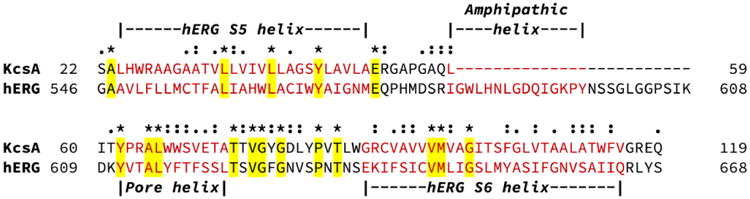
Sequence alignment of KcsA and hERG by ClustalX version 2.1. The identified S5 helix, S6 helix, amphipathic helix and pore helix are labeled above the sequence. Asterisks (*): conserved amino acid residues; colons (:): conserved substitutions; dots (.): semi-conserved substitutions.

Figure 3.

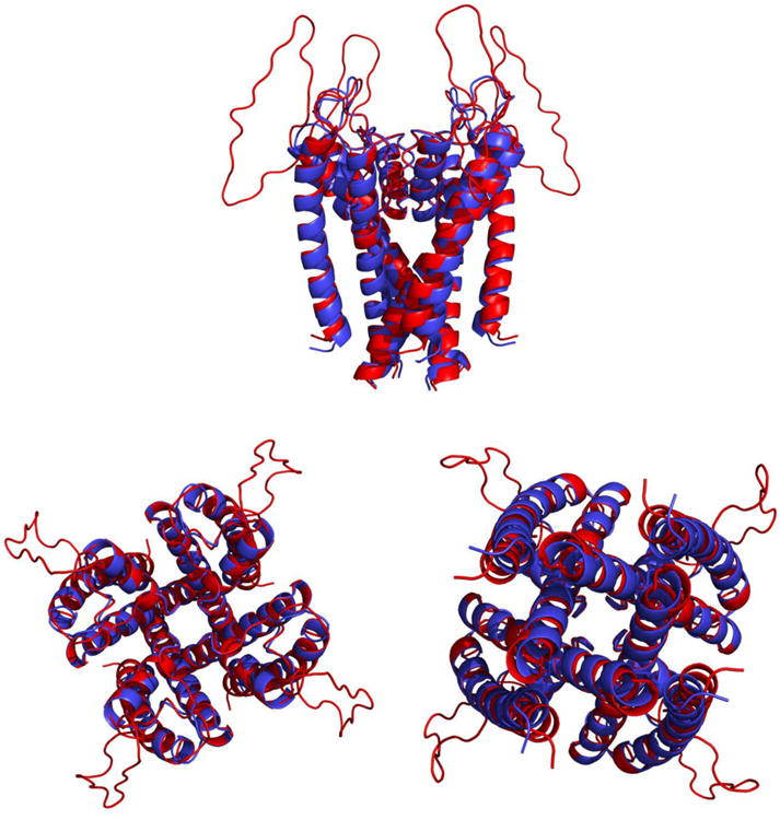
Comparison of target and parent structures, showing the secondary structure elements in homology models of hEGH (red) and KcsA (blue). The plot shows three orientations of the aligned structure. Top: side view with the binding pocket on the top. Bottom left: view from the binding pocket/extracellular side. Bottom right: view from the intracellular side.

Initial complex structures of the hERG K⁺ channel with its inhibitors were generated with the surflex-dock program in Sybyl-X (version 1.3). Ten different inhibitors with experimental binding affinities¹³⁹ were chosen to assess the quality of the MMPBSA procedure, including astemizole (AST), sertindole (SER), pimozide (PIM), droperidol (DRO), terfenadine (TE0,TE1), domperidone (DOM), loratadine (LOR), mizolaatine (MIZ), perhexiline (PE0, PE1) and amitriptyline (AMI). The terfenadine and perhexiline are chiral molecules with two enantiomers, so both enantiomers were used in the docking.

Molecular dynamics simulation

The protein was first inserted into a membrane layer using the CHARMM-GUI lipid builder^151-155. Lipid DPPC was used for the membrane layer with a lipid to water ratio of29. The solvated membrane system first underwent a 10,000-step energy minimization using a 5,000-step steepest descent followed by a 5,000-step conjugate gradient. The main chain atoms for the protein were then restrained with a force constant of 2 kcal/mol-Ų. Subsequently, a 5 ps MD simulation was conducted to heat the system from 0 to 100K followed by a 100 ps MD simulation to heat the system from 100K to 310K. This was then followed with a 5 ns simulation for equilibration. Finally, production MD was run for 50 ns.

MMPBSA calculations of binding affinities

Binding free energies were computed using a revised MMPBSA module¹²⁴ of Amber 16 or AmberTools 2016^{134, 135, 156}. The production run trajectory was post-processed with CPPTRAJ¹⁵⁷ in order to remove the solvent, membrane, and counter ions from the receptor-ligand complex. Snapshots from the last 10 ns of the production run were processed to compute molecular mechanics potential energies and solvation free energies in the MMPBSA procedure. The binding free energy for the protein-ligand complex was computed as the difference between the complex free energy and the sum of the receptor and ligand free energies, as outlined in our previous work¹²⁴. The electrostatic solvation free energies were calculated using the linearized PBE model as implemented in PBSA^{36, 43, 80, 82, 87}. The non-electrostatic solvation free energies were calculated using either the classical model or the modern model as documented previously¹⁵⁸.

Additional computational details

In each PBSA calculation, a finite-difference grid spacing of 0.5 Å was used for MMPBSA calculations, which was found to be sufficient due to MD sampling and the approximate nature of the binding affinity calculation¹¹⁸. Production snapshots up to 10ns were found to be sufficient to converge the averaging process used in MMPBSA calculations of these membrane protein-ligand complexes. The periodic geometric multigrid solver option was employed with a convergence threshold of 1.0 × 10^-3, and electrostatic focusing was turned off due to the presence of the membrane⁸⁷. The use of a periodic boundary also allowed a somewhat small fillratio (i.e. the ratio of the finite-difference box dimension over the solute dimension) of 1.25 to be used in these calculations³⁷. The solvation system physical constants were set up as follows. The membrane was modeled as a continuum slab as simulated in the explicit water MD trajectories. The water relative dielectric constant was set at 80.0. The membrane dielectric constant was set to be 7.0 ¹²⁴. And the protein dielectric constant was set to be 20.0 due to the presence of charged ligand molecules ^{118, 124}. The water phase ionic strength was set to be 150 mM. The lower dielectric region within the molecular solutes was defined with the classical solvent excluded surface model using a water solvent probe and a membrane solvent probe to be optimized as described in Results and Discussion. The default weighted harmonic averaging was employed to assign dielectric constants for boundary grid edges to reduce grid dependency⁴³. Charges and radii were assigned as in the simulation topology files.

Results and Discussion

Optimization of the new slab membrane model

Given the automatic procedure in place to identify water channels/pores with the depth-first search method, we further optimized the membrane probe value and the slab membrane model (i.e. its thickness) to best reproduce the distributions of buried water molecules in the membrane region as sampled in explicit water MD simulations. Three different membrane proteins with channels were utilized in this optimization: 1K4C, 5HCJ, and 5CFB.

Three different slab definitions were evaluated to set up the continuum membrane model, i.e. the inner and outer faces are chosen to be positioned at (1) the average z-coordinates of nitrogen atoms of the lipid head groups; (2) the average z-coordinates of the phosphorus atoms of the lipid head groups; (3) the average z-coordinates of both nitrogen and phosphorus atoms in the lipid head groups. Here the average z-coordinates are computed from the explicit-water MD simulations.

Next, mprob values were scanned from 1.4 Åupwards to 3.0 Å with an increment of 0.1 Å. The smallest mprob value with which these known channels can be displayed was recorded as the mprob threshold in Table II for all three slab membrane definitions. It should be pointed out that a small mprob produces excessive membrane accessibility in the protein interior so that it is more likely for the buried membrane pockets to be connected to the bulk membrane. Excessive membrane accessibility can also be lessened by reducing the membrane thickness, as in the use of phosphorus atoms to define the boundaries of the continuum membrane. Indeed, our analysis showed this setup caused the least penetration of the continuum membrane into the protein interior, so the smallest mprob (2.7 Å) was needed to capture the water channels/pores for all three tested proteins.

Table II.

The thickness of membrane and mprob thresholds based on the different criterion measured from MD simulations. Here the mprob threshold is the minimum value with which the channel is visible with the SES approach. (Top) mthick=|N⁺–N⁻|: The thickness of the membrane slab is defined as the z-distance between the average head group nitrogen atoms of the lipid molecules. (Middle) mthick=|P⁺–P⁻|: The thickness of the membrane slab is defined as the z-distance between the average head group phosphorus atoms of the lipid molecules. (Bottom) mthick=|N⁺P⁺– N⁻P⁻|: the membrane slab is defined as the z-distance between the average head group centers (i.e. the means of nitrogen and phosphorus atoms) of the lipid molecules. The membrane center locations were then computed as the mean of the upper and lower bounds.

Protein	mthick (Å)	mcenter(Å)	mprob (Å)
	mthick=|N+–N−|
1K4C	39.24	-1.10	>2.2
5CFB	40.72	64.95	>1.7
5HCJ	41.11	68.60	>3.0
	mthick=|P+–P−|
1K4C	36.13	-0.97	>2.2
5CFB	37.27	64.97	>1.6
5HCJ	37.89	68.40	>2.7
	mthick=|N+P+– N−P−|
1K4C	37.69	-1.04	>2.2
5CFB	39.00	64.96	>1.7
5HCJ	39.50	68.50	>3.0

Figure 4 shows the rendering of water-channels/pores of the three tested membrane proteins with the optimized mprob. The SI movies available online provide a more detailed view for each of the three channel proteins rendered in 3D. The advantage of the optimal mprob over the default solvent probe of 1.4 Å is apparent by comparing the renderings generated with the two probes. For all the channel proteins, the new model automatically detects the water channels/pores. Figure 5 further shows the benefit of the depth-first-search feature that is a must in the new slab membrane model. Without it, it is apparent that none of the water channels/pores can be identified for any of the tested proteins, even using the larger probe for the membrane region.

Figure 4.

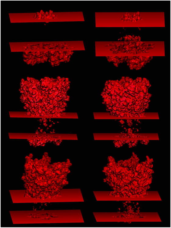
Solvent-solute interface determined with the new continuum membrane model. Left:mprob is set to be 1.4 Å, the default value of the solvent probe. Right: mprob is set to be 2.7 Å, the optimized value of the membrane probe. Three proteins are tested: 1K4C (top); 5CFB (middle); 5HCJ (bottom).

Figure 5.

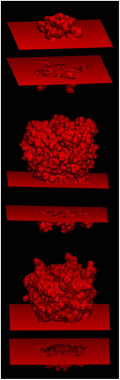
Same as the right panel with the optimized mprob in Figure 3, except without turning on the depth-first search in the pore region detection. Three proteins are tested: 1K4C (top); 5CFB (middle); 5HCJ (bottom).

Impact of the water solvent probe upon agreement with an explicit solvent simulation

It is worth pointing out that the agreement of the continuum membrane model also depends on how we model the water accessible region. The standard practice has been to consider the finite size of the water molecule with a predefined probe radius, often taken as 1.4 Å. The probe is then used to compute the solvent excluded surface used as the interface separating the protein interior from the water region. It is apparent that the size of the water accessible pores/channels would depend on how large the water probe is defined. Thus, it is interesting to analyze how well the widely used water probe performs in the context of membrane channel proteins.

This analysis was conducted in the following manner. The distributions of water molecules (in the water pore/channel regions) in explicit water MD simulations were sampled every 50 ps over the course of a 5 ns production run. Note that the protein atoms were all restrained to the reference structure after equilibration since the focus was on the water distribution. A total of 100 frames worth of water sampling were collected and were combined into one snapshot for visualization. This water distribution map was used as a reference to evaluate how the hard sphere SES surface behaves with one single adjustable parameter, i.e. the water solvent probe ( dprob in Amber/PBSA).

The same three membrane channel proteins were analyzed to address this question. Specifically, the counts for the following disagreements/mismatches were recorded: (1) the absence of explicit water molecules in the continuum water accessible regions; and (2) the presence of explicit water molecules in the continuum water inaccessible regions. The overall summary of both mismatches is reported in Table III. Sample mismatches are shown in Figure 6. It is interesting to note that the standard value of the water solvent probe of 1.4Å is a very reasonable default value, which gives the best compromise between the two competing effects. That is if the probe is too small, there are too many regions without water density where water molecules were detected in the MD simulations, while if the probe is too large, there are too many regions with water density.

Table III.

Discrepancies in the solvent accessible region between explicit water MD simulations and the membrane PBSA calculations. Two types of discrepancies were recorded: (1) how many continuum solvent pockets do not have water molecules; and (2) how many explicit water molecules are observed in the non-continuum solvent pockets defined in the membrane PBSA calculation. The water probe (dprob)was scanned from 1.2 Å to 1.6 Åfor three different proteins: 1K4C, 5CFB, and 5HCJ. The membrane setup has been optimized according to the values given in Table II. For each protein, the samples of water molecules were taken from a 5 ns equilibrium MD simulation with all protein atoms restrained to the initial structure. This was obtained from the last snapshot of the unconstrained normal MD, which is also the reference for the water sampling run. The listed values are the averages of 100 snapshots evenly selected from the 5ns MD simulation.

Protein	dprob(Å)	No. solvent region w/o water molecules	No. water molecules in non-solvent region
1K4C	1.2	23	4
	1.3	18	8
	1.4	15	11
	1.5	14	14
	1.6	12	15
5CFB	1.2	20	5
	1.3	17	10
	1.4	14	11
	1.5	10	17
	1.6	7	22
5HCJ	1.2	22	4
	1.3	18	7
	1.4	9	11
	1.5	9	17
	1.6	7	23

Figure 6.

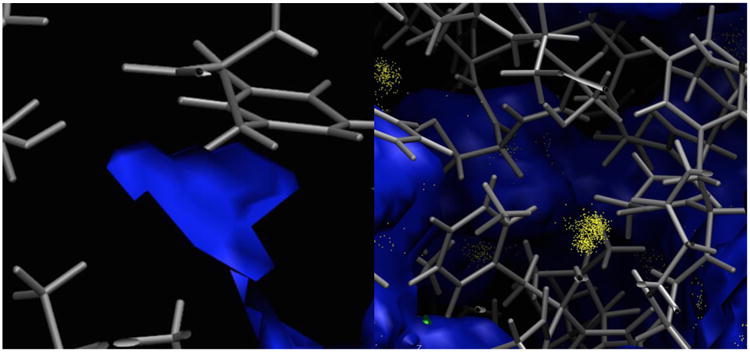
Discrepancy between implicit and explicit water simulations. The protein surface of 1K4C (blue) is overlaid with a bond representation and sampled water positions (yellow). Left: a solvent region defined by the PBSA model but with no explicit water. Right: explicit water is detected in a region where no solvent is defined in the PBSA model.

It is instructive to point out that the inconsistency between the two representations may be due to the setup of the explicit water MD simulation and also to the limitations of MD sampling of water distributions. First, it is well known that isolated water cavities exist in the protein interior, which are disconnected from the bulk water. Unless crystal water molecules were observed and retained in the initial setup of the MD simulations, these isolated cavities are most likely modeled as water-free due to the default closeness tolerance used in the placement of explicit water molecules when building the topology files. This issue would lead to the type (1) mismatches described above.

Second, although protein atoms were restrained during the MD simulations, they are not as inflexible as frozen hard spheres as in the case of the continuum solvent model that must use a single mean structure as input. Their motions allow minor structural changes, leading to the opening and closing of buried water cavities. If the mean structure happens to correspond to a closed form, the continuum model would not capture the water-accessible cavity.

Finally, the protein atom cavity radii that were used to present the size of each atom were chosen to be best for energetics and/or stability of the MD simulations. These may or may not be optimal to quantify water accessibility in the protein interior. This points to future efforts to model the protein-water interface more self-consistently based on the consistent energy model as defined by the protein-water force field used in both explicit and implicit simulations.

MMPBSA calculations of binding affinities

Finally, as an illustration of our automatic continuum membrane model, we conducted a set of binding free energy calculations of ten different ligands independently bound to a potassium channel protein. The computed binding affinities and experimental IC₅₀ values are summarized in Table IV. The correlation analysis between computation and experiment is shown in Figure 7. Both the classical and modern nonpolar solvent models ¹⁵⁸(INP=1, where the overall nonpolar solvation free energy is computed as a term linearly dependent on the molecular surface; and INP=2, where the dispersion/van der Waals component is numerically integrated assuming a uniform solvent distribution and the hydrophobic/cavity component is computed as a term linearly dependent on the molecular surface or the molecular volume) were tested, and the correlations for these two methods are similar, which is consistent with what we expected. Overall good correlations with experiment were observed: with correlation coefficients of 0.79 for INP=1 and 0.73 for INP=2 (due to the smaller range of the data).

Table IV.

MMPBSA binding affinities (kcal/mol)in comparison with experiment (IC₅₀). The slab membrane geometry (the thickness and z-centerin Å) compiled from the explicit solvent MD simulation are also shown for each complex.

Name	RTln(IC50)	mthick	mcenter	MMPBSA (INP=1)	MMPBSA (INP=2)
Amitriptyline	-7.08	36.086	-10.383	-38.23	-9.84
Perhexline (PE0)	-7.23	36.661	-1.620	-40.73	-12.44
Perhexline (PE1)	-7.23	36.473	-5.681	-41.96	-13.63
Mizolastine	-9.15	36.260	1.360	-61.25	-24.59
Loratadine	-9.58	36.126	-0.969	-52.48	-18.64
Domperidone	-9.62	35.979	0.707	-59.53	-20.69
Terfenadine (TE0)	-9.82	36.616	-2.319	-69.67	-29.00
Terfenadine (TE1)	-9.82	37.216	-0.611	-72.91	-30.56
droperidol	-10.61	36.459	3.308	-59.04	-24.78
Pimozide	-10.97	36.910	0.190	-60.04	-20.09
Sertindole	-11.13	36.438	-1.161	-62.91	-23.89
Astemizole	-12.81	34.133	-0.043	-67.64	-26.21

Figure 7.

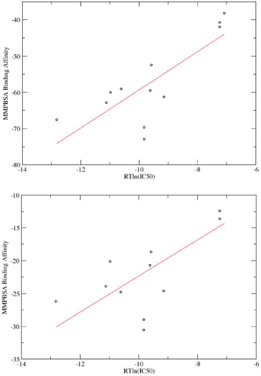
MMPBSA binding affinities compared with experimental measurements. Binding affinities are in kcal/mol. Top: MMPBSA was computed with the classical nonpolar solvent model (INP=1);the correlation coefficient is 0.79. Bottom: MMPBSA was computed with the modern nonpolar solvent model (INP=2); the correlation coefficient is 0.73.

Note also that we have used a high protein dielectric constant of 20 because portion of the ligand molecules are charged and the rest are neutral. Our previous studies have shown that a high protein dielectric constant best reproduces experimental results in MMPBSA calculations when charged ligands/active sites present in globular proteins^{118, 124}. A similar conclusion can also be drawn in the tested membrane protein: when the “default” protein dielectric value of 4 is used, the correlation is reduced from 0.79 to 0.75 with INP=1. The high protein dielectric is a reasonable but crude treatment to account for the screened electrostatic interactions due to electronic, orientational, and solvent-exchange polarization as in pKa calculations by the PB models. Typical MD simulations utilized for MMPBSA calculations are apparently insufficient for sampling all the orientational and solvent-exchange polarization. Electronic polarization is also missing in widely used additive force fields. Thus this strategy is still a useful approximation for rapid MMPBSA calculations of binding interactions. However, the use of a high protein dielectric constant does have a side effect of downplaying electrostatic effects in binding interactions. Thus the effect of pores/channels would play a less important role in the electrostatic interactions due to this set up for the specific system.

Timing analysis

Finally, we conducted a timing analysis of the new membrane model. Table V summarizes the average CPU times over 100 frames that are used for setting up the dielectric grids with or without the membrane model in the MMPBSA calculation of the receptor. We can see the average time for the surface calculation increases by more than four times; this is mainly because two separate SES calls are made, once with the water probe and once with the membrane probe. Furthermore, the SES calculation with the much larger membrane probe is behind the much higher cost in the total SES time due to the longer non-bonded list and many more overlaps among larger probe-augmented atomic volumes. In addition, the grid-labeling step is also about three times slower, though not a significant portion of the overall CPU cost. Finally, the mapping from grid labels to dielectric constants changes little due to the virtually linear nature of the algorithm⁴³. Overall the PBSA calculations are about 25% slower with the new continuum membrane model than those without any continuum membrane (i.e. modeled as a globular protein) for the tested protein-ligand binding calculations.

Table V.

Average CPU times (in seconds) used in setting up the dielectric grid for 100 snapshots in the MMPBSA calculation of the receptor. The membrane-free set up was run using memopt=0, and the membrane setup was run using memopt=1 in Amber/PBSA.

	Globular Protein Setup	Membrane Protein Setup
SES Calculations (s)	3.76	15.63
Grid Labeling (s)	1.61	4.79
EPS Mapping (s)	0.21	0.22

Conclusions

We have proposed a new continuum membrane model for Poisson-Boltzmann calculations of biomolecules. Major improvements from the standard continuum slab model are the following:1) explicit-solvent MD simulations were utilized to fine tune the slab model, i.e. its exact location and thickness, to best reproduce the solvent accessibility and the water accessible channel; 2) A two-step, two-probe initial grid labeling procedure was adopted to address highly different accessibility in the membrane region and water region;and 3) A depth-first search algorithm was introduced to detect the water pores/channels automatically based on the initial grid labels. This procedure follows our basic algorithm proposed for globular proteins and does not add significant overhead to the numerical PB calculations.

Given the revisions proposed above, we optimized the membrane probe value and the slab membrane model (i.e. its thickness) to best reproduce the distributions of buried water molecules in the membrane region as sampled in explicit water MD simulations. Three different membrane proteins with channels were utilized in this optimization. Our analysis showed that a slab membrane model using the mean phosphate atom positions as the membrane boundary and the smallest membrane probe of 2.7 Å caused the least penetration of the continuum membrane into the protein interior.

Apparently, the solvent accessibility also depends on how the continuum water is modeled. Thus, we used a water distribution map from an explicit water MD simulation as benchmark data to evaluate how the hard sphere SES behaves with one single adjustable parameter, i.e. the water solvent probe. The same three membrane channel proteins were analyzed to address this question. It is interesting to note that the standard value for the water solvent probe of 1.4Å is very reasonable, which gives the best compromise between the two competing effects.

Finally, we conducted a set of binding affinity calculations of ten different ligands independently bound to a potassium channel using the new continuum membrane model. Both the classical and modern nonpolar solvent models were tested, and the correlations with experiment are similar with both models, which is consistent with our findings in globular proteins. Overall good correlations with experiment were observed, with correlation coefficients of 0.79 for INP=1 and 0.73 for INP=2. Finally, our timing analysis showed that the average time for the surface calculation increased by more than four times. The grid-labeling step is also about three times slower even though it is not a significant portion of the overall CPU cost. The mapping from grid labels to dielectric constants changed little due to the virtually linear nature of the algorithm.

Future efforts will be conducted to model the protein-water interface more self-consistently based on the consistent energy model as defined using the protein-water force field in both explicit and implicit simulations.

A.1 Depth-first Search Algorithm

To facilitate the bookkeeping of the search, the variable kzone is introduced to label the different regions: the protein region ( kzone=0), the membrane region ( kzone=1), and the water regions ( kzone>1). Since the search starts from the edge of the membrane slab, the first region found is always the membrane region ( kzone=1), and the rest are the water regions or the protein region. In general multiple kzone values are assigned because most water-accessible regions are not connected.

nzone = 0; kzone = −1

for k = zmin:zmax

 for j,i = 1:n

  if kzone(i,j,k) != -1 then

   cycle

  end if

  if insas(i,j,k) > 0 then

    kzone(i,j,k) = 0

  else

    nzone = nzone + 1

    kzone(i,j,k) = nzone

   call walk(i,j,k, kzone, nzone)

  end if

 end

end

recursive subroutine walk(i,j,k, kzone, nzone)

  kzone(i,j,k) = nzone

 if ( kzone(i+1,j,k) == −1 .and. insas(i+1,j,k)<0)

 call walk(i+1,j,k, kzone,nzone)

 if ( kzone(i−1,j,k) == −1 .and. insas(i−1,j,k)<0)

 call walk(i−1,j,k, kzone,nzone)

 if ( kzone(i,j+1,k) == −1 .and. insas(i,j+1,k)<0)

 call walk(i,j+1,k, kzone,nzone)

 if ( kzone(i,j−1,k) == −1 .and. insas(i,j−1,k)<0)

 call walk(i,j−1,k, kzone,nzone)

 if (k+1<= zmax .and. kzone(i,j,k+1) == −1 .and. insas(i,j,k+1)<0)

 call walk(i,j,k+1, kzone,nzone)

 if (k−1>= zmin .and. kzone(i,j,k−1) == −1 .and. insas(i,j,k−1)<0)

 call walk(i,j,k−1, kzone,nzone)

end recursive subroutine walk

In this way, all grid points with kzone>1 are water accessible, and inmem of these grid points are set back to 0, i.e. membrane inaccessible.

A.2 Dielectric Constant Assignment

The procedure of assigning the dielectric constants on the membrane related region and interface is as follows:

For x-edges, fractional membrane edges are only possible with the membrane- solute interface, so that the following pseudo code can be added to the existing dielectric mapping procedure:

If ( inmem(i,j,k)>0 .or. inmem(i+1,j,k)>0) then

 If ( insas(i,j,k)>0 .and. insas(i+1,j,k)>0) then

$${\epsilon }_x(i,j,k)={\epsilon }_{\mathit{\text{in}}}$$

 // grid edge in solute

 else if (( insas(i,j,k)>0 .and. inmem(i+1,j,k)>0) .or. ( insas(i+1,j,k)>0 .and. inmem(i,j,k)>0) ) then

$${\epsilon }_x(i,j,k)=\frac{1}{\frac{a}{{\epsilon }_{\mathit{\text{in}}}}+\frac{1-a}{{\epsilon }_{\mathit{\text{mem}}}}}$$

 // grid edge between membrane and solute

 else if ( insas(i,j,k)>0 .or. insas(i+1,j,k)>0) then

$${\epsilon }_x(i,j,k)=\frac{1}{\frac{a}{{\epsilon }_{\mathit{\text{in}}}}+\frac{1-a}{{\epsilon }_{\mathit{\text{out}}}}}$$

 // grid edge between solvent and solute

 else if( inmem(i,j,k)>0 .and. inmem(i+1,j,k)>0) then

$${\epsilon }_x(i,j,k)={\epsilon }_{\mathit{\text{mem}}}$$

 // grid edge in membrane

 end if

end if

Here a is the fraction of grid edge in the solute region. The algorithm along the y-axis is similar to the x-axis, as follows:

If ( inmem(i,j,k)>0 .or. inmem(i,j+1,k)>0) then

 If ( insas(i,j,k)>0 .and. insas(i,j+1,k)>0) then

$${\epsilon }_y(i,j,k)={\epsilon }_{\mathit{\text{in}}}$$

 // grid edge in solute

 else if (( insas(i,j,k)>0 .and. inmem(i,j+1,k)>0) .or. ( insas(i,j+1,k)>0 .and. inmem(i,j,k)>0) ) then

$${\epsilon }_y(i,j,k)=\frac{1}{\frac{a}{{\epsilon }_{\mathit{\text{in}}}}+\frac{1-a}{{\epsilon }_{\mathit{\text{mem}}}}}$$

 // grid edge between membrane and solute

 else if ( insas(i,j,k)>0 .or. insas(i,j+1,k)>0) then

$${\epsilon }_y(i,j,k)=\frac{1}{\frac{a}{{\epsilon }_{\mathit{\text{in}}}}+\frac{1-a}{{\epsilon }_{\mathit{\text{out}}}}}$$

 // grid edge between solvent and solute

 else if( inmem(i,j,k)>0 .and. inmem(i,j+1,k)>0) then

$${\epsilon }_y(i,j,k)={\epsilon }_{\mathit{\text{mem}}}$$

 // grid edge in membrane

 end if

end if

For the dielectric constant mapping along the z-axis, the algorithm also involves the solvent-membrane interface; the algorithm should also take care of this, as follows:

If ( inmem(i,j,k)>0 .or. inmem(i,j,k+1)>0)

 If ( insas(i,j,k)>0 .and. insas(i,j,k+1)>0) then

$${\epsilon }_z(i,j,k)={\epsilon }_{\mathit{\text{in}}}$$

 else if (( insas(i,j,k)>0 .and. inmem(i,j,k+1)>0) .or. ( insas(i,j,k+1)>0 .and. inmem(i,j,k)>0) ) then

$${\epsilon }_z(i,j,k)=\frac{1}{\frac{a}{{\epsilon }_{\mathit{\text{in}}}}+\frac{1-a}{{\epsilon }_{\mathit{\text{mem}}}}}$$

 // grid edge between membrane and solute

 else if ( insas(i,j,k)>0 .or. insas(i,j,k+1)>0) then

$${\epsilon }_z(i,j,k)=\frac{1}{\frac{a}{{\epsilon }_{\mathit{\text{in}}}}+\frac{1-a}{{\epsilon }_{\mathit{\text{out}}}}}$$

 // grid edge between solvent and solute

 else if( inmem(i,j,k)>0 .and. inmem(i,j,k+1)>0) then

$${\epsilon }_z(i,j,k)={\epsilon }_{\mathit{\text{mem}}}$$

 else if (grid edge is cross the slab)

$${\epsilon }_z(i,j,k)=\frac{1}{\frac{a}{{\epsilon }_{\mathit{\text{out}}}}+\frac{1-a}{{\epsilon }_{\mathit{\text{mem}}}}}$$

 // grid edge cross the slab

 // a is fraction of edge in solvent

 end if

end if

References

- 1.Almen MS, Nordstrom KJV, Fredriksson R, Schioth HB. Mapping the human membrane proteome: a majority of the human membrane proteins can be classified according to function and evolutionary origin. Bmc Biol. 2009;7:50. doi: 10.1186/1741-7007-7-50. [DOI] [PMC free article] [PubMed] [Google Scholar]
- 2.Arinaminpathy Y, Khurana E, Engelman DM, Gerstein MB. Computational analysis of membrane proteins: the largest class of drug targets. Drug Discov Today. 2009;14:1130–1135. doi: 10.1016/j.drudis.2009.08.006. [DOI] [PMC free article] [PubMed] [Google Scholar]
- 3.Yildirim MA, Goh KI, Cusick ME, Barabasi AL, Vidal M. Drug-target network. Nat Biotechnol. 2007;25:1119–1126. doi: 10.1038/nbt1338. [DOI] [PubMed] [Google Scholar]
- 4.Overington JP, Al-Lazikani B, Hopkins AL. Opinion - How many drug targets are there? Nat Rev Drug Discov. 2006;5:993–996. doi: 10.1038/nrd2199. [DOI] [PubMed] [Google Scholar]
- 5.Davis ME, Mccammon JA. Electrostatics in Biomolecular Structure and Dynamics. Chem Rev. 1990;90:509–521. [Google Scholar]
- 6.Honig B, Sharp K, Yang AS. Macroscopic Models Of Aqueous-Solutions - Biological And Chemical Applications. J Phys Chem. 1993;97:1101–1109. [Google Scholar]
- 7.Honig B, Nicholls A. Classical Electrostatics in Biology and Chemistry. Science. 1995;268:1144–1149. doi: 10.1126/science.7761829. [DOI] [PubMed] [Google Scholar]
- 8.Beglov D, Roux B. Solvation of complex molecules in a polar liquid: An integral equation theory. J Chem Phys. 1996;104:8678–8689. [Google Scholar]
- 9.Cramer CJ, Truhlar DG. Implicit solvation models: Equilibria, structure, spectra, and dynamics. Chem Rev. 1999;99:2161–2200. doi: 10.1021/cr960149m. [DOI] [PubMed] [Google Scholar]
- 10.Bashford D, Case DA. Generalized born models of macromolecular solvation effects. Annual Review Of Physical Chemistry. 2000;51:129–152. doi: 10.1146/annurev.physchem.51.1.129. [DOI] [PubMed] [Google Scholar]
- 11.Baker NA. Improving implicit solvent simulations: a Poisson-centric view. Curr Opin Struct Biol. 2005;15:137–143. doi: 10.1016/j.sbi.2005.02.001. [DOI] [PubMed] [Google Scholar]
- 12.Chen JH, Im WP, Brooks CL. Balancing solvation and intramolecular interactions: Toward a consistent generalized born force field. J Am Chem Soc. 2006;128:3728–3736. doi: 10.1021/ja057216r. [DOI] [PMC free article] [PubMed] [Google Scholar]
- 13.Feig M, Chocholousova J, Tanizaki S. Extending the horizon: towards the efficient modeling of large biomolecular complexes in atomic detail. Theor Chem Acct. 2006;116:194–205. [Google Scholar]
- 14.Koehl P. Electrostatics calculations: latest methodological advances. Curr Opin Struct Biol. 2006;16:142–151. doi: 10.1016/j.sbi.2006.03.001. [DOI] [PubMed] [Google Scholar]
- 15.Im W, Chen JH, Brooks CL. Peptide and protein folding and conformational equilibria: Theoretical treatment of electrostatics and hydrogen bonding with implicit solvent models. Peptide Solvation and H-Bonds. 2006;72:173–198. doi: 10.1016/S0065-3233(05)72007-6. [DOI] [PubMed] [Google Scholar]
- 16.Lu BZ, Zhou YC, Holst MJ, McCammon JA. Recent progress in numerical methods for the Poisson-Boltzmann equation in biophysical applications. Comm Comput Phys. 2008;3:973–1009. [Google Scholar]
- 17.Wang J, Tan CH, Tan YH, Lu Q, Luo R. Poisson-Boltzmann solvents in molecular dynamics simulations. Comm Comput Phys. 2008;3:1010–1031. [Google Scholar]
- 18.Altman MD, Bardhan JP, White JK, Tidor B. Accurate Solution of Multi-Region Continuum Biomolecule Electrostatic Problems Using the Linearized Poisson-Boltzmann Equation with Curved Boundary Elements. J Comput Chem. 2009;30:132–153. doi: 10.1002/jcc.21027. [DOI] [PMC free article] [PubMed] [Google Scholar]
- 19.Cai Q, Wang J, Hsieh MJ, Ye X, Luo R. Chapter Six - Poisson–Boltzmann Implicit Solvation Models. In: Ralph AW, editor. Annual Reports in Computational Chemistry. Vol. 8. Elsevier; 2012. pp. 149–162. [Google Scholar]
- 20.Xiao L, Wang C, Luo R. Recent progress in adapting Poisson–Boltzmann methods to molecular simulations. J Theor Comput Chem. 2014;13:1430001. [Google Scholar]
- 21.Botello-Smith WM, Cai Q, Luo R. Biological applications of classical electrostatics methods. J Theor Comput Chem. 2014;13:1440008. [Google Scholar]
- 22.Forsten KE, Kozack RE, Lauffenburger DA, Subramaniam S. Numerical-Solution of the Nonlinear Poisson-Boltzmann Equation for a Membrane-Electrolyte System. J Phys Chem. 1994;98:5580–5586. [Google Scholar]
- 23.Spassov VZ, Yan L, Szalma S. Introducing an Implicit Membrane in Generalized Born/Solvent Accessibility Continuum Solvent Models. J Phys Chem B. 2002;106:8726–8738. [Google Scholar]
- 24.Im W, Feigh M, Brooks CL., III An Implicit Membrane Generalized Born Theory for the Study of Structure, Stability, and Interactions of Membrane Proteins. Biophys J. 2003;85:2900–2918. doi: 10.1016/S0006-3495(03)74712-2. [DOI] [PMC free article] [PubMed] [Google Scholar]
- 25.Tanizaki S, Feig M. A generalized Born formalism for heterogeneous dielectric environments: Application to the implicit modeling of biological membranes. J Chem Phys. 2005:122. doi: 10.1063/1.1865992. [DOI] [PubMed] [Google Scholar]
- 26.Tanizaki S, Feig M. Molecular dynamics simulations of large integral membrane proteins with an implicit membrane model. J Phys Chem B. 2006;110:548–556. doi: 10.1021/jp054694f. [DOI] [PubMed] [Google Scholar]
- 27.Callenberg KM, Choudhary OP, de Forest GL, Gohara DW, Baker NA, Grabe M. APBSmem: A Graphical Interface for Electrostatic Calculations at the Membrane. PloS One. 2010;5 doi: 10.1371/journal.pone.0012722. [DOI] [PMC free article] [PubMed] [Google Scholar]
- 28.Li L, Li C, Sarkar S, Zhang J, Witham S, Zhang Z, Wang L, Smith N, Petukh M, Alexov E. DelPhi: a comprehensive suite for DelPhi software and associated resources. BMC biophysics. 2012;5:9. doi: 10.1186/2046-1682-5-9. [DOI] [PMC free article] [PubMed] [Google Scholar]
- 29.Warwicker J, Watson HC. Calculation of the Electric-Potential in the Active-Site Cleft Due to Alpha-Helix Dipoles. J Mol Biol. 1982;157:671–679. doi: 10.1016/0022-2836(82)90505-8. [DOI] [PubMed] [Google Scholar]
- 30.Bashford D, Karplus M. Pkas Of Ionizable Groups In Proteins - Atomic Detail From A Continuum Electrostatic Model. Biochemistry. 1990;29:10219–10225. doi: 10.1021/bi00496a010. [DOI] [PubMed] [Google Scholar]
- 31.Jeancharles A, Nicholls A, Sharp K, Honig B, Tempczyk A, Hendrickson TF, Still WC. Electrostatic Contributions To Solvation Energies - Comparison Of Free-Energy Perturbation And Continuum Calculations. J Am Chem Soc. 1991;113:1454–1455. [Google Scholar]
- 32.Gilson MK. Theory Of Electrostatic Interactions In Macromolecules. Curr Opin Struct Biol. 1995;5:216–223. doi: 10.1016/0959-440x(95)80079-4. [DOI] [PubMed] [Google Scholar]
- 33.Edinger SR, Cortis C, Shenkin PS, Friesner RA. Solvation free energies of peptides: Comparison of approximate continuum solvation models with accurate solution of the Poisson-Boltzmann equation. J Phys Chem B. 1997;101:1190–1197. [Google Scholar]
- 34.Tan C, Yang L, Luo R. How well does Poisson-Boltzmann implicit solvent agree with explicit solvent? A quantitative analysis. J Phys Chem B. 2006;110:18680–18687. doi: 10.1021/jp063479b. [DOI] [PubMed] [Google Scholar]
- 35.Cai Q, Wang J, Zhao HK, Luo R. On removal of charge singularity in Poisson-Boltzmann equation. J Chem Phys. 2009;130 doi: 10.1063/1.3099708. [DOI] [PubMed] [Google Scholar]
- 36.Wang J, Cai Q, Li ZL, Zhao HK, Luo R. Achieving energy conservation in Poisson-Boltzmann molecular dynamics: Accuracy and precision with finite-difference algorithms. Chem Phys Lett. 2009;468:112–118. doi: 10.1016/j.cplett.2008.12.049. [DOI] [PMC free article] [PubMed] [Google Scholar]
- 37.Ye X, Cai Q, Yang W, Luo R. Roles of Boundary Conditions in DNA Simulations: Analysis of Ion Distributions with the Finite-Difference Poisson-Boltzmann Method. Biophys J. 2009;97:554–562. doi: 10.1016/j.bpj.2009.05.012. [DOI] [PMC free article] [PubMed] [Google Scholar]
- 38.Ye X, Wang J, Luo R. A Revised Density Function for Molecular Surface Calculation in Continuum Solvent Models. J Chem Theor Comput. 2010;6:1157–1169. doi: 10.1021/ct900318u. [DOI] [PMC free article] [PubMed] [Google Scholar]
- 39.Luo R, Moult J, Gilson MK. Dielectric screening treatment of electrostatic solvation. J Phys Chem B. 1997;101:11226–11236. [Google Scholar]
- 40.Wang J, Tan C, Chanco E, Luo R. Quantitative analysis of Poisson-Boltzmann implicit solvent in molecular dynamics. Phys Chem Chem Phys. 2010;12:1194–1202. doi: 10.1039/b917775b. [DOI] [PubMed] [Google Scholar]
- 41.Hsieh MJ, Luo R. Exploring a coarse-grained distributive strategy for finite-difference Poisson-Boltzmann calculations. J Molecu Model. 2011;17:1985–1996. doi: 10.1007/s00894-010-0904-4. [DOI] [PMC free article] [PubMed] [Google Scholar]
- 42.Cai Q, Ye X, Wang J, Luo R. On-the-Fly Numerical Surface Integration for Finite-Difference Poisson-Boltzmann Methods. J Chem Theor Comput. 2011;7:3608–3619. doi: 10.1021/ct200389p. [DOI] [PMC free article] [PubMed] [Google Scholar]
- 43.Wang J, Cai Q, Xiang Y, Luo R. Reducing Grid Dependence in Finite-Difference Poisson-Boltzmann Calculations. J Chem Theor Comput. 2012;8:2741–2751. doi: 10.1021/ct300341d. [DOI] [PMC free article] [PubMed] [Google Scholar]
- 44.Liu X, Wang C, Wang J, Li Z, Zhao H, Luo R. Exploring a charge-central strategy in the solution of Poisson's equation for biomolecular applications. Phys Chem Chem Phys. 2013;15:129–141. doi: 10.1039/c2cp41894k. [DOI] [PMC free article] [PubMed] [Google Scholar]
- 45.Wang C, Wang J, Cai Q, Li ZL, Zhao H, Luo R. Exploring High Accuracy Poisson-Boltzmann Methods for Biomolecular Simulations. Comput Theor Chem. 2013;1024:34–44. doi: 10.1016/j.comptc.2013.09.021. [DOI] [PMC free article] [PubMed] [Google Scholar]
- 46.Xiao L, Cai Q, Ye X, Wang J, Luo R. Electrostatic forces in the Poisson-Boltzmann systems. The J Chem Phys. 2013;139:094106. doi: 10.1063/1.4819471. [DOI] [PMC free article] [PubMed] [Google Scholar]
- 47.Xiao L, Cai Q, Li Z, Zhao HK, Luo R. A Multi-Scale Method for Dynamics Simulation in Continuum Solvent I: Finite-Difference Algorithm for Navier-Stokes Equation. Chem Phys Lett. 2014;616-617:67–74. doi: 10.1016/j.cplett.2014.10.033. [DOI] [PMC free article] [PubMed] [Google Scholar]
- 48.Miertus S, Scrocco E, Tomasi J. Electrostatic Interaction of a Solute with a Continuum - a Direct Utilization of Abinitio Molecular Potentials for the Prevision of Solvent Effects. Chem Phys. 1981;55:117–129. [Google Scholar]
- 49.Hoshi H, Sakurai M, Inoue Y, Chujo R. Medium Effects on the Molecular Electronic-Structure .1. the Formulation of a Theory for the Estimation of a Molecular Electronic-Structure Surrounded by an Anisotropic Medium. J Chem Phys. 1987;87:1107–1115. [Google Scholar]
- 50.Zauhar RJ, Morgan RS. The Rigorous Computation of the Molecular Electric-Potential. J Comput Chem. 1988;9:171–187. [Google Scholar]
- 51.Rashin AA. Hydration Phenomena, Classical Electrostatics, and the Boundary Element Method. J Phys Chem. 1990;94:1725–1733. [Google Scholar]
- 52.Yoon BJ, Lenhoff AM. A Boundary Element Method for Molecular Electrostatics with Electrolyte Effects. J Comput Chem. 1990;11:1080–1086. [Google Scholar]
- 53.Juffer AH, Botta EFF, Vankeulen BAM, Vanderploeg A, Berendsen HJC. The Electric-Potential Of A Macromolecule In A Solvent - A Fundamental Approach. J Comput Phys. 1991;97:144–171. [Google Scholar]
- 54.Zhou HX. Boundary-element Solution of Macromolecular Electorstatic-interaction energy Between 2 Proteins. Biophys J. 1993;65:955–963. doi: 10.1016/S0006-3495(93)81094-4. [DOI] [PMC free article] [PubMed] [Google Scholar]
- 55.Bharadwaj R, Windemuth A, Sridharan S, Honig B, Nicholls A. The Fast Multipole Boundary-Element Method for Molecular Electrostatics - an Optimal Approach for Large Systems. J Comput Chem. 1995;16:898–913. [Google Scholar]
- 56.Purisima EO, Nilar SH. A Simple yet Accurate Boundary-Element Method for Continuum Dielectric Calculations. J Comput Chem. 1995;16:681–689. [Google Scholar]
- 57.Liang J, Subramaniam S. Computation of molecular electrostatics with boundary element methods. Biophys J. 1997;73:1830–1841. doi: 10.1016/S0006-3495(97)78213-4. [DOI] [PMC free article] [PubMed] [Google Scholar]
- 58.Vorobjev YN, Scheraga HA. A fast adaptive multigrid boundary element method for macromolecular electrostatic computations in a solvent. J Comput Chem. 1997;18:569–583. [Google Scholar]
- 59.Cortis CM, Friesner RA. Numerical Solution Of The Poisson-Boltzmann Equation Using Tetrahedral Finite-Element Meshes. J Comput Chem. 1997;18:1591–1608. [Google Scholar]
- 60.Holst M, Baker N, Wang F. Adaptive Multilevel Finite Element Solution Of The Poisson-Boltzmann Equation I. Algorithms And Examples. J Comput Chem. 2000;21:1319–1342. [Google Scholar]
- 61.Baker N, Holst M, Wang F. Adaptive multilevel finite element solution of the Poisson-Boltzmann equation II. Refinement at solvent-accessible surfaces in biomolecular systems. J Comput Chem. 2000;21:1343–1352. [Google Scholar]
- 62.Totrov M, Abagyan R. Rapid boundary element solvation electrostatics calculations in folding simulations: Successful folding of a 23-residue peptide. Biopolymers. 2001;60:124–133. doi: 10.1002/1097-0282(2001)60:2<124::AID-BIP1008>3.0.CO;2-S. [DOI] [PubMed] [Google Scholar]
- 63.Boschitsch AH, Fenley MO, Zhou HX. Fast Boundary Element Method For The Linear Poisson-Boltzmann Equation. J Phys Chem B. 2002;106:2741–2754. [Google Scholar]
- 64.Shestakov AI, Milovich JL, Noy A. Solution Of The Nonlinear Poisson-Boltzmann Equation Using Pseudo-Transient Continuation And The Finite Element Method. Journal of Colloid and Interface Science. 2002;247:62–79. doi: 10.1006/jcis.2001.8033. [DOI] [PubMed] [Google Scholar]
- 65.Lu BZ, Cheng XL, Huang JF, McCammon JA. Order N algorithm for computation of electrostatic interactions in biomolecular systems. Proc Natl Acad Sci U S A. 2006;103:19314–19319. doi: 10.1073/pnas.0605166103. [DOI] [PMC free article] [PubMed] [Google Scholar]
- 66.Xie D, Zhou S. A new minimization protocol for solving nonlinear Poisson–Boltzmann mortar finite element equation. BIT Numerical Mathematics. 2007;47:853–871. [Google Scholar]
- 67.Chen L, Holst MJ, Xu JC. The finite element approximation of the nonlinear Poisson-Boltzmann equation. Siam Journal on Numerical Analysis. 2007;45:2298–2320. [Google Scholar]
- 68.Lu B, Cheng X, Huang J, McCammon JA. An Adaptive Fast Multipole Boundary Element Method for Poisson-Boltzmann Electrostatics. J Chem Theor Comput. 2009;5:1692–1699. doi: 10.1021/ct900083k. [DOI] [PMC free article] [PubMed] [Google Scholar]
- 69.Bajaj C, Chen SC, Rand A. An Efficient Higher-Order Fast Multipole Boundary Element Solution For Poisson-Boltzmann-Based Molecular Electrostatics. Siam Journal on Scientific Computing. 2011;33:826–848. doi: 10.1137/090764645. [DOI] [PMC free article] [PubMed] [Google Scholar]
- 70.Bond SD, Chaudhry JH, Cyr EC, Olson LN. A First-Order System Least-Squares Finite Element Method for the Poisson-Boltzmann Equation. J Comput Chem. 2010;31:1625–1635. doi: 10.1002/jcc.21446. [DOI] [PubMed] [Google Scholar]
- 71.Klapper I, Hagstrom R, Fine R, Sharp K, Honig B. Focusing of Electric Fields in the Active Site of Copper-Zinc Superoxide Dismutase Effects of Ionic Strength and Amino Acid Modification. Proteins. 1986;1:47–59. doi: 10.1002/prot.340010109. [DOI] [PubMed] [Google Scholar]
- 72.Davis ME, McCammon JA. Solving The Finite-Difference Linearized Poisson-Boltzmann Equation - A Comparison Of Relaxation And Conjugate-Gradient Methods. J Comput Chem. 1989;10:386–391. [Google Scholar]
- 73.Nicholls A, Honig B. A Rapid Finite-Difference Algorithm, Utilizing Successive over-Relaxation to Solve the Poisson-Boltzmann Equation. J Comput Chem. 1991;12:435–445. [Google Scholar]
- 74.Luty BA, Davis ME, McCammon JA. Solving the Finite-Difference Nonlinear Poisson-Boltzmann Equation. J Comput Chem. 1992;13:1114–1118. [Google Scholar]
- 75.Holst M, Saied F. Multigrid Solution of the Poisson-Boltzmann Equation. J Comput Chem. 1993;14:105–113. [Google Scholar]
- 76.Holst MJ, Saied F. Numerical-Solution Of The Nonlinear Poisson-Boltzmann Equation - Developing More Robust And Efficient Methods. J Comput Chem. 1995;16:337–364. [Google Scholar]
- 77.Bashford D. An Object-Oriented Programming Suite for Electrostatic Effects in Biological Molecules. Lecture Notes in Computer Science. 1997;1343:233–240. [Google Scholar]
- 78.Im W, Beglov D, Roux B. Continuum Solvation Model: computation of electrostatic forces from numerical solutions to the Poisson-Boltzmann equation. Comput Phys Commun. 1998;111:59–75. [Google Scholar]
- 79.Rocchia W, Alexov E, Honig B. Extending The Applicability Of The Nonlinear Poisson-Boltzmann Equation: Multiple Dielectric Constants And Multivalent Ions. J Phys Chem B. 2001;105:6507–6514. [Google Scholar]
- 80.Wang J, Luo R. Assessment of Linear Finite-Difference Poisson-Boltzmann Solvers. J Comput Chem. 2010;31:1689–1698. doi: 10.1002/jcc.21456. [DOI] [PMC free article] [PubMed] [Google Scholar]
- 81.Luo R, David L, Gilson MK. Accelerated Poisson-Boltzmann calculations for static and dynamic systems. J Comput Chem. 2002;23:1244–1253. doi: 10.1002/jcc.10120. [DOI] [PubMed] [Google Scholar]
- 82.Cai Q, Hsieh MJ, Wang J, Luo R. Performance of Nonlinear Finite-Difference Poisson-Boltzmann Solvers. J Chem Theor Comput. 2010;6:203–211. doi: 10.1021/ct900381r. [DOI] [PMC free article] [PubMed] [Google Scholar]
- 83.Xiao L, Cai Q, Ye X, Wang J, Luo R. Electrostatic forces in the Poisson-Boltzmann systems. J Chem Phys. 2013;139:094106. doi: 10.1063/1.4819471. [DOI] [PMC free article] [PubMed] [Google Scholar]
- 84.Wang J, Cieplak P, Li J, Wang J, Cai Q, Hsieh M, Lei H, Luo R, Duan Y. Development of Polarizable Models for Molecular Mechanical Calculations II: Induced Dipole Models Significantly Improve Accuracy of Intermolecular Interaction Energies. J Phys Chem B. 2011;115:3100–3111. doi: 10.1021/jp1121382. [DOI] [PMC free article] [PubMed] [Google Scholar]
- 85.Lu B, Holst MJ, McCammon JA, Zhou YC. Poisson-Nernst-Planck Equations For Simulating Biomolecular Diffusion-Reaction Processes I: Finite Element Solutions. J Comput Phys. 2010;229:6979–6994. doi: 10.1016/j.jcp.2010.05.035. [DOI] [PMC free article] [PubMed] [Google Scholar]
- 86.Lu Q, Luo R. A Poisson-Boltzmann dynamics method with nonperiodic boundary condition. J Chem Phys. 2003;119:11035–11047. [Google Scholar]
- 87.Botello-Smith WM, Luo R. Applications of MMPBSA to Membrane Proteins I: Efficient Numerical Solutions of Periodic Poisson–Boltzmann Equation. J Chem Info Model. 2015;55:2187–2199. doi: 10.1021/acs.jcim.5b00341. [DOI] [PMC free article] [PubMed] [Google Scholar]
- 88.Georgescu RE, Alexov EG, Gunner MR. Combining conformational flexibility and continuum electrostatics for calculating pK(a)s in proteins. Biophys J. 2002;83:1731–1748. doi: 10.1016/S0006-3495(02)73940-4. [DOI] [PMC free article] [PubMed] [Google Scholar]
- 89.Nielsen JE, McCammon JA. On the evaluation and optimization of protein X-ray structures for pKa calculations. Protein Sci. 2003;12:313–326. doi: 10.1110/ps.0229903. [DOI] [PMC free article] [PubMed] [Google Scholar]
- 90.Warwicker J. Improved pK(a) calculations through flexibility based sampling of a water-dominated interaction scheme. Protein Sci. 2004;13:2793–2805. doi: 10.1110/ps.04785604. [DOI] [PMC free article] [PubMed] [Google Scholar]
- 91.Tang CL, Alexov E, Pyle AM, Honig B. Calculation of pK(a)s in RNA: On the structural origins and functional roles of protonated nucleotides. J Mol Biol. 2007;366:1475–1496. doi: 10.1016/j.jmb.2006.12.001. [DOI] [PubMed] [Google Scholar]
- 92.Swanson JMJ, Henchman RH, McCammon JA. Revisiting free energy calculations: A theoretical connection to MM/PBSA and direct calculation of the association free energy. Biophys J. 2004;86:67–74. doi: 10.1016/S0006-3495(04)74084-9. [DOI] [PMC free article] [PubMed] [Google Scholar]
- 93.Bertonati C, Honig B, Alexov E. Poisson-Boltzmann calculations of nonspecific salt effects on protein-protein binding free energies. Biophys J. 2007;92:1891–1899. doi: 10.1529/biophysj.106.092122. [DOI] [PMC free article] [PubMed] [Google Scholar]
- 94.Brice AR, Dominy BN. Analyzing the Robustness of the MM/PBSA Free Energy Calculation Method: Application to DNA Conformational Transitions. J Comput Chem. 2011;32:1431–1440. doi: 10.1002/jcc.21727. [DOI] [PubMed] [Google Scholar]
- 95.Luo R, Gilson HSR, Potter MJ, Gilson MK. The physical basis of nucleic acid base stacking in water. Biophys J. 2001;80:140–148. doi: 10.1016/S0006-3495(01)76001-8. [DOI] [PMC free article] [PubMed] [Google Scholar]
- 96.David L, Luo R, Head MS, Gilson MK. Computational study of KNI-272, a potent inhibitor of HIV-1 protease: On the mechanism of preorganization. J Phys Chem B. 1999;103:1031–1044. [Google Scholar]
- 97.Shivakumar D, Deng YQ, Roux B. Computations of Absolute Solvation Free Energies of Small Molecules Using Explicit and Implicit Solvent Model. J Chem Theory Comput. 2009;5:919–930. doi: 10.1021/ct800445x. [DOI] [PubMed] [Google Scholar]
- 98.Nicholls A, Mobley DL, Guthrie JP, Chodera JD, Bayly CI, Cooper MD, Pande VS. Predicting small-molecule solvation free energies: An informal blind test for computational chemistry. J Med Chem. 2008;51:769–779. doi: 10.1021/jm070549+. [DOI] [PubMed] [Google Scholar]
- 99.Korman TP, Tan YH, Wong J, Luo R, Tsai SC. Inhibition kinetics and emodin cocrystal structure of a type II polyketide ketoreductase. Biochemistry. 2008;47:1837–1847. doi: 10.1021/bi7016427. [DOI] [PMC free article] [PubMed] [Google Scholar]
- 100.Luo R, Head MS, Given JA, Gilson MK. Nucleic acid base-pairing and N-methylacetamide self-association in chloroform: affinity and conformation. Biophys Chem. 1999;78:183–193. doi: 10.1016/s0301-4622(98)00229-4. [DOI] [PubMed] [Google Scholar]
- 101.Mardis KL, Luo R, Gilson MK. Interpreting trends in the binding of cyclic ureas to HIV-1 protease. J Mol Biol. 2001;309:507–517. doi: 10.1006/jmbi.2001.4668. [DOI] [PubMed] [Google Scholar]
- 102.Marshall SA, Vizcarra CL, Mayo SL. One- and two-body decomposable Poisson-Boltzmann methods for protein design calculations. Protein Sci. 2005;14:1293–1304. doi: 10.1110/ps.041259105. [DOI] [PMC free article] [PubMed] [Google Scholar]
- 103.Hsieh MJ, Luo R. Physical scoring function based on AMBER force field and Poisson-Boltzmann implicit solvent for protein structure prediction. Proteins. 2004;56:475–486. doi: 10.1002/prot.20133. [DOI] [PubMed] [Google Scholar]
- 104.Wen EZ, Luo R. Interplay of secondary structures and side-chain contacts in the denatured state of BBA1. J Chem Phys. 2004;121:2412–2421. doi: 10.1063/1.1768151. [DOI] [PubMed] [Google Scholar]
- 105.Wen EZ, Hsieh MJ, Kollman PA, Luo R. Enhanced ab initio protein folding simulations in Poisson-Boltzmann molecular dynamics with self-guiding forces. Journal of Molecular Graphics & Modelling. 2004;22:415–424. doi: 10.1016/j.jmgm.2003.12.008. [DOI] [PubMed] [Google Scholar]
- 106.Lwin TZ, Luo R. Overcoming entropic barrier with coupled sampling at dual resolutions. J Chem Phys. 2005;123:194904. doi: 10.1063/1.2102871. [DOI] [PubMed] [Google Scholar]
- 107.Lwin TZ, Zhou RH, Luo R. Is Poisson-Boltzmann theory insufficient for protein folding simulations? J Chem Phys. 2006;124:034902. doi: 10.1063/1.2161202. [DOI] [PubMed] [Google Scholar]
- 108.Lwin TZ, Luo R. Force field influences in beta-hairpin folding simulations. Protein Sci. 2006;15:2642–2655. doi: 10.1110/ps.062438006. [DOI] [PMC free article] [PubMed] [Google Scholar]
- 109.Tan YH, Luo R. Protein stability prediction: A Poisson-Boltzmann approach. J Phys Chem B. 2008;112:1875–1883. doi: 10.1021/jp709660v. [DOI] [PubMed] [Google Scholar]
- 110.Tan Y, Luo R. Structural and functional implications of p53 missense cancer mutations. BMC Biophysics. 2009;2:5. doi: 10.1186/1757-5036-2-5. [DOI] [PMC free article] [PubMed] [Google Scholar]
- 111.Lu Q, Tan YH, Luo R. Molecular dynamics simulations of p53 DNA-binding domain. J Phys Chem B. 2007;111:11538–11545. doi: 10.1021/jp0742261. [DOI] [PMC free article] [PubMed] [Google Scholar]
- 112.Wang J, Tan C, Chen HF, Luo R. All-Atom Computer Simulations of Amyloid Fibrils Disaggregation. Biophys J. 2008;95:5037–5047. doi: 10.1529/biophysj.108.131672. [DOI] [PMC free article] [PubMed] [Google Scholar]
- 113.Srinivasan J, Cheatham TE, Cieplak P, Kollman PA, Case DA. Continuum solvent studies of the stability of DNA, RNA, and phosphoramidate - DNA helices. J Am Chem Soc. 1998;120:9401–9409. [Google Scholar]
- 114.Kollman PA, Massova I, Reyes C, Kuhn B, Huo SH, Chong L, Lee M, Lee T, Duan Y, Wang W, Donini O, Cieplak P, Srinivasan J, Case DA, Cheatham TE. Calculating structures and free energies of complex molecules: Combining molecular mechanics and continuum models. Accounts Chem Res. 2000;33:889–897. doi: 10.1021/ar000033j. [DOI] [PubMed] [Google Scholar]
- 115.Gohlke H, Case DA. Converging free energy estimates: MM-PB(GB)SA studies on the protein-protein complex Ras-Raf. J Comput Chem. 2004;25:238–250. doi: 10.1002/jcc.10379. [DOI] [PubMed] [Google Scholar]
- 116.Yang TY, Wu JC, Yan CL, Wang YF, Luo R, Gonzales MB, Dalby KN, Ren PY. Virtual screening using molecular simulations. Proteins. 2011;79:1940–1951. doi: 10.1002/prot.23018. [DOI] [PMC free article] [PubMed] [Google Scholar]
- 117.Miller BR, McGee TD, Swails JM, Homeyer N, Gohlke H, Roitberg AE. MMPBSA.py: An Efficient Program for End-State Free Energy Calculations. J Chem Theor Comput. 2012;8:3314–3321. doi: 10.1021/ct300418h. [DOI] [PubMed] [Google Scholar]
- 118.Wang C, Nguyen PH, Pham K, Huynh D, Le TBN, Wang H, Ren P, Luo R. Calculating protein–ligand binding affinities with MMPBSA: Method and error analysis. J Comput Chem. 2016;37:2436–2446. doi: 10.1002/jcc.24467. [DOI] [PMC free article] [PubMed] [Google Scholar]
- 119.Li C, Li L, Zhang J, Alexov E. Highly efficient and exact method for parallelization of grid?based algorithms and its implementation in DelPhi. J Comput Chem. 2012;33:1960–1966. doi: 10.1002/jcc.23033. [DOI] [PMC free article] [PubMed] [Google Scholar]
- 120.Jogini V, Roux B. Electrostatics of the intracellular vestibule of K+ channels. J Mol Biol. 2005;354:272–288. doi: 10.1016/j.jmb.2005.09.031. [DOI] [PubMed] [Google Scholar]
- 121.Botello-Smith WM, Liu X, Cai Q, Li Z, Zhao H, Luo R. Numerical Poisson-Boltzmann Model for Continuum Membrane Systems. Chem Phys Lett. 2012;555:247–281. doi: 10.1016/j.cplett.2012.10.081. [DOI] [PMC free article] [PubMed] [Google Scholar]
- 122.Botello-Smith WM, Luo R. Applications of MMPBSA to Membrane Proteins I: Efficient Numerical Solutions of Periodic Poisson-Boltzmann Equation. J Chem Inf Model. 2015;55:2187–2199. doi: 10.1021/acs.jcim.5b00341. [DOI] [PMC free article] [PubMed] [Google Scholar]
- 123.Homeyer N, Gohlke H. Extension of the free energy workflow FEW towards implicit solvent/implicit membrane MM-PBSA calculations. Bba-Gen Subjects. 2015;1850:972–982. doi: 10.1016/j.bbagen.2014.10.013. [DOI] [PubMed] [Google Scholar]
- 124.Greene D, Botello-Smith WM, Follmer A, Xiao L, Lambros E, Luo R. Modeling Membrane Protein–Ligand Binding Interactions: The Human Purinergic Platelet Receptor. J Phys Chem B. 2016;120:12293–12304. doi: 10.1021/acs.jpcb.6b09535. [DOI] [PMC free article] [PubMed] [Google Scholar]
- 125.Callenberg KM, Choudhary OP, de Forest GL, Gohara DW, Baker NA, Grabe M. APBSmem: A Graphical Interface for Electrostatic Calculations at the Membrane. PLoS One. 2010;5:1–11. doi: 10.1371/journal.pone.0012722. [DOI] [PMC free article] [PubMed] [Google Scholar]
- 126.Richards FM. Areas, Volumes, Packing, and Protein-Structure. Annual Review of Biophysics and Bioengineering. 1977;6:151–176. doi: 10.1146/annurev.bb.06.060177.001055. [DOI] [PubMed] [Google Scholar]
- 127.Connolly ML. Analytical Molecular-Surface Calculation. Journal of Applied Crystallography. 1983;16:548–558. [Google Scholar]
- 128.Connolly ML. Solvent-Accessible Surfaces of Proteins and Nucleic-Acids. Science. 1983;221:709–713. doi: 10.1126/science.6879170. [DOI] [PubMed] [Google Scholar]
- 129.Gilson MK, Sharp KA, Honig BH. Calculating the Electrostatic Potential of Molecules in Solution - Method and Error Assessment. J Comput Chem. 1988;9:327–335. [Google Scholar]
- 130.Rocchia W, Sridharan S, Nicholls A, Alexov E, Chiabrera A, Honig B. Rapid grid-based construction of the molecular surface and the use of induced surface charge to calculate reaction field energies: Applications to the molecular systems and geometric objects. J Comput Chem. 2002;23:128–137. doi: 10.1002/jcc.1161. [DOI] [PubMed] [Google Scholar]
- 131.Swanson JMJ, Mongan J, McCammon JA. Limitations of atom-centered dielectric functions in implicit solvent models. J Phys Chem B. 2005;109:14769–14772. doi: 10.1021/jp052883s. [DOI] [PubMed] [Google Scholar]
- 132.Tan CH, Yang LJ, Luo R. How well does Poisson-Boltzmann implicit solvent agree with explicit solvent? A quantitative analysis. J Phys Chem B. 2006;110:18680–18687. doi: 10.1021/jp063479b. [DOI] [PubMed] [Google Scholar]
- 133.Wang J, Tan C, Chanco E, Luo R. Quantitative analysis of Poisson-Boltzmann implicit solvent in molecular dynamics simulation. Phys Chem Chem Phys. 2010;12:1194–1202. doi: 10.1039/b917775b. [DOI] [PubMed] [Google Scholar]
- 134.Case DA, Betz RM, Botello-Smith W, Cerutti DS, Cheatham TE, I, Darden TA, Duke RE, Giese TJ, Gohlke H, Goetz AW, Homeyer N, Izadi S, Janowski P, Kaus J, Kovalenko A, Lee TS, LeGrand S, Li P, Lin C, Luchko T, Luo R, Madej B, Mermelstein D, Merz KM, Monard G, Nguyen H, Nguyen HT, Omelyan I, Onufriev A, Roe DR, Roitberg A, Sagui C, Simmerling CL, Swails J, Walker RC, Wang J, Wolf RM, Wu X, Xiao L, York DM, Kollman PA. Amber 16. University of California; San Francisco: 2016. [Google Scholar]
- 135.Case DA, Betz RM, Botello-Smith W, Cerutti DS, Cheatham TE, I, Darden TA, Duke RE, Giese TJ, Gohlke H, Goetz AW, Homeyer N, Izadi S, Janowski P, Kaus J, Kovalenko A, Lee TS, LeGrand S, Li P, Lin C, Luchko T, Luo R, Madej B, Mermelstein D, Merz KM, Monard G, Nguyen H, Nguyen HT, Omelyan I, Onufriev A, Roe DR, Roitberg A, Sagui C, Simmerling CL, Swails J, Walker RC, Wang J, Wolf RM, Wu X, Xiao L, York DM, Kollman PA. AmberTools 16. University of California; San Francisco: 2016. [Google Scholar]
- 136.Zhou YF, Morais-Cabral JH, Kaufman A, MacKinnon R. Chemistry of ion coordination and hydration revealed by a K+ channel-Fab complex at 2.0 angstrom resolution. Nature. 2001;414:43–48. doi: 10.1038/35102009. [DOI] [PubMed] [Google Scholar]
- 137.Huang X, Chen H, Michelsen K, Schneider S, Shaffer PL. Crystal structure of human glycine receptor-alpha 3 bound to antagonist strychnine. Nature. 2015;526:277–280. doi: 10.1038/nature14972. [DOI] [PubMed] [Google Scholar]
- 138.Laurent B, Murail S, Shahsavar A, Sauguet L, Delarue M, Baaden M. Sites of Anesthetic Inhibitory Action on a Cationic Ligand-Gated Ion Channel. Structure. 2016;24:595–605. doi: 10.1016/j.str.2016.02.014. [DOI] [PubMed] [Google Scholar]
- 139.Cavalli A, Poluzzi E, De Ponti F, Recanatini M. Toward a pharmacophore for drugs inducing the long QT syndrome: Insights from a CoMFA study of HERG K+ channel blockers. J Med Chem. 2002;45:3844–3853. doi: 10.1021/jm0208875. [DOI] [PubMed] [Google Scholar]
- 140.O'Donovan C, Martin MJ, Gattiker A, Gasteiger E, Bairoch A, Apweiler R. High-quality protein knowledge resource: SWISS-PROT and TrEMBL. Briefings in bioinformatics. 2002;3:275–84. doi: 10.1093/bib/3.3.275. [DOI] [PubMed] [Google Scholar]
- 141.Masetti M, Cavalli A, Recanatini M. Modeling the hERG potassium channel in a phospholipid bilayer: Molecular dynamics and drug docking studies. J Comput Chem. 2008;29:795–808. doi: 10.1002/jcc.20842. [DOI] [PubMed] [Google Scholar]
- 142.Doyle DA, Cabral JM, Pfuetzner RA, Kuo A, Gulbis JM, Cohen SL, Chait BT, MacKinnon R. The Structure of the Potassium Channel: Molecular Basis of K+ Conduction and Selectivity. Science. 1998;280:69–77. doi: 10.1126/science.280.5360.69. [DOI] [PubMed] [Google Scholar]
- 143.Du L, Li M, You Q, Xia L. A novel structure-based virtual screening model for the hERG channel blockers. Biochem Biophys Res Commun. 2007;355:889–894. doi: 10.1016/j.bbrc.2007.02.068. [DOI] [PubMed] [Google Scholar]
- 144.Cuello LG, Jogini V, Cortes DM, Perozo E. Structural mechanism of C-type inactivation in K+ channels. Nature. 2010;466:203–208. doi: 10.1038/nature09153. [DOI] [PMC free article] [PubMed] [Google Scholar]
- 145.Dempsey CE, Wright D, Colenso CK, Sessions RB, Hancox JC. Assessing hERG Pore Models As Templates for Drug Docking Using Published Experimental Constraints: The Inactivated State in the Context of Drug Block. J Chem Info Model. 2014;54:601–612. doi: 10.1021/ci400707h. [DOI] [PMC free article] [PubMed] [Google Scholar]
- 146.Larkin MA, Blackshields G, Brown NP, Chenna R, McGettigan PA, McWilliam H, Valentin F, Wallace IM, Wilm A, Lopez R, Thompson JD, Gibson TJ, Higgins DG. Clustal W and Clustal X version 2.0. Bioinformatics (Oxford, England) 2007;23:2947–2948. doi: 10.1093/bioinformatics/btm404. [DOI] [PubMed] [Google Scholar]
- 147.Webb B, Sali A. Current Protocols in Bioinformatics. John Wiley & Sons, Inc; 2002. Comparative Protein Structure Modeling Using MODELLER. [DOI] [PMC free article] [PubMed] [Google Scholar]
- 148.Österberg F, Åqvist J. Exploring blocker binding to a homology model of the open hERG K+ channel using docking and molecular dynamics methods. FEBS letters. 2005;579:2939–2944. doi: 10.1016/j.febslet.2005.04.039. [DOI] [PubMed] [Google Scholar]
- 149.Stansfeld PJ, Gedeck P, Gosling M, Cox B, Mitcheson JS, Sutcliffe MJ. Drug block of the hERG potassium channel: Insight from modeling. Proteins. 2007;68:568–580. doi: 10.1002/prot.21400. [DOI] [PubMed] [Google Scholar]
- 150.Masetti M, Cavalli A, Recanatini M. Modeling the hERG potassium channel in a phospholipid bilayer: Molecular dynamics and drug docking studies. J Comput Chem. 2008;29:795–808. doi: 10.1002/jcc.20842. [DOI] [PubMed] [Google Scholar]
- 151.Jo S, Kim T, Im W. Automated builder and database of protein/membrane complexes for molecular dynamics simulations. PLoS One. 2007;2:e880. doi: 10.1371/journal.pone.0000880. [DOI] [PMC free article] [PubMed] [Google Scholar]
- 152.Jo S, Kim T, Iyer VG, Im W. CHARMM-GUI: a web-based graphical user interface for CHARMM. J Comput Chem. 2008;29:1859–1865. doi: 10.1002/jcc.20945. [DOI] [PubMed] [Google Scholar]
- 153.Jo S, Lim JB, Klauda JB, Im W. CHARMM-GUI Membrane Builder for mixed bilayers and its application to yeast membranes. Biophys J. 2009;97:50–58. doi: 10.1016/j.bpj.2009.04.013. [DOI] [PMC free article] [PubMed] [Google Scholar]
- 154.Wu EL, Cheng X, Jo S, Rui H, Song KC, Davila-Contreras EM, Qi Y, Lee J, Monje-Galvan V, Venable RM, Klauda JB, Im W. CHARMM-GUI Membrane Builder toward realistic biological membrane simulations. J Comput Chem. 2014;35:1997–2004. doi: 10.1002/jcc.23702. [DOI] [PMC free article] [PubMed] [Google Scholar]
- 155.Lee J, Cheng X, Swails JM, Yeom MS, Eastman PK, Lemkul JA, Wei S, Buckner J, Jeong JC, Qi Y, Jo S, Pande VS, Case DA, Brooks CL, 3rd, MacKerell AD, Jr, Klauda JB, Im W. CHARMM-GUI Input Generator for NAMD, GROMACS, AMBER, OpenMM, and CHARMM/OpenMM Simulations Using the CHARMM36 Additive Force Field. J Chem Theory Comput. 2016;12:405–413. doi: 10.1021/acs.jctc.5b00935. [DOI] [PMC free article] [PubMed] [Google Scholar]
- 156.Case DA, Cheatham TE, Darden T, Gohlke H, Luo R, Merz KM, Onufriev A, Simmerling C, Wang B, Woods RJ. The Amber biomolecular simulation programs. J Comput Chem. 2005;26:1668–1688. doi: 10.1002/jcc.20290. [DOI] [PMC free article] [PubMed] [Google Scholar]
- 157.Roe DR, Cheatham TE. PTRAJ and CPPTRAJ: Software for Processing and Analysis of Molecular Dynamics Trajectory Data. J Chem Theory Comput. 2013;9:3084–3095. doi: 10.1021/ct400341p. [DOI] [PubMed] [Google Scholar]
- 158.Tan C, Tan YH, Luo R. Implicit nonpolar solvent models. J Phys Chem B. 2007;111:12263–12274. doi: 10.1021/jp073399n. [DOI] [PubMed] [Google Scholar]
Associated Data
This section collects any data citations, data availability statements, or supplementary materials included in this article.