Detecting Anatomical Landmarks from Limited Medical Imaging Data using Two-Stage Task-Oriented Deep Neural Networks

Abstract

One of the major challenges in anatomical landmark detection, based on deep neural networks, is the limited availability of medical imaging data for network learning. To address this problem, we present a two-stage task-oriented deep learning (T²DL) method to detect large-scale anatomical landmarks simultaneously in real time, using limited training data. Specifically, our method consists of two deep convolutional neural networks (CNN), with each focusing on one specific task. Specifically, to alleviate the problem of limited training data, in the first stage, we propose a CNN based regression model using millions of image patches as input, aiming to learn inherent associations between local image patches and target anatomical landmarks. To further model the correlations among image patches, in the second stage, we develop another CNN model, which includes a) a fully convolutional network (FCN) that shares the same architecture and network weights as the CNN used in the first stage and also b) several extra layers to jointly predict coordinates of multiple anatomical landmarks. Importantly, our method can jointly detect large-scale (e.g., thousands of) landmarks in real time. We have conducted various experiments for detecting 1200 brain landmarks from the 3D T1-weighted magnetic resonance (MR) images of 700 subjects, and also 7 prostate landmarks from the 3D computed tomography (CT) images of 73 subjects. The experimental results show the effectiveness of our method regarding both accuracy and efficiency in the anatomical landmark detection.

I. Introduction

Recent success of deep learning approaches for landmark detection in natural image analysis is generally supported by large datasets, i.e., with millions of images [1], [2], [3]. Although several deep learning based landmark detection methods have been proposed in medical image analysis [4], [5], [6], [7], it is still challenging to detect anatomical landmarks for medical images, due to limited training data at hand. Also, the total number of weights to be learned in deep neural networks for 3D medical images is much larger than that for 2D natural images. Therefore, it is difficult to train an accurate landmark detection model with limited medical imaging data in an end-to-end manner, where an entire 3D image is treated as the input.

To avoid the problem of limited training data, some deep learning based landmark detection methods usually adopt local image patches as samples to perform patch-wise regression/classification [8], [9]. However, there are at least two major problems in such patch based deep learning methods. 1) Although it is generally efficient of using neural networks in the testing stage, it is still time-consuming when using massive 3D image patches for landmark detection. 2) Large-scale landmark detection aggravates the computational cost, if each landmark is detected separately. Although we could jointly detect multiple landmarks, since the local patches can capture only limited structural information, they are incapable of estimating all landmarks accurately, especially for the landmarks far away from specific local patches. Moreover, the correlations among local image patches are often neglected.

On the other hand, recent studies [10], [6] have adopted an end-to-end learning strategy for landmark detection via convolutional neural networks (CNN) or fully convolutional networks (FCN), with an entire image as input and the landmark coordinates (or heat maps of landmarks) as output. Due to limited (e.g., hundreds of) medical imaging data, it is only possible to design very shallow networks rather than deep ones, to avoid learning many network weights. Generally, such shallow networks are incapable of uncovering discriminative information of medical images for landmark detection. To address this problem, synthetic medical images (e.g., images with different scales, rotations, and translations) are often utilized to extend the training dataset for existing deep learning based methods, which is a basic technique in natural image analysis. In contrast to natural images containing complex contents or imaging conditions, most medical images can be linearly aligned with a common space easily and efficiently, thus allowing the training of deep learning models in such a common space to be much easier. In this case, synthetic medical images may increase the complexity of data distribution, which may bring unnecessary burden for subsequent model learning.

Accordingly, we propose an end-to-end deep learning approach to detect large-scale landmarks in real time, by using limited medical images. Figure 1 briefly illustrates our proposed method. Specifically, all training and testing images are first linearly aligned into a common template space mutual-information-based 3D linear registration, through which transformation matrices can be obtained. Then, we train a two-stage task-oriented deep learning (T²DL) model for landmark detection, with the linearly-aligned training images landmarks. In the testing phase, given a testing image, we first detect its landmarks via our T²DL method using its corresponding linearly-aligned image. Using the inverse of its corresponding transformation matrix estimated during the linear registration procedure, we can easily obtain the final landmark locations in the original space of the testing image.

Fig. 1.

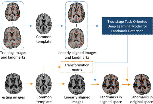
Illustration of the proposed two-stage task-oriented deep learning (T²DL) framework for landmark detection with medical images.

Figure 2 illustrates the architecture of the proposed T²DL model, where we learn a two-stage deep CNN model in a cascaded manner. Specifically, we first train a patch based CNN regression model to describe the non-linear mapping between local image patches and their 3D displacements to the target landmarks, using millions of image patches as training samples. In the second stage, we develop another CNN model by adding extra layers to an FCN model, which shares the same architecture and network weights as the CNN used in the first stage. In particular, the CNN model in the second stage can predict the coordinates of multiple landmarks jointly, with an entire image as input and the landmark coordinates as output. In this way, both local information (i.e., the inherent associations between image patches and their displacements to landmarks) and global information (i.e., the association among image patches) can be integrated into the learning process via CNN in the first and second stages, respectively. Our method achieves a mean error of 2.96 mm in brain landmark detection using MR data (with 1200 landmarks and 700 subjects), and a mean error of 3.34 mm in prostate landmark detection using CT data (with 7 landmarks and 73 subjects). Also, our method requires only approximately 1 second to detect thousands of landmarks simultaneously.

Fig. 2.

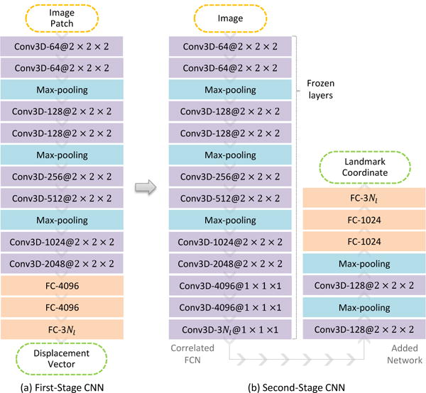
Illustration of our proposed two-stage task-oriented deep neural network model, where Conv3D denotes 3D convolutional layer and FC means fully connected layer. The activation function is not shown for brevity.

II. Related Work

In the literature, extensive methods are proposed for facial landmark detection and anatomical landmark detection. In general, these methods can be roughly divided into three categories, including 1) keypoint based methods [11], 2) atlas based methods [12], and 3) learning based methods [13], [14], [15], [16], [17], [18]. Specifically, in keypoint based methods, points of interest (such as symmetry maxima, and Harris corners) detectors are adopted to identify candidates for individual model landmarks, and perform discrete optimization of a graph matching problem to obtain the final localization of landmarks. However, these methods cannot detect landmarks that are not located in salient corners or boundaries. Atlas based methods usually require an atlas with pre-defined landmarks. The landmarks for a testing image can be directly transferred from corresponding landmarks in the atlas image by using the estimated deformation field via registration. The main problem of these atlas based methods is that they largely rely on the accuracy of cross-subject registration. Although multi-atlas registration can improve the robustness and accuracy, it is very time intensive to perform multiple registrations for each testing subject. Different from the former two sets of methods, learning based methods utilize learning algorithms in machine learning domain for landmark detection and have demonstrated superiority in anatomical landmark detection for medical images [6], [19].

Many learning based landmark detection methods for medical images aim to learn classification/regression models by using image patches as training samples. Currently, there are a large number of classification based methods for localizing anatomical landmarks or organs [20], [19]. In these methods, voxels near a specific landmark are regarded as positive samples and the rest are used as negative ones. For each voxel, a cubic patch is extracted (usually described by handcraft features [21], [22], [23], [24]), and then a patch-wise binary classifier [25], [26], [27], [28] is learned to localize anatomical landmarks. As another typical learning based framework in landmark detection, regression based methods focus on learning the non-linear relationship between a local patch and its 3D displacements to a target landmark via a regression model (e.g., random forest, and CNN). That is, each local patch can be used to estimate a potential landmark position. Given plenty of image patches, the optimal landmark position can be estimated by assembling the predictions of a tremendous amount of image patches, e.g., via a majority voting strategy [15], [13]. Therefore, context information from nearby patches can be utilized to localize landmarks. Recently, regression based methods have demonstrated their superiority in different medical applications [29], [14], [15], [30], [18]. Although patch based approaches can partly alleviate the problem of limited medical data (by using millions or even billions of patches as training samples), it is generally time-consuming to simultaneously predict landmarks from a massive amount of 3D image patches. Also, patch based methods can only model local information (i.e., relationships between patches and their displacements to landmarks), while global information (e.g., the correlations among patches) is ignored in the learning process.

A few previous studies have adopted an end-to-end learning strategy for anatomical landmark detection, through which the relationship among landmarks and patches can be captured. In these methods, landmark detection is often formulated as a regression problem [4], [10], with the goal of learning a non-linear mapping between an input image and landmark coordinates. In this way, the landmark position can be directly estimated via deep learning models (e.g., CNN). Besides, FCN based methods achieve impressive performance in object detection and landmark detection [31], [32], [33], [34]. Recently, Payer et al. [6] have tested several FCN architectures for detecting anatomical landmarks with limited medical imaging data, where each landmark position is marked as a heat map corresponding to the original image. Reasonable detection performance is obtained, which helps illustrate the effectiveness of FCN in detecting anatomical landmarks. However, due to the limited training data, very shallow networks were used in the experiment, which could not entirely capture the discriminative information in the medical images. Also, it is almost impossible to simultaneously detect large-scale landmarks in an end-to-end manner, since each landmark corresponds to an output of a 3D heat map and thus the existing GPU memory cannot deal with thousands of 3D output maps together. In contrast, if multiple landmarks are detected separately, it is cumbersome to train many models and also the underlying correlations among landmarks will be ignored.

Our proposed two-stage task-oriented deep learning (T²DL) method is inspired by both patch based and end-to-end learning methods. First, to overcome the problem of limited training data, we propose a patch based CNN regression model in the first stage, by using millions of image patches as training samples. Then, we develop another CNN model in the second stage to jointly detect large-scale landmarks in an end-to-end manner, where the global structural information of images can be naturally captured and integrated into the learning process.

III. Method

In this study, we attempt to deal with two challenging problems in detecting anatomical landmarks with medical imaging data, i.e., 1) limited training data and 2) large-scale landmarks. As shown in Fig. 2, we propose a two-stage task-oriented deep learning (T²DL) method, where each network has its specific task. Specifically, the task of the first-stage CNN model is to describe the inherent associations between local image patches and their 3D displacements to the target landmarks, with millions of image patches as the input. The task of the second-stage CNN model is to estimate the landmark coordinates by considering correlations among image patches, with the entire image as the input. The following sub-sections describe the architecture of the proposed T²DL method in detail.

A. First Stage: Modeling Associations between Image Patches and Displacements to Landmarks

We first develop a patch based CNN regression model by using local image patches rather than the entire images, as the training samples. However, the conventional patch based methods usually directly estimate the class label (i.e., a certain landmark) of a voxel from local patches, where the context information of the image patches is not considered. In this study, we propose to estimate the displacements of an image patch to multiple landmarks for implicitly modeling the context information. Given a 3D image patch, our goal is to learn a non-linear mapping to predict its 3D displacements to multiple landmarks. The conventional patch based landmark detection methods build the mapping using random forest regression models [14], [13], and usually require pre-defined appearance features to represent image patches. Without using any pre-defined features, we adopt a patch based regression model using CNN. As shown in Fig. 2(a), the first-stage CNN model consists of 8 convolutional layers, 3 max-pooling layers, and 3 fully connected layers. In the training stage, we sample a tremendous amount of image patches to learn a deep CNN model. In this way, each local patch can then be used as a training sample to estimate its 3D displacements to multiple landmarks.

Due to variations of shape across subjects, the estimation of displacements for faraway landmarks from local image patches are often inaccurate [13]. Thus, we propose to adopt a weighted mean squared error as a loss function in the first-stage CNN model, by assigning lower weights to the displacements for faraway landmarks from image patches. Specifically, we define the 3D displacement from a local image patch to the i-th target landmark as ${\stackrel{\sim }{d}}_i={[\mathrm{\Delta }{x}_i,\mathrm{\Delta }{y}_i,\mathrm{\Delta }{z}_i]}^T$, where Δx_i, Δy_i, and Δz_i denote the displacements between the specific patch to the i-th landmark w.r.t. x, y, and z axes, respectively. Suppose ${\stackrel{\sim }{d}}_i^g$ is the ground-truth displacement and ${\stackrel{\sim }{d}}_i^p$ is the predicted displacement. Our proposed weighted mean squared loss function is defined as

$$\mathit{Loss}=\frac{1}{N_l}{\displaystyle \sum _{i=1}^{N_l}{w}_i\Vert {\stackrel{\sim }{d}}_i^g-{\stackrel{\sim }{d}}_i^p{\Vert }_2},$$ (1)

where $w_i=e^{-\frac{\Vert {\stackrel{\sim }{d}}_i^g\Vert }{\alpha }}$, α is a scaling coefficient, and N_l is the total number of landmarks. By using the weighted loss function, patches are expected to contribute more to their nearby landmarks, but less to those faraway landmarks. In this way, we can reduce instability between local image patches and their corresponding faraway landmarks, which could potentially lead to robust performance in estimating displacements.

Intuitively, given a testing image, we first sample lots of local image patches, and then compute their displacements to landmarks via the first-stage CNN model. Since each patch can cast a vote to multiple landmarks, the final landmark positions for the testing image can be estimated by using the mean positions or the majority-voted positions based on those local patches. However, it is generally very time-consuming to predict displacements for a tremendous amount of 3D image patches, even the estimation of displacement from each image patch is fast. To this end, we further propose to integrate the patch based CNN model into a fully convolutional network (FCN) for jointly predicting displacements (to multiple landmarks) of those grid-sampled patches. As shown in Fig. 3, grid-sampled patches denote local image patches that are sampled from an entire image in a grid defined by a specific pooling strategy in FCN, with details given below.

Fig. 3.

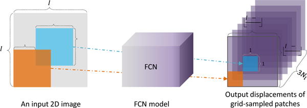
2D illustration of the fully convolutional network (FCN). Given an input 2D image, FCN first extracts multiple local image patches in a grid with the step size of n_p via the first max-pooling operation (with the kernel size of k × k). Here, we denote the orange and blue blocks as two p × p patches. The estimated displacements of these two grid-sampled patches are the two 1 × 1 × 3N_l elements in the outputs of FCN for one specific landmark.

B. Second Stage: Modeling Correlations among Image Patches

Coincidentally, if the neural network is carefully designed, the first-stage CNN model can be perfectly correlated to an FCN model that treats the entire image as input and the displacements of grid-sampled patches as output. Specifically, as shown in Fig. 2, the difference between the first-stage CNN and the FCN in the second stage is that the last three fully connected layers in CNN are replaced by three convolutional layers with the kernel size of 1 × 1 × 1 in the FCN. We can directly apply the learned network weights of the first-stage CNN to its correlated FCN model in the second stage. Given an input image, the displacements of grid-sampled patches to multiple landmarks can be predicted jointly via FCN.

As shown in Fig. 3, the output size of FCN is determined by both patch size and pooling size. Suppose the input image size is I_x × I_y × I_z, the patch size is p × p × p, and we have a total of n_p pooling operations with the kernel size of k × k × k in the network. In FCN, we implement a valid filtering strategy and non-overlapping pooling. As shown in Fig. 2, there are 3 max-pooling procedures with the kernel size of 2 × 2 × 2, and hence the down-sampling rate is $\frac{1}{2^3}$. Given N_l landmarks, the output size of FCN for an input image is defined as $\lfloor \frac{I_x-p}{n_p^k}\rfloor \times \lfloor \frac{I_y-p}{n_p^k}\rfloor \times \lfloor \frac{I_z-p}{n_p^k}\rfloor \times 3N_l$, with ⌊·⌋ denoting the floor operator.

It is intuitive to compute the optimal landmark positions by assembling the predictions of a tremendous amount of grid-sampled patches. Similar to the strategy we developed for the weighted loss in the first stage, we adopt a weighted voting strategy to obtain the optimized landmark positions. We can assign large voting weights for image patches near to the landmarks (i.e., defined by their estimated displacements), and small weights for those faraway image patches. However, as a consequence, the underlying correlations among local image patches are completely ignored. For instance, the nearby image patches may contribute similarly to a specific landmark. Therefore, we propose to add more layers to the above-mentioned FCN model, to take advante of the association of patches.

As shown in Fig. 2(b), in the added network, the first 2 convolutional layers are used to associate those neighboring displacements of grid-sampled patches, and thus the outputs of those neighboring patches are integrated together to generate strong estimation. Also, the max-pooling operation can potentially decrease the negative impact of those inaccurate predictions. Next, we add other 3 fully connected layers to further build the connections among patches and landmarks. Importantly, the landmark coordinates can be regarded as the output of the added network. That is, the second-stage CNN model is a full end-to-end model, consisting of an FCN and an added network, where the entire image and landmark coordinates are treated as input and output, respectively.

C. Implementations

In the training stage, we first sample a tremendous amount of 3D image patches with a fixed size. Since there may exist large regions with uniform tissue in the medical images, it is not reasonable to adopt random sampling strategy to sample patches, since this could lead to a large number of uninformative image patches. To balance the proportions of uninformative (or less informative) and informative image patches, we sample image patches according to the probabilities calculated by local entropies from the entire image. Specifically, we first calculate the local entropy $E(\widehat{\eta })$ for a region around each image patch $\widehat{\eta }$, with the larger value of $E(\widehat{\eta })$ denoting that the voxel $\widehat{\eta }$ being more informative. Then, we sample the image patch $\widehat{\eta }$ with the probability of $\mathcal{P}(\widehat{\eta })=e^{-\frac{\beta }{E(\widehat{\eta })}}$, where β is a coefficient used to adjust the sampling probability.

Using image patches as input samples, we train the first-stage CNN regression model with the task of estimating 3D displacements to all landmarks. These 3D displacements are stretched and concatenated as multivariate targets of the regression model. We design our CNN model to guarantee that the output size of the last convolutional layer (before fully connected layers) is 1 × 1 × 1 × 3N_l. Therefore, the network weights of the patch based CNN model in the first stage can be directly assigned to the correlated FCN model in the second stage. In the second stage, by freezing the FCN network, we only learn the network weights of the added network. Since those accurately predicted displacements (i.e., outputs of FCN) make the detection problem much easier and the added network is not very deep, a robust landmark detection model can be trained even with limited training images. In addition, the full implementation of the proposed CNN model is based on Tensorflow [35], and the computer we used in the experiments contains a single GPU (i.e., NVIDIA GTX TITAN 12GB).

IV. Experiments

A. Datasets

We evaluate our proposed T²DL method on two datasets with 3D brain MR data and 3D prostate CT data, respectively. In the brain MR dataset, we have two individual subsets that contain 400 subjects with 1.5 T T1-weighted MR images (denoted as ${\mathcal{D}}_1$) and 300 subjects with 3.0 T T1-weighted MR images (denoted as ${\mathcal{D}}_2$), respectively. The size of images in ${\mathcal{D}}_1$ and ${\mathcal{D}}_2$ is 256 × 256 × 256, and the spatial resolution is 1 × 1 × 1 mm³. Exemplar MR images from ${\mathcal{D}}_1$ and ${\mathcal{D}}_2$ can be found in Fig. S3 in the Supplementary Materials. For this dataset, we annotate the ground-truth landmarks in MR images through a two-step process. Specifically, in the first step, we adopt a group comparison algorithm proposed in [36] to generate a large number (~ 1700) of anatomical landmarks. This algorithm aims to identify the landmarks that have statistically significant group differences between Alzheimer’s disease patients and normal control subjects in local brain structures [36]. In the second step, we ask three experts to annotate those unreliable landmarks. The criterion here is that, if one landmark is annotated as unreliable by at least one expert, this landmark will be deleted from the landmark pool. In this way, we obtain 1200 anatomical landmarks defined. Typical landmarks are shown in Fig. 4 (a). For this dataset, we perform three groups of experiments to evaluate the robustness of our method. To be specific, in the first group (denoted as ${\mathbb{G}}_1$), we use MR images in ${\mathcal{D}}_1$ and ${\mathcal{D}}_2$ as training and testing data, respectively. In the second group (denoted as ${\mathbb{G}}_2$), we treat ${\mathcal{D}}_2$ and ${\mathcal{D}}_1$ as the training set and the testing set, respectively. In the third group (denoted as ${\mathbb{G}}_3$), we randomly select 200 images from ${\mathcal{D}}_1$ and 150 images from ${\mathcal{D}}_2$ to construct the training set, and the remaining images in ${\mathcal{D}}_1$ and ${\mathcal{D}}_2$ are used as the testing data.

Fig. 4.

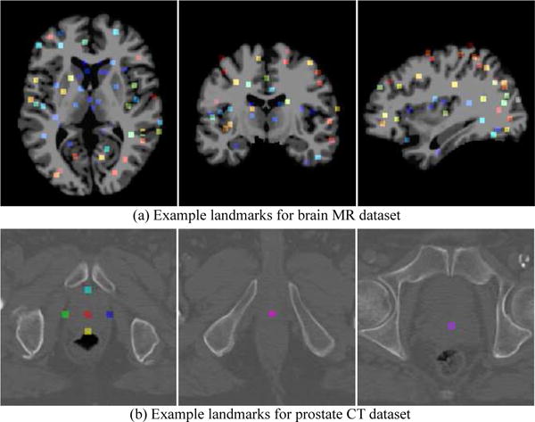
Example anatomical landmarks on (a) brain MR dataset, and (b) prostate CT dataset.

In the prostate CT dataset, we have CT images from 73 subjects. The size of images in this dataset is 512×512×61 (or 512×512×81), with the spatial resolution of 0.938×0.938× 3 mm³. For this dataset, we have 7 prostate anatomical landmarks manually annotated by two experts. These landmarks include seven key points in the prostate, including prostate center, right lateral point, left lateral point, posterior point, anterior point, base center, and apex center. Typical landmarks are shown in Fig. 4 (b). A five-fold cross-validation strategy is adopted for this dataset. Specifically, all subjects are randomly divided into five roughly equal subsets, and subjects in one subset are used for testing, while subjects in the remaining four subsets are used for training.

B. Experimental Settings

For those MR and CT images, we first perform linear registration to one fixed image (i.e., randomly selected from the corresponding dataset). To speed up the linear registration, we down-sample images to perform linear registration, and then rectify the transformation matrix to the original image space. Considering the GPU memory, we resize the original image and crop it by removing the background. Since all images are linearly aligned, the images can be cropped using the same strategy. Specifically, for brain MR images, we crop the original images into the size of 152 × 186 × 144. While, for prostate CT images, we resized them to have the spatial resolution of 0.938 × 0.938 × 0.938 mm³ and then crop them into the size of 140 × 140 × 140 mm³. Since MR and CT images have different sizes and landmark numbers, the added network in the second-stage CNN model (see Fig. 2(b)) is slightly different for brain MR data and prostate CT data. Denoting N_l as the number of landmarks, the last three fully connected layers are of (1024, 1024, 3N_l) dimensions for brain landmark detection model, and of (512, 256, 3N_l) dimensions for prostate landmark detection model. The parameters α in the weighted loss function and β in patch sampling are empirically set as 0.6 and 15, respectively. In T²DL, we generally adopt ReLU activation function for both convolutional layers and fully connected layers. In the last layers of the first-stage and the second-stage CNN models, we use tanh activation function. The max-pooling is performed in a 2×2×2 window, and the patch size is empirically set as 38 × 38 × 38.

C. Competing Methods

We first compare T²DL with two baseline methods, including 1) multi-atlas (MA) based method using non-linear registration [37], 2) random forest (RF) regression [38], [13]. We further compare our method with two state-of-the-art approaches, i.e., 3)shallow convolutional neural network (Shallow-Net), and 4) U-Net [6]. Besides, we compare the proposed method with a patch based CNN model, which is a variant of T²DL (called First-Stage-Only). We now briefly introduce these methods as follows.

1. Multi-Atlas (MA) based method with non-linear registration [37]. In MA, we first randomly select 20 images from the training set as atlases to perform deformable registration. For a particular landmark, we map this landmark from the corresponding positions in the non-linearly aligned atlases to each testing image, and hence can obtain 20 warped landmark positions on each testing image. We then average them to obtain the final landmark location on the testing image.

2. Random forest (RF) regression method based on image patches [38], [13]. In RF, we learn a non-linear mapping between a local patch and its displacement to a target landmark via a random forest regression model. Specifically, we adopt a coarse-to-fine strategy to train landmark detector for each landmark individually. During the feature extraction stage, we extract Haar-like features for each patch with the size of 32 × 32 × 32. For the random forest construction, we adopt 20 trees and the depth of each tree as 25. We adopt the majority voting strategy to obtain the final landmark locations.

3. Shallow convolutional neural network (Shallow-Net) [39], which detects landmarks in an end-to-end manner. In Shallow-Net, we train a shallow regression network to predict landmark coordinates using an entire image as input. The architecture of Shallow-Net consists of 3 convolutional layers with the kernel size of 3×3×3 and 3 fully connected layers, and each convolutional layer is followed by a 3×3×3 max-pooling layer. The element numbers in the three fully connected layers are (512, 1024, N_l) and (256, 128, N_l) for brain landmark and prostate landmark detection models, respectively.

4. U-Net [40], which is a typical fully convolutional network. Following [6], we adopt heat maps of landmarks as target outputs, using the same parameters as those in [6]. For each landmark, we generate a heat map using a Gaussian filtering with the standard derivation of 3 mm. We use 3 × 3 × 3 kernels for convolution, while down-sampling and up-sampling are performed in a 3×3×3 window. ReLU activation function and average pooling are adopted in U-Net.

5. First-stage deep learning (First-Stage-Only) model with image patches as input, which is a variant of our T²DL method. As shown in Fig. 2(a), First-Stage-Only denotes the first-stage CNN model in T²DL, where landmarks are detected by weighted majority voting on predicted displacements of patches to landmarks.

D. Landmark Detection Results

We first report landmark detection errors achieved by different methods on both brain MR and prostate CT datasets in Table I. Considering the computational cost and limited memory, it is difficult for RF and U-Net to detect large-scale landmarks in the brain. Thus, besides those original 1200 brain landmarks, we also randomly select 10 landmarks from the brain MR dataset, and perform an additional experiment by comparing the proposed methods with RF and U-Net on this subset of brain landmarks. Thus, in Table I, we show the landmark detection results of three tasks, including 1) detection of 1200 brain landmarks on the brain MR image dataset (Brain-1200), 2) detection of 10 brain landmarks on the brain MR image dataset (Brain-10), and 3) detection of 7 prostate landmarks on the prostate CT image dataset (Prostate-7). Note that, in the following text, without additional explanation, the brain landmark detection task refers to the detection for those original 1200 landmarks on the brain MR imaging dataset throughout this paper.

TABLE I.

Landmark detection errors on brain dataset and prostate dataset (mm)

Methods	Brain-1200			Brain-10			Prostate-7
	${\mathbb{G}}_1$	${\mathbb{G}}_2$	${\mathbb{G}}_3$	${\mathbb{G}}_1$	${\mathbb{G}}_2$	${\mathbb{G}}_3$
MA	3.05 ± 1.69	3.08 ± 1.72	3.07 ± 1.71	2.98 ± 1.67	3.03 ± 1.68	3.01 ± 1.66	5.18 ± 3.27
RF	–	–	–	3.35 ± 2.17	3.37 ± 2.30	3.31 ± 2.19	4.75 ± 2.98
Shallow-Net	4.43 ± 2.76	4.35 ± 2.72	4.20 ± 2.55	4.28 ± 2.90	4.25 ± 2.92	4.19 ± 2.78	6.70 ± 3.01
U-Net	–	–	–	3.62 ± 2.46	3.70 ± 2.51	3.55 ± 2.50	4.68 ± 2.40
First-Stage-Only	3.39 ± 1.98	3.37 ± 2.06	3.29 ± 1.85	3.30 ± 1.97	3.35 ± 2.14	3.25 ± 1.87	4.36 ± 2.35
T2DL (Proposed)	2.96 ± 1.59	2.98 ± 1.63	2.94 ± 1.58	2.86 ± 1.53	2.90 ± 1.61	2.82 ± 1.52	3.34 ± 2.55

From Table I, we can make the following observations. First, the proposed T²DL method achieves much lower detection errors on both datasets, compared with other four methods. For instance, for the prostate landmarks, the detection error obtained by T²DL is 3.34 mm, which is lower than the other four methods by at least 1.02 mm. Second, one can observe that Shallow-Net achieves a relatively poor landmark detection performance on three tasks. This could be due to its shallow architecture induced by limited training data. With a similar shallow architecture, U-Net outperforms Shallow-Net to a large extent, which can be attributed to the use of heat map. Third, RF achieves comparable results with our First-Stage-Only method, since they are patch based methods and share similar protocol to localize landmarks. Fourth, since First-Stage-Only uses just the first-stage FNN model of T²DL, its performance is much worse than T²DL in both brain landmark and prostate landmark detection tasks. A possible reason is that, besides local information (i.e., the associations between patches and landmarks) described by First-Stage-Only, T²DL further considers global information (i.e., the association among image patches) of the entire image via the added network. Fifth, MA achieves relatively good performance on detecting brain landmarks and poor performance on detecting prostate landmarks. The reason could be that it is easy to perform the nonlinear registration among brain MR images but difficult for prostate CT images. Moreover, it is time-consuming for nonlinear registration, especially for multiple atlases. In particular, our T²DL generally obtains better results compared with U-Net which performs the task of landmark detection via heat map regression. Actually, the heat map regression here is more like a classification task. That is, it directly estimates the probability of a voxel being a landmark based on structural information of landmark regions only, and does not utilize the contextual information of the whole image. In contrast, our method can model the contextual information of landmarks, by simultaneously estimating the displacements of a voxel to multiple landmarks. This could partly explain why our method is superior to U-Net.

We then show the cumulative distributions of landmark detection errors achieved by different methods in Fig. 5. From the figure, we can observe that most landmarks can be detected within a low error range using our two-stage task-oriented network. Also, the superiority of our proposed T²DL method over the competing methods is prominent in the task of prostate landmark detection. Importantly, it only requires approximately 1 second (with single NVIDIA GTX TITAN 12GB) for T²DL to complete the detection process of detecting multiple (e.g., 1200) landmarks for one image, which can be considered real-time. The underlying reason for the low computation time is the use of fully convolutional layers in the proposed second-stage CNN. Due to the overlapping regions of local image patches, the computation is highly amortized over the overlapping regions of those patches. Thus, both the feedforward computation and the backpropagation in the proposed second-stage CNN are much more efficient when computed layer-by-layer over the entire image instead of independently patch-by-patch.

Fig. 5.

Cumulative distribution of landmark detection errors achieved by different methods on (a) brain MR dataset with 1200 landmarks (Brain-1200), (b) brain MR dataset with 10 landmarks (Brain-10), and (c) prostate CT imaging dataset with 7 landmarks (Prostate-7).

Qualitatively, we also illustrate the landmark detection results achieved by our T²DL method in Fig. 6. For brain landmarks, we illustrate the 3D rendering of our sampled 10 landmarks in 3D brain MR images, since it is unclear to visualize too many landmarks in a single slice or a 3D rendering volume. The 3D rendering videos are provided in the Supplementary Materials for clear visualization. As shown in Fig. 6 (a), most of our detected landmarks (i.e., red points) are overlapping with or very close to the ground-truth landmarks (i.e., green points). For prostate landmarks, we show example landmarks in one slice in Fig. 6 (b). Similar to the results of brain landmark detection, the prostate landmarks detected by T²DL are very close to the ground-truth landmarks.

Fig. 6.

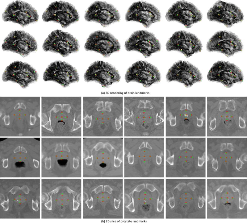
Illustration of landmark detection results by the proposed T²DL method in tasks of (a) brain landmark detection and (b) prostate landmark detection. Here, red points denote our detected landmarks via T²DL, while green points represent the ground-truth landmarks.

We further report the change of loss function values achieved by the proposed T²DL model training with entire images, as shown in Fig. 7. This figure indicates almost no over-fitting issue in T²DL, even if limited training subjects are used. Specifically, in brain MRI dataset with 400 subjects and 1200 landmarks, the loss on the validation set is very similar to that on the training set. A similar trend can be found from the results on the prostate CT dataset. That is, the losses of both training set and validation set are very similar, indicating almost no over-fitting issue in our proposed T²DL model. In addition, we perform an experiment to simply train the second-stage CNN without using the pre-training strategy. However, we found that the CNN model has the over-fitting problem, since the validation error is much larger than the training error. One possible reason could be that we have only a very limited number (i.e., hundreds) of training images. This further demonstrates the effectiveness of the proposed first-stage pre-training strategy.

Fig. 7.

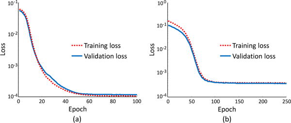
Change of loss function values concerning different epoch achieved by the proposed T²DL model on (a) brain MR dataset (Brain-1200) and (b) prostate CT dataset.

V. Discussion

In this section, we first flesh out the difference between T²DL and conventional methods, and then analyze the influences of parameters. We also elaborate several limitations of our method. In the Supplementary Materials, we further investigate the influences of interpolation algorithm, the distance among landmarks, and our two-stage learning strategy.

A. Comparison with Conventional Methods

There are at least two differences between our T²DL method and previous patch based approaches. First, in contrast to the conventional patch based learning methods that often rely on specific decision-making strategies (e.g., majority voting), our T²DL method can learn to design the suitable features and integration strategies to jointly detect multiple landmarks in an end-to-end manner. Second, T²DL can model both local and global information of images via a two-stage learning model, while the conventional methods often ignore global correlations among image patches. Experimental results in Table I demonstrate that T²DL outperforms patch based methods (i.e., RF, and First-Stage-Only) that consider only local information. This implies that integrating both local and global information into the learning model may help promote the performance of landmark detection.

Compared with the conventional end-to-end learning methods, the prominent advantage of T²DL is that it can partly solve the problem of limited training data in the medical imaging applications. Our strategy is to train a CNN model using 3D image patches, rather than the entire image in the first stage. In this way, we can learn a very deep CNN model to precisely model the inherent associations between image patches and their displacements to multiple landmarks, by using millions of local patches as the input. In contrast, the conventional end-to-end learning methods (e.g., Shallow-Net, and U-Net) usually have very shallow architecture, because of using limited training data. Since shallow networks are not powerful enough to capture discriminative information of medical images with complex local structures, they cannot achieve good performance in landmark detection (see Table I and Fig. 5). Also, T²DL can jointly detect large-scale landmarks in real time, while the conventional FCN models (e.g., U-Net) cannot simultaneously deal with thousands of 3D output maps (corresponding to thousands of landmarks) which are very high dimensional.

B. Influence of Training Subject Number

We investigate the influence of the number of training subjects on landmark detection performance, with results shown in Fig. 8. In brain landmark detection, we randomly select training subjects from D_1 for model training, and then validate the learned model on D_2. In prostate landmark detection, we randomly select 13 subjects as testing data, while training subjects are randomly selected from the rest. As shown in Fig. 8, as an end-to-end learning method, T²DL achieves quite stable performance with the different number of training subjects, while the landmark detection errors achieved by Shallow-Net and U-Net decrease a lot with the increase of training subject number. As patch based methods, RF and First-Stage-Only are not very sensitive to the number of training subjects. The possible reason could be that there is no severe deformation in the linearly aligned images, and thus patch based methods (that rely on thousands of local image patches, rather than entire images of subjects) are relatively robust to the number of training subjects. Compared with First-Stage-Only, T²DL is more sensitive to the number of training subjects. Also, as shown in Fig. 8(a), using 50 training subjects, First-Stage-Only achieves an error of 3.49, which is slightly better than T²DL on the brain MR dataset. Thus, if there are very few training subjects and large-scale landmarks in a real application, the use of First-Stage-Only, rather than T²DL, could be a better solution. On the other hand, using only 10 training subjects, T²DL achieves appealing performance on the prostate CT dataset with only 7 landmarks. In contrast, it requires more training data for T²DL to detect large-scale (1200) brain landmarks, since more network weights need to be learned in the second-stage CNN model of T²DL.

Fig. 8.

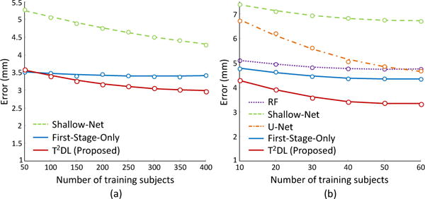
Landmark detection errors by different methods with respect to the different number of training subjects on (a) brain MR dataset (Brain-1200) and (b) prostate CT dataset.

C. Influence of Weighted Loss

We further evaluate the influence of the proposed weighted loss function (Eq. 1) on the performance of the proposed methods (i.e., T²DL and First-Stage-Only). In the experiments, we compare the weighted loss function with the conventional loss function (without weighting strategy). The experimental results are reported in Fig. 9. It can be seen that the methods using the proposed weighted loss function consistently achieve better performance in both brain landmark and prostate landmark detection tasks. Specifically, the detection errors by T²DL with the proposed weighted loss function are 2.96 mm and 3.34 mm on the brain and prostate datasets, respectively, while the detection errors by the conventional loss are only 3.26 mm and 3.45 mm, respectively. Similarly, First-Stage-Only with the proposed weighted loss can achieve much lower detection errors than that using conventional loss. This suggests that using the weighted loss function can further boost landmark detection performance, where local image patches are encouraged to contribute more to the nearby landmarks and less to the faraway ones. The main reason is that such strategy can help reduce the variance of displacements (between local image patches and landmarks) caused by shape variation across subjects.

Fig. 9.

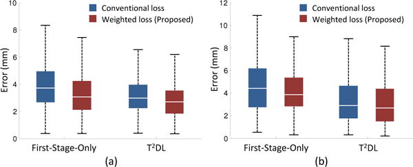
Landmark detection errors achieved by First-Stage-Only and T²DL using different loss functions on (a) brain MR dataset (Brain-1200) and (b) prostate CT dataset.

D. Influence of Patch Size

In all above-mentioned experiments, we adopt a fixed patch size (i.e., 38×38×38) for the proposed T²DL and First-Stage-Only methods. Here, we investigate the influence of patch size on the performance of T²DL and First-Stage-Only in detecting both brain landmarks and prostate landmarks. Specifically, we vary the patch size in a range of [18 × 18 × 18, 28 × 28 × 28, 38 × 38 × 38, 48 × 48 × 48], and record the corresponding results in Fig. 10. Note that, given different input patch size, the network architecture of our model is slightly changed to guarantee that output size of the last convolutional layer in First-Stage-Only is 1 × 1 × 1 × 3N_l.

Fig. 10.

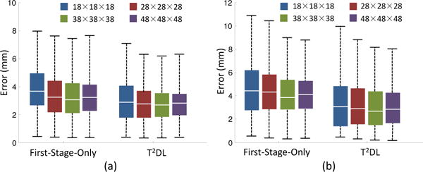
Influence of local image patch size on the performances of First-Stage-Only and T²DL when used in (a) brain MR dataset (Brain-1200) and (b) prostate CT dataset.

As shown in Fig. 10, the landmark detection errors achieved by T²DL fluctuate in a small range. For instance, on the brain MR dataset, T²DL produces an error of 3.21 mm using the patch size of 48 × 48 × 48, and an error of 3.12 mm with the patch size of 28 × 28 × 28. We can observe a similar trend for our First-Stage-Only method on those two datasets. These results imply that our proposed T²DL and First-Stage-Only methods are not very sensitive to the patch size. Also, Fig. 10 indicates that, using large patch size (e.g., 48 × 48 × 48) often leads to the smaller standard deviation, compared with that using small patch size (e.g., 18 × 18 × 18). It implies that the use of large patch size often leads to relatively more robust, but not always very accurate landmark detection results. In addition, our method does not achieve good results using a small patch size (i.e., 18 × 18 × 18) on two datasets. One possible reason could be that a small patch could not entirely capture the region’s discriminative structural information by allowing the network to see only little context, while the local structure (captured by a small patch) of a particular region (e.g., a small cortical region) could be ambiguous because of the variation among subjects. In contrast, a relatively large patch can not only model the structure of this small region, but also the context information of this region. For brain MR and prostate CT images used in this study, it is reasonable to adopt patch size between 28 × 28 × 28 and 38 × 38 × 38.

E. Influence of Down-sampling Rate

We also investigate the influence of down-sampling rate on the performance of our proposed First-Stage-Only and T²DL methods, where the down-sampling rate is determined by both the number and the kernel size of pooling procedures in CNN model. In the experiments, we vary the number of max-pooling process (with the kernel size of 2 × 2 × 2) in the range of [2, 3, 4], and record the corresponding results achieved by First-Stage-Only and T²DL in Fig. 11.

Fig. 11.

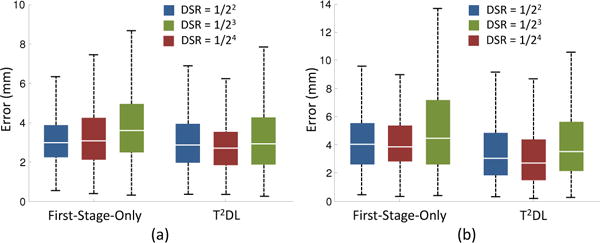
Influence of down-sampling rate on the performances of First-Stage-Only and T²DL when used in (a) brain MR dataset (Brain-1200) and (b) prostate CT dataset. DSR: Down-sampling rate.

It can be observed from Fig. 11 that both First-Stage-Only and T²DL achieve the worst performances when using the down-sampling rate of $\frac{1}{2^4}$, in both brain landmark and prostate landmark detection tasks. In particular, First-Stage-Only with a down-sampling rate of $\frac{1}{2^4}$ achieves an error of 5.29 mm in prostate landmark detection, which is higher than using down-sampling rate of $\frac{1}{2^2}$ and $\frac{1}{2^3}$ by at least 0.93 mm. The main reason is that, if we use a high down-sampling rate, the outputs of First-Stage-Only are of very low dimension. Hence, the outputs of FCN are displacements for very few sampled patches, leading to unstable estimations of landmark positions. If we adopt a low down-sampling rate (e.g., $\frac{1}{2^2}$), the outputs of FCN will be high-dimensional, which could lead to an over-fitting problem for the second-stage CNN with limited data.

F. Limitations and Future Work

Although our proposed T²DL method shows significant improvement in terms of landmark detection accuracy over conventional patch based and end-to-end learning methods, several technical issues need to be considered in the future. First, we empirically adopt a fixed patch size (i.e., 38×38×38) to train a CNN model in the first stage of T²DL. Multiscale patch size could be more reasonable for patch based CNN regression model, since the structural changes caused by diseases could vary highly across different landmark locations. Second, in this study, we treat all landmarks equally in both brain dataset and the prostate dataset. Actually, different landmarks may have different importance in real applications, and thus should be assigned different weights in the learning model for further boosting the learning performance. Third, there are only 7 anatomical landmarks annotated by experts for CT images in the prostate dataset. As one of our future work, we will ask experts to annotate more landmarks for this dataset. Furthermore, the large-scale 1200 brain landmarks are defined using group comparison for the purpose of brain disease diagnosis [36]. Specifically, as we did in our previous work [36], we can extract morphological features from each landmark location. Since these landmarks are distributed in the whole brain, we can extract morphological features based on landmarks for computer-aided disease diagnosis. Also, we can locate informative image patches in MRI based on these landmarks, and then automatically learn discriminative features (e.g., via deep convolutional neural network) from MR image patches for subsequent tasks (e.g., classification, regression, and segmentation). However, there may be missing or redundant landmarks for brain MR images, which is not considered in this study. A reasonable solution is to perform manual correction to add more discriminative landmarks, or to remove redundant landmarks based on expert knowledge.

VI. Conclusion

We propose a two-stage task-oriented deep learning (T²DL) method for anatomical landmark detection with limited medical imaging data. Specifically, the task in the first stage is to capture inherent associations between local image patches and their corresponding displacements to multiple landmarks via a patch based CNN model. In the second stage, we focus on predicting landmark coordinates directly from the input image via another CNN model in an end-to-end manner, where the correlations among image patches can be captured explicitly. The proposed T²DL model can be effectively trained in a local-to-global task-oriented manner, and multiple landmarks can be jointly detected in real time. Our results on two datasets with limited medical imaging data show that our method outperforms many state-of-the-art methods in landmark detection. The proposed method may be applied to various other applications, such as image registration, image segmentation, and neurodegenerative disease diagnosis.

Biographies

Jun Zhang was born in Shaanxi province, China. He received the B.S. degree in 2009 and Ph.D. degree in 2014 from Xidian University, Xi’an, China. His research interests include image processing, machine learning, pattern reognition, and medical image analysis.

Mingxia Liu received the B.S. and M.S. degrees from Shandong Normal University, Shandong, China, in 2003 and 2006, respectively, and the Ph.D. degree from Nanjing University of Aeronautics and Astronautics, Nanjing, China, in 2015. Her current research interests include neuroimaging analysis, machine learning, pattern recognition, and data mining.

Dinggang Shen is Jeffrey Houpt Distinguished Investigator, and a Professor of Radiology, Biomedical Research Imaging Center (BRIC), Computer Science, and Biomedical Engineering in the University of North Carolina at Chapel Hill (UNC-CH). He is currently directing the Center for Image Analysis and Informatics, the Image Display, Enhancement, and Analysis (IDEA) Lab in the Department of Radiology, and also the medical image analysis core in the BRIC. He was a tenure-track assistant professor in the University of Pennsylvanian (UPenn), and a faculty member in the Johns Hopkins University. Dr. Shenbs research interests include medical image analysis, computer vision, and pattern recognition. He has published more than 700 papers in the international journals and conference proceedings. He serves as an editorial board member for eight international journals. He has also served in the Board of Directors, The Medical Image Computing and Computer Assisted Intervention (MICCAI) Society, in 2012–2015. He is Fellow of The American Institute for Medical and Biological Engineering (AIMBE).

References

- 1.Zhang Z, Luo P, Loy CC, Tang X. Facial landmark detection by deep multi-task learning. European Conference on Computer Vision Springer. 2014:94–108. [Google Scholar]
- 2.Sun Y, Wang X, Tang X. Deep convolutional network cascade for facial point detection. Proceedings of the IEEE Conference on Computer Vision and Pattern Recognition. 2013:3476–3483. [Google Scholar]
- 3.Yang S, Luo P, Loy C-C, Tang X. From facial parts responses to face detection: A deep learning approach. Proceedings of the IEEE International Conference on Computer Vision. 2015:3676–3684. [Google Scholar]
- 4.Zheng Y, Liu D, Georgescu B, Nguyen H, Comaniciu D. 3D deep learning for efficient and robust landmark detection in volumetric data. International Conference on Medical Image Computing and Computer-Assisted Intervention Springer. 2015:565–572. [Google Scholar]
- 5.Suzani A, Rasoulian A, Seitel A, Fels S, Rohling RN, Abolmaesumi P. Deep learning for automatic localization, identification, and segmentation of vertebral bodies in volumetric MR images. SPIE Medical Imaging International Society for Optics and Photonics. 2015:941 514–941 514. [Google Scholar]
- 6.Payer C, vStern D, Bischof H, Urschler M. Regressing heatmaps for multiple landmark localization using CNNs. International Conference on Medical Image Computing and Computer-Assisted Intervention Springer. 2016:230–238. [Google Scholar]
- 7.Ghesu FC, Georgescu B, Mansi T, Neumann D, Hornegger J, Comaniciu D. An artificial agent for anatomical landmark detection in medical images. International Conference on Medical Image Computing and Computer-Assisted Intervention Springer. 2016:229–237. [Google Scholar]
- 8.Emad O, Yassine IA, Fahmy AS. Automatic localization of the left ventricle in cardiac MRI images using deep learning. Annual International Conference of the IEEE Engineering in Medicine and Biology Society IEEE. 2015:683–686. doi: 10.1109/EMBC.2015.7318454. [DOI] [PubMed] [Google Scholar]
- 9.Aubert B, Vazquez C, Cresson T, Parent S, De Guise J. Automatic spine and pelvis detection in frontal X-rays using deep neural networks for patch displacement learning. International Symposium on Biomedical Imaging IEEE. 2016:1426–1429. [Google Scholar]
- 10.Riegler G, Urschler M, Ruther M, Bischof H, Stern D. Anatomical landmark detection in medical applications driven by synthetic data. Proceedings of the IEEE International Conference on Computer Vision Workshops. 2015:12–16. [Google Scholar]
- 11.Donner R, Langs G, Mivcuvsik B, Bischof H. Generalized sparse MRF appearance models. Image and Vision Computing. 2010;28(6):1031–1038. [Google Scholar]
- 12.Fenchel M, Thesen S, Schilling A. Automatic labeling of anatomical structures in MR fastview images using a statistical atlas. Medical Image Computing and Computer-Assisted Intervention– MICCAI 2008 Springer. 2008:576–584. doi: 10.1007/978-3-540-85988-8_69. [DOI] [PubMed] [Google Scholar]
- 13.Zhang J, Gao Y, Wang L, Tang Z, Xia JJ, Shen D. Automatic craniomaxillofacial landmark digitization via segmentation-guided partially-joint regression forest model and multiscale statistical features. IEEE Transactions on Biomedical Engineering. 2016;63(9):1820–1829. doi: 10.1109/TBME.2015.2503421. [DOI] [PMC free article] [PubMed] [Google Scholar]
- 14.Lindner C, Thiagarajah S, Wilkinson JM, T. Consortium. Wallis G, Cootes T. Fully automatic segmentation of the proximal femur using random forest regression voting. IEEE Transactions on Medical Imaging. 2013;32(8):1462–1472. doi: 10.1109/TMI.2013.2258030. [DOI] [PubMed] [Google Scholar]
- 15.Chen C, Xie W, Franke J, Grutzner P, Nolte L-P, Zheng G. Automatic X-ray landmark detection and shape segmentation via data-driven joint estimation of image displacements. Medical Image Analysis. 2014;18(3):487–499. doi: 10.1016/j.media.2014.01.002. [DOI] [PubMed] [Google Scholar]
- 16.Feng Z-H, Hu G, Kittler J, Christmas W, Wu X-J. Cascaded collaborative regression for robust facial landmark detection trained using a mixture of synthetic and real images with dynamic weighting. IEEE Transactions on Image Processing. 2015;24(11):3425–3440. doi: 10.1109/TIP.2015.2446944. [DOI] [PubMed] [Google Scholar]
- 17.Liu Q, Deng J, Tao D. Dual sparse constrained cascade regression for robust face alignment. IEEE Transactions on Image Processing. 2016;25(2):700–712. doi: 10.1109/TIP.2015.2502485. [DOI] [PubMed] [Google Scholar]
- 18.Oktay O, Bai W, Guerrero R, Rajchl M, de Marvao A, ObRegan DP, Cook SA, Heinrich MP, Glocker B, Rueckert D. Stratified decision forests for accurate anatomical landmark localization in cardiac images. IEEE Transactions on Medical Imaging. 2017;36(1):332–342. doi: 10.1109/TMI.2016.2597270. [DOI] [PubMed] [Google Scholar]
- 19.Zhan Y, Dewan M, Harder M, Krishnan A, Zhou XS. Robust automatic knee MR slice positioning through redundant and hierarchical anatomy detection. IEEE Transactions on Medical Imaging. 2011;30(12):2087–2100. doi: 10.1109/TMI.2011.2162634. [DOI] [PubMed] [Google Scholar]
- 20.Criminisi A, Shotton J, Bucciarelli S. Decision forests with long-range spatial context for organ localization in CT volumes. International Conference on Medical Image Computing and Computer-Assisted Interventation Citeseer. 2009:69–80. [Google Scholar]
- 21.Zhang J, Liang J, Zhao H. Local energy pattern for texture classification using self-adaptive quantization thresholds. IEEE Transactions on Image Processing. 2013;22(1):31–42. doi: 10.1109/TIP.2012.2214045. [DOI] [PubMed] [Google Scholar]
- 22.Dalal N, Triggs B. Histograms of oriented gradients for human detection. Computer Vision and Pattern Recognition, 2005 CVPR 2005 IEEE Computer Society Conference on 1 IEEE. 2005:886–893. [Google Scholar]
- 23.Zhang J, Zhao H, Liang J. Continuous rotation invariant local descriptors for texton dictionary-based texture classification. Computer Vision and Image Understanding. 2013;117(1):56–75. [Google Scholar]
- 24.Cao X, Gao Y, Yang J, Wu G, Shen D. Learning-based multimodal image registration for prostate cancer radiation therapy. International Conference on Medical Image Computing and Computer-Assisted Intervention Springer. 2016:1–9. doi: 10.1007/978-3-319-46726-9_1. [DOI] [PMC free article] [PubMed] [Google Scholar]
- 25.Liu M, Zhang D, Chen S, Xue H. Joint binary classifier learning for ecoc-based multi-class classification. IEEE Trans on Pattern Analysis and Machine Intelligence. 2016;38(11):2335–2341. [Google Scholar]
- 26.Breiman L. Random forests. Machine learning. 2001;45(1):5–32. [Google Scholar]
- 27.Zhu X, Suk H-I, Shen D. A novel matrix-similarity based loss function for joint regression and classification in ad diagnosis. NeuroImage. 2014;100:91–105. doi: 10.1016/j.neuroimage.2014.05.078. [DOI] [PMC free article] [PubMed] [Google Scholar]
- 28.Lian C, Ruan S, Denoeux T. An evidential classifier based on feature selection and two-step classification strategy. Pattern Recognition. 2015;48(7):2318–2327. [Google Scholar]
- 29.Zhang J, Liu M, An L, Gao Y, Shen D. Alzheimer’s disease diagnosis using landmark-based features from longitudinal structural MR images. IEEE Journal of Biomedical and Health Informatics. 2017 doi: 10.1109/JBHI.2017.2704614. [DOI] [PMC free article] [PubMed] [Google Scholar]
- 30.Liu M, Zhang J, Yap P-T, Shen D. View-aligned hypergraph learning for Alzheimer’s disease diagnosis with incomplete multimodality data. Medical Image Analysis. 2017;36:123–134. doi: 10.1016/j.media.2016.11.002. [DOI] [PMC free article] [PubMed] [Google Scholar]
- 31.Sermanet P, Eigen D, Zhang X, Mathieu M, Fergus R, Le-Cun Y. Overfeat: Integrated recognition, localization and detection using convolutional networks. arXiv preprint arXiv:1312.6229. 2013 [Google Scholar]
- 32.Tompson J, Goroshin R, Jain A, LeCun Y, Bregler C. Efficient object localization using convolutional networks. Proceedings of the IEEE Conference on Computer Vision and Pattern Recognition. 2015:648–656. [Google Scholar]
- 33.Liang Z, Ding S, Lin L. Unconstrained facial landmark localization with backbone-branches fully-convolutional networks. arXiv preprint arXiv:1507.03409. 2015 [Google Scholar]
- 34.Dai J, Li Y, He K, Sun J. R-FCN: Object detection via region-based fully convolutional networks. Advances in Neural Information Processing Systems. 2016:379–387. [Google Scholar]
- 35.Abadi M, Barham P, Chen J, Chen Z, Davis A, Dean J, Devin M, Ghemawat S, Irving G, Isard M, et al. Tensorflow: A system for large-scale machine learning. Proceedings of the 12th USENIX Symposium on Operating Systems Design and Implementation. 2016 [Google Scholar]
- 36.Zhang J, Gao Y, Gao Y, Munsell B, Shen D. Detecting anatomical landmarks for fast Alzheimer’s disease diagnosis. IEEE Transactions on Medical Imaging. 2016;35(12):2524–2533. doi: 10.1109/TMI.2016.2582386. [DOI] [PMC free article] [PubMed] [Google Scholar]
- 37.Iglesias JE, Sabuncu MR. Multi-atlas segmentation of biomedical images: A survey. Medical Image Analysis. 2015;24(1):205–219. doi: 10.1016/j.media.2015.06.012. [DOI] [PMC free article] [PubMed] [Google Scholar]
- 38.Cootes TF, Ionita MC, Lindner C, Sauer P. Robust and accurate shape model fitting using random forest regression voting. European Conference on Computer Vision Springer. 2012:278–291. [Google Scholar]
- 39.Krizhevsky A, Sutskever I, Hinton GE. Imagenet classification with deep convolutional neural networks. Advances in Neural Information Processing Systems. 2012:1097–1105. [Google Scholar]
- 40.Ronneberger O, Fischer P, Brox T. U-Net: Convolutional networks for biomedical image segmentation. International Conference on Medical Image Computing and Computer-Assisted Intervention Springer. 2015:234–241. [Google Scholar]
Associated Data
This section collects any data citations, data availability statements, or supplementary materials included in this article.