The Information Content of Discrete Functions and Their Application in Genetic Data Analysis

Abstract

The complex of central problems in data analysis consists of three components: (1) detecting the dependence of variables using quantitative measures, (2) defining the significance of these dependence measures, and (3) inferring the functional relationships among dependent variables. We have argued previously that an information theory approach allows separation of the detection problem from the inference of functional form problem. We approach here the third component of inferring functional forms based on information encoded in the functions. We present here a direct method for classifying the functional forms of discrete functions of three variables represented in data sets. Discrete variables are frequently encountered in data analysis, both as the result of inherently categorical variables and from the binning of continuous numerical variables into discrete alphabets of values. The fundamental question of how much information is contained in a given function is answered for these discrete functions, and their surprisingly complex relationships are illustrated. The all-important effect of noise on the inference of function classes is found to be highly heterogeneous and reveals some unexpected patterns. We apply this classification approach to an important area of biological data analysis—that of inference of genetic interactions. Genetic analysis provides a rich source of real and complex biological data analysis problems, and our general methods provide an analytical basis and tools for characterizing genetic problems and for analyzing genetic data. We illustrate the functional description and the classes of a number of common genetic interaction modes and also show how different modes vary widely in their sensitivity to noise.

1. Introduction

Data analysis presents a wide range of mathematical and practical problems, particularly in biology. Central to this area is the class of problems of determining the dependencies of variables on one another or more generally whether a subset of multiple variables is interdependent. We have approached these problems from the vantage of information theory and have proposed dependence detection measures for variables in data sets (Galas et al., 2010, 2014; Ignac et al., 2012, 2014). The practical matter of detecting dependence using quantitative measures, understanding the statistical significance of these measures, and the subsequent challenging problem of inferring the functional relationships among dependent variables are all part of this complex of problems. We have argued that the information theory approach allows a useful separation of the dependence detection problem from the inference of functional form problem. While this is certainly true, and we have focused predominantly on the detection problem in previous articles, we recognize that detection of dependence in a set of variables is certainly not the end of an effective analysis process. We argue here that the latter problem of inferring functional form can also be approached using information theory, and we present here the method for classifying functions of discrete variables. Using this approach, we can then identify the class of functions most likely to underlie the data set and its dependencies.

Discrete variables in data analysis are very frequent, both as the result of inherently categorical variables and of the binning of continuous numerical variables into a discrete alphabet of values. The question of how much information is contained in a function, while moot for continuous functions, is fully approachable for discrete functions. It has not, however, received much attention. In this study, we remedy this as an extension of our previous approaches to dependency detection and then show how its application to genetics is both surprising and useful. Genetics presents important problems in biology and is central to understanding biological function. It also presents significant data analysis problems, naturally couched as discrete function problems (particularly when the phenotype can also be quantified as a discrete variable). The discrete function information problem has a simple geometric interpretation that we exploit throughout the article.

This article is structured as follows. We begin by briefly framing the genetic interaction problem as a discrete function problem, then reviewing briefly the information theory-based dependency measures. We propose a simple scheme for their normalization, which is then illustrated for the three-variable case. With this mathematical background, we propose an approach to the general problem of quantitating the information content of functional relationships by examining simple discrete functions. We focus first on functions of three variables with a binary alphabet of values and then on those with three variables and an alphabet of three values. The connection between the measures of dependency for these functions and the symmetry of the functions is well described as an information landscape. We define and characterize the pairwise and three-way information landscapes and show how information measures can be used to define the positions of functions on the landscapes. These simple cases reveal not only a simple geometric interpretation but also a surprising degree of complexity. When uncertainty and noise are taken into account, these landscapes become even more complex and heterogeneous.

2. Background

We consider a set of discrete functions comprising three variables with an alphabet of three values, referred to here as 3 × 3 functions. Although these functions are highly constrained, they naturally describe a broad class of genetic interactions. We can illustrate the nature of these functions by introducing a simple genetic problem. Consider the genetics of a single discrete phenotype determined by the states of two genes. This is a classic gene interaction problem and can be well described by a 3 × 3 function. Consider two genes in a diploid organism with two variants each. Thus, the phenotype, which we will define to have three values (high, normal, and low; e.g., designated H, N, and L), is determined by nine possible genotypes, combinations of the variant forms of the two genes: AA, Aa, aa, and BB, Bb, bb. We can depict this simple case as a function of two variables, as shown in the example of Figure 1.

FIG. 1.

Discrete function representation of a genetic interaction. A genetic interaction function example depicted on the left (in red) can be thought of as a function of two variables, , where all three variables from the set can take on three possible integer values, 0, 1, and 2 (shown in green). This is a 3 × 3 function: three variables with an alphabet of three values. We use a linear vector-like notation shown in the blue oval on the right as shorthand for the function definition of the genetic interaction (the convention that the X, Y truth table of Z values is read down and across).

The genetic determination of the phenotype by the two genes is shown on the left (in red), and the abstract discrete function of the kind considered in this article is shown in the center (in green). Given a relationship described by a discrete function, we analyze it using measures from information theory.

2.1. Information theory measures

The simplest information theory measure between two variables is the mutual information, which defines the information contained in one variable about another. The idea of interaction information, defined by McGill (1954), is a clever generalization of mutual information, although with some differences. The key concept in this definition is that of the differential or conditional interaction information for a subset of variables. In prior work, we have used this notion to develop a class of dependency measures (Galas et al., 2014, 2017). Differential interaction information, or delta, is defined as the difference between interaction information (I) for the set of m variables, , and interaction information for the same set minus the element X_m, which we denote as .

As we describe in detail (Galas et al., 2017), the interaction information can be expressed by the Möbius inversion dual function of marginal entropies (H). This duality is expressed in Equation (2).

Since an effective measure of multivariable dependence needs to be invariant under permutation of the variables, we defined a symmetric delta as a general measure of dependence among variables. It is the product over all possible choices of the variable X_m, in Equation (1), which makes this quantity fully symmetric with respect to choice of X_m,

The key property of the symmetric delta is that it is zero if any one of the variables is independent of all the others in the set or if knowledge of one variable provides full knowledge of all the others, discounting full redundancy of information as well as full independence (Galas et al., 2014). Note also that these higher dimension multivariable quantities, the symmetric deltas, can also be viewed as a generalization of the set complexity we previously defined (Galas et al., 2010). In this work, we will consider only up to three-variable dependence, and we can thus simplify the expression of key quantities.

2.2. Normalization of measures

Since pairwise mutual information and higher order dependency measures have different ranges and maximum values, their quantitative values cannot be directly compared. In our analysis, we will need this quantitative comparability specifically for two- and three-variable measures. To be able to quantitate the dependence between two variables and among three variables, we will need to normalize the measures. The first step is to normalize the mutual information. In this study, we follow the lead of Li et al. (2004; Gacs et al., 2001) who defined a general form of normalized mutual information in the range in the context of algorithmic information and define normalized mutual information, MI, as

To define a general form of normalized delta, we use multi-information (Studený and Vejnarová, 1999), also known as total correlation (Watanabe, 1960):

The relationship between interaction information and multi-information is simple for the three-variable case

For the four-variable case and the general case, we show the relevant relationships in Appendix A.

Now from Equation (5), for the three-variable case, the deltas are simply

Given that , and using Equation (6), we see that

This is true, since (Appendix B). Selecting the other two variables to condition on results in two additional inequalities.

Since , we can now define a normalized three-variable measure . From Equation (6), by simply dividing by the multi-information, we get

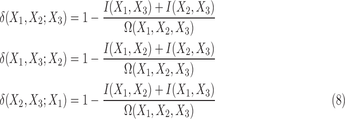Since both mutual information and multi-information are non-negative, and due to Equation (7), the range of the values of is seen to be . The value is 1 when the numerator goes to zero, while the denominator remains positive. Notice, however, the opposite is not possible: the numerator cannot remain positive when the denominator goes to zero. In the limit where the multi-information goes to zero, the mutual information also goes to zero, and the expressions in Equation (8) may not be well behaved. This will be considered later in data analysis applications. In the cases considered in this article, this presents no problem.

3. The Information Content in a Simple Function: Three Binary Variables (3 × 2)

The description of the information in a function can be complex, but while an overall single measure of collective dependency can be defined, dependencies among variables defined by the function cannot be fully characterized by a single quantity even for discrete functions. As noted in the previous section, for three variables, a full description involves at least three measures for the three-variable dependencies and three measures for the pairwise dependencies. Keep in mind, however, these are not independent measures, as is evident from Equation (8).

We consider first the simplest case of three binary variables, X, Y, and Z, where . This binary function can be represented by a logical truth table. Sixteen such functions, , are possible: all four possible values of mapping to two possible values of Z. To compute information measures on these functions, we convert each function f into a data set such that each triplet of values is copied an equal number of times, ensuring that X and Y are independent and equally distributed. We first consider the pairwise dependency measures.

3.1. The pairwise information landscape

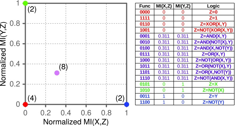
A typical approach to data analysis is to search for pairwise dependencies within the data. Note that this is a simplification. The genetic case, for example, cannot be fully described by a set of pairwise relationships. Consider the normalized mutual information (MI) between all possible pairs of variables within all possible 3 × 2 functions. Specifically, we compute MI scores for the possible pairs , , and for all 16 of these functions. Mutual information of is always zero since X and Y are independent by construction. Computing the mutual information of for all 16 possible functions reveals that 2 functions have full pairwise dependency between X and Z (); 8 functions have partial pairwise dependency (); and 6 functions have no dependency between X and Z (). Computing the mutual information of gives the same results due to symmetry. Plotting the and values of these 16 functions maps them to four distinct points; we can consider these points as defining four classes of functions, each class having the same mutual information values (Fig. 2). The and values in the plot are essentially the coordinates of the functions in the geometric landscape of pairwise relationships induced by these functions.

FIG. 2.

The landscape of pairwise information for all binary functions for three variables. There are 16 such functions and 4 function classes. The positions of the function classes are shown with colored circles, with the number of functions in each class indicated in parentheses. The table shows all 16 functions (using linear notation, Fig. 1) colored according to their assigned class, their coordinates, and the meaning represented using Boolean logic.

Each of the four classes of functions in the landscape is closed under permutation of values of X, Y, and Z. Moreover, the landscape is symmetric, and the diagonal is its axis of symmetry: any function of one class corresponds to a function of the reflected class by switching X and Y.

As expected, the asymmetric functions (those where one variable does not affect the functional relationship, such as when or ) lie at the corners of the landscape such that one coordinate is 1 and the other is 0 (colored green and blue in Fig. 2). An entire class of eight pairwise logical functions, such as , lie on the diagonal in the middle of the landscape (colored purple in Fig. 2). Note that exclusive OR (XOR)-type functions are located at the origin of the landscape (colored red in Fig. 2) together with all the constant functions (Z is the same for all X-Y combinations). This is not surprising since XOR is a special function that actually does not contain any pairwise information, only three-variable information, as the mutual information is zero for all pairs.

We can use mutual information to classify functions by their pairwise information based on their coordinates in the pairwise information landscape. On the other hand, mutual information is limited to identifying only pairwise dependencies. Higher order measures of variable dependencies (such as our delta scores) are needed to fully characterize the three-dimensional case.

3.2. The three-way information landscape

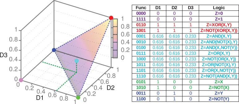
We continue our analysis by computing three-variable deltas, which measure nonpairwise dependence between variables. For each triplet of variables, , we compute three asymmetric delta measures [Eqn. (8) in Section 2.2] with each of the three variables being a target variable: , , and . As we will demonstrate, these three measures fully characterize the information content of the 16 functions. Note that this in turn would be a full description of the genetic example if the phenotype and genotypes were binary—described by only two possibilities. Similar to the pairwise case, we can construct a geometric information landscape of the functions by using these delta values as the coordinates (Fig. 3).

FIG. 3.

The three-dimensional cube of D₁, D₂, and D₃: the landscape of three-way information. The plane in which four of the five function classes (indicated by colored dots) lie is shaded. The gradient color, illustrating the slope of the plane, corresponds to the values of D₃. Similarly to that in Figure 2, the table shows details of all 16 functions colored according to their assigned class.

In the three-dependence case, the set of 16 functions falls into 5 distinct classes (each class has the same coordinates in the three-dimensional cube, Fig. 3). As in the pairwise case, all of the function classes are closed under permutation of variables X, Y, and Z. The class of functions located at the origin of the cube (a purple dot in Fig. 3) is trivial, consisting of only constant functions; that is, Z is a constant for all pairs of . The other four classes lie on the same diagonal plane shown in Figure 3. The fact that these functions all lie on the same plane can easily be seen using the definition of delta and independence of X and Y. Since X and Y are independent, and Equation 8 then define a plane since there are only two linear variables, and . Note also that there is symmetry in the plane since X and Y are interchangeable. The line passing through cyan and red dots is the axis of that symmetry: green and blue dots are reflections of one another. The functions from classes colored cyan and red are inherently XY symmetric, lying on the axis of symmetry.

Notice that XOR and its negative are located at the very top of the triangle (colored red in Fig. 3). On the other hand, completely pairwise functions, such as , are located at the bottom two corners (in blue and green), and the functions that contain the mixture of pairwise and nonpairwise information, such as , are located in the middle (in cyan, Fig. 3). Therefore, the values of D₁, D₂, and D₃ in Figure 3 are the coordinates of the functions in the landscape of three-way nonpairwise information induced by these functions. These coordinates reflect the amount of XOR-like information encoded in the functions.

Although this set of binary functions represents a very simple example, it is surprisingly rich in content. This example shows that deltas and mutual information can be used not only to detect functional dependence between variables but also to identify the class of functional relationship. This striking insight implies that we can identify a function class (or classes) from the mutual information (two-variable) and the delta (three-variable) coordinates derived from a data set. In principle, then, both the detection of dependence, using the symmetric delta (the product of D₁, D₂, and D₃, for three variables, Eqn. (3); Galas et al., 2014), and the nature of the dependence up to the class, using individual coordinates, can be obtained from already calculated information theory-based measures.

The examples so far have been very simple as the alphabet is limited to binary values. We now explore a more nuanced case using the more complex example of 3 × 3 functions, those functions of three variables with a three-letter alphabet.

4. Increasing Complexity: from Binary to Three-Valued Alphabets

The previous section showed that the information landscapes provide detailed information about the structure of binary three-variable functions and thus they are useful for uncovering the functional nature of dependencies. On the other hand, although binary phenotypes are important in genetics, the family of binary functions is limited. Increasing the alphabet size from two to three values yields more information-rich discrete functions, which are more relevant to biology. These discrete functions are similar to many genetic functions, where the genotypes at two loci are X and Y and the phenotype is Z, as we explore later.

Looking at the combinatorics of these families of functions, the number of three-variable functions is vastly larger with the increase of the alphabet. In general, the number of functions, N, with three variables X, Y, and Z such that , , and is . The 3 × 2 case of Section 3, consisting of three binary variables, yields only functions. However, when we increase the number of values of a variable from two to three values, the number of all possible functions increases dramatically. If we keep variable Z binary, but allow X and Y to be ternary, the number of functions increases to , and if we allow all variables to be ternary, then this number jumps to . In the case where the variables can take on four values, there are over 4 billion functions.

In this article, we will consider only the binary and ternary variables. First, we will take a quick look at the case when X and Y are ternary, but Z is still binary. Then, we will study in depth the case when all variables are ternary.

4.1. The information content of simple functions: ternary X, Y, and binary Z

Let us consider another special family of functions, two 3-valued variables X and Y (representing genotypes) and one binary variable Z (representing a phenotype). This is an intermediate between 3 × 2 (all binary) and 3 × 3 (all ternary) cases. We will refer to it as the 3-3-2 case. There are 512 such functions.

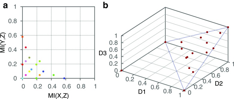
Computing mutual information coordinates for every 3-3-2 function yields a pairwise information landscape, shown in Figure 4(a). The pairwise information landscape consists of 16 classes: 6 classes on the diagonal and 5 classes on each side of the diagonal (they are reflections of one another due to XY symmetry).

FIG. 4.

The information landscape for the 3-3-2 case. (a) Five hundred twelve functions fall into 16 classes in the landscape of pairwise information. The positions of function classes are shown in (randomly assigned) colors. (b) The same family of functions is clustered into 17 classes lying in the cube of D₁, D₂, and D₃: the landscape of three-way information. The plane in which 16 of the 17 function classes (indicated by red dots) lie is outlined in blue.

Similarly, computing delta coordinates for every function in our family results in 17 function classes, one of which lies at the origin and the other 16 lie on a plane in a three-dimensional cube, forming the three-way information landscape (Fig. 4(b)). Details about the function classes and their correspondence between each landscape are provided in Appendix C.

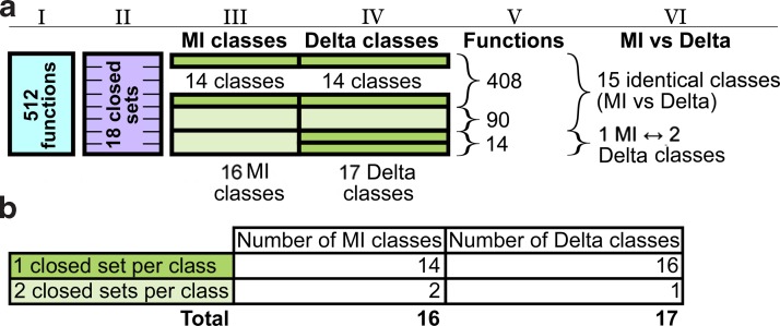
Note that each function class in both landscapes is closed under permutation of values of X, Y, and Z. There are 18 distinct permutation-closed sets, more than the number of classes in each landscape, which means that some classes comprise multiple permutation-closed sets. As illustrated in Figure 5, there are two classes in the pairwise landscape that consists of two permutation-closed sets each and one such class in the three-way landscape. What this means practically is that the mutual information coordinates alone allow us to correctly identify the closed sets for 14 function classes. Moreover, if we use delta coordinates, this number increases to 16, which illustrates that the three-way landscape is able to identify the nature of a dependency better than the pairwise landscape. Note, however, although there are classes whose closed set identity is ambiguous, identifying these classes still allows us to reduce the number of possible functions considerably. For example, the only class containing two permutation-closed sets in the three-way landscape reduces the number of possible functions from 512 to 90 (Fig. 5).

FIG. 5.

(a) Schematic illustration of the breakdown of the total set of 3-3-2 functions by closed sets (closed under variable permutation), MI classes, and Delta classes and the correspondence between the MI and Delta classes. The set of all (512) functions (represented by column I in blue) is partitioned into 18 sets closed under the permutation of variable values (represented by column II in purple). The closed sets are then grouped into either 16 MI classes or 17 Delta classes represented by columns III and IV correspondingly. The sizes of the multicolored segments in columns III and IV show how many closed sets the corresponding classes contain. The colors of the segments are defined in panel (b). The order of closed sets being grouped is the same between MI and Delta classes, so columns III and IV illustrate how the MI and Delta classes correspond to one another: 15 classes are identical between MI and Delta landscapes, and 1 MI class is split into 2 Delta classes (as pointed out in column VI). Column V also shows how many functions are contained in different groups of classes. (b) Color scheme of the classes by the number of closed sets contained in them and the corresponding number of MI and Delta classes.

The next section shows that all these considerations become much more complex when we simply increase the alphabet size of variable Z from 2 to 3.

4.2. The information content of simple functions: the 3 × 3 case

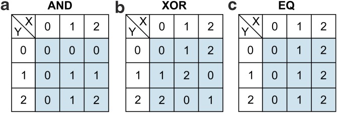
Let us now consider the case where all three variables, X, Y, and Z, are three valued and , with X and Y independent as in section 3. Each of these functional relationships can be represented by a 3-by-3 table, which can also be seen as an extended version of a truth table. This case corresponds to the genetic example in the introduction. For example, Figure 6 shows three functions that can be seen as extensions of the truth tables for logical AND, logical XOR, and equality (EQ) functions.

FIG. 6.

Examples of extended (3-by-3) truth tables defining three-valued versions of (a) logical AND, (b) XOR, and (c) EQ functions.

Note that these functions can be unambiguously represented in our linear notation as 000011012, 012120201, and 000111222, correspondingly (Fig. 1). We call the function defined in Figure 6(a) an extended AND because the lower value of the two arguments dominates, similarly to the binary version. The extended XOR function is more interesting. As in the binary case, each value of the ternary XOR is defined strictly by both argument values. In other words, information about one argument of the XOR function does not provide any information about the output value of the XOR function. This general scheme can also be considered as implementing a three-valued logic. It is similar to many genetic functions, where the genotypes at two loci are X and Y and the phenotype is Z. We will return to the genetic functions in a later section.

The set of all possible functions of this nature is much larger than the binary case of 16 functions or the 3-3-2 case of 512 functions. There are 19,683 possible functions in the 3 × 3 case, which is large, but is still relatively modest and small enough to be enumerated and classified.

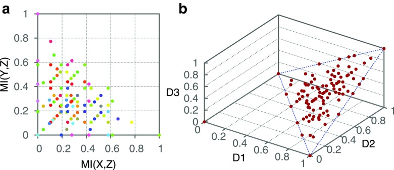
As in the 3 × 2 and 3-3-2 cases, we construct the pairwise and three-way information landscapes by computing normalized mutual information and delta measures and using them as coordinates. Figure 16 in Appendix D shows that these landscapes are very similar to those constructed in the previous two cases, but much denser in function classes due to higher complexity of the functions. The entire set of 19,683 functions falls into 100 pairwise and 105 three-way classes. Appendix D gives the full description of both these landscapes and their properties.

FIG. 16.

The information landscapes for the 3 × 3 function case. (a) 19,683 functions split into 100 classes in the landscape of pairwise information. The positions of the function classes are shown in circles with randomly assigned colors. (b) The same family of functions is clustered into 105 classes (indicated by red dots) lying in the cube of D₁, D₂, and D₃: the landscape of three-way information. All nontrivial functions lie on a plane outlined in blue.

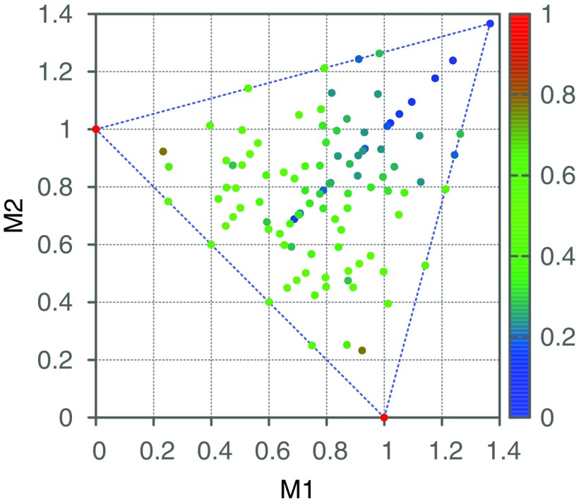
In general, while navigating the landscape of pairwise information, we find that the functions at the origin contain no pairwise information, and the further away from the origin we are, the more pairwise information we have between two variables. By rotating the diagonal plane of the three-way landscape onto the XY plane and coloring all the classes according to their pairwise information content (the maximal amount of MI provided by the functions), we can further see the distribution of the pairwise information in the landscape of three-way information (Fig. 7).

FIG. 7.

The landscape of three-way information after rotation. Rotation of the three-dimensional space defined by D₁, D₂, and D₃ so that all the points lie on the XY plane, using the transformation: and , where . The color bar map corresponds to for each function class, where the maximum is taken across all MI values of all the functions of a class.

Figure 7 shows the change in balance between pairwise and three-way information as we traverse the three-way landscape. The functions with the highest pairwise information (e.g., ) lie in the bottom corners of the landscape (). Moving away from the corners and toward the diagonal (including functions such as the extended AND) reduces the amount of pairwise information. Moving up to the top right corner (), functions approach the XOR-type function with zero pairwise information, but significant three-way information. This is an important class of functions in illustrating a common misconception. It is often assumed that pairwise information is sufficient to characterize most multivariable relationships. The XOR is the extreme example for which there is absolutely no pairwise information, but significant three-way information.

Similar to the previous cases, the set of all 3 × 3 functions can be grouped into a collection of sets, each of which is closed under permutation of values of X, Y, and Z. In this case, there are 139 such permutation-closed sets, and each of these sets can thus be represented by a single function in the group, from which all other functions of the set can be derived by variable permutation.

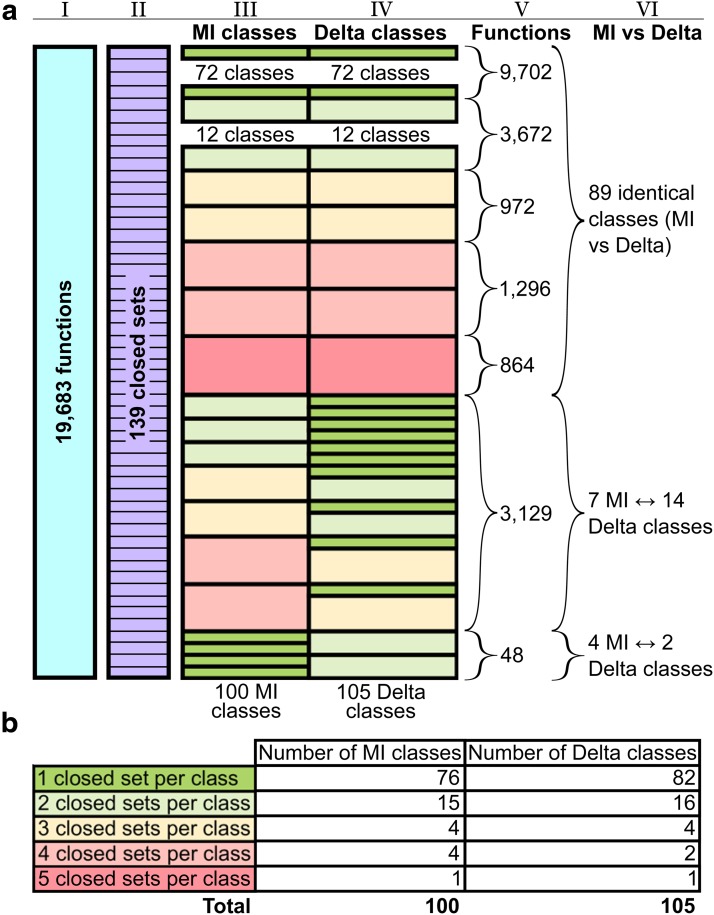
On the other hand, each function class identified from either the pairwise or three-way information landscape is closed under permutation of values of X, Y, and Z, which means that each class consists of all the functions from one or more permutation-closed sets. Since there are 139 distinct permutation-closed sets—more than the number of function classes in either of the landscapes, there are many function classes that contain multiple permutation-closed sets. Figure 17 in Appendix D illustrates the breakdown of all 3 × 3 functions by permutation-closed sets, pairwise classes, and three-way classes. This figure is similar to Figure 5, and comparing the two makes it easy to realize the amount of increased complexity going from the 3-3-2 case to the 3 × 3 case.

FIG. 17.

(a) Schematic illustration of the breakdown of the total set of 3 × 3 functions by closed sets (closed under variable permutation), MI classes, and Delta classes, and the correspondence between the MI and Delta classes. See Figure 5 for description. (b) Color scheme of the classes by the number of closed sets contained in them and the corresponding number of MI and Delta classes.

From Figure 17, we see that there are a number of classes in both landscapes that consist of multiple closed sets. Note, however, the majority of them consist of only two sets. This means that the coordinates of the functions in these classes considerably narrow the possibilities when determining the closed set identity of these functions.

Note also that the three-way information landscape distinguishes the closed set identity of the functions more completely and precisely than the MI plane coordinates. Figure 17 illustrates this clearly. In the pairwise information landscape, there are 89 classes (call these pairwise classes) that are identical to the classes in the three-way information landscape (call these three-way classes). However, there are seven pairwise classes that map into two different three-way classes. For the 3129 functions in these 7 classes, the delta coordinates thus do a better job of distinguishing the closed sets than the MI coordinates.

4.3. The delta as a function class lookup table

It is clear from the previous section that both mutual information and three-variable delta provide important information theoretic measures of dependency and can be used successfully to detect various classes of functional dependency. However, these measures target two distinct types of information, namely the information induced by pairwise dependence on the one hand and three-way information, which involves collective and nonpairwise information, on the other. The XOR-like functions are at one extreme, with no pairwise dependence. Although these two types of information are overlapping, used together, they allow us not only to detect dependencies in the data but also to identify the function classes of the dependencies. This presents us with an interesting and powerful opportunity. While the symmetric delta allows us to detect dependencies no matter what the functional form may be, the quantities that compose the symmetric delta (the D_i) can be used to provide additional information about functional classes.

Taken together, these components provide a general information theory-based, integrated data analysis method, combining dependency and functional form determination. The component steps are as follows:

• 1. Given three discrete variables X, Y, and Z with a specified range, construct a lookup table of all coordinates of the functions (mutual information and three-way delta coordinates).

• 2. Calculate the symmetric delta to detect and identify a set of candidate dependencies and quantitate their dependence measures, applying the shadow algorithm to avoid the combinatorial explosion if necessary (Sakhanenko and Galas, 2015). Retrieve the MI and Delta values for all subsets considered significant.

• 3. For each such dependent subset, then simply identify the function classes using the MI and Delta values that are the closest on the map to the known dependency—that is, we simply look it up. We consider the effect of noise on this process in the next section.

Note that because of the nature of the function classes we have discussed in sections 4.1 and 4.2, even if the data are precise and voluminous enough to define information measures with high accuracy, there are classes of functions that have many members that cannot, even in principle, be distinguished using these measures.

This outline provides the framework for a practical analysis approach, but there are, of course, important practical issues as well. These include the presence of statistical fluctuations due to sampling and noise in the data that add uncertainty to the process of function class identification. This needs much more study. Let us address the noise issue first.

5. Application of the Information Map

In sections 3 and 4, we showed that by using mutual information and delta measures, not only can we detect dependency but we also can identify the function class of the dependency. In this section, we consider how the presence of noise in real data can affect the information landscapes and interfere with classification.

5.1. Data noise

We add noise here to a dataset otherwise completely consistent with a specific function. Consider an arbitrary function chosen from each closed set of every function class in the pairwise landscape. Adding noise to a function class is the same as adding noise to these arbitrary functions. To add noise to a function f, we convert f into a data set containing M copies of every possible triplet of values of X, Y, and Z according to the definition of function f. In other words, is a table with rows of data points, triplets of XYZ values. To compute a dependency measure on a function f, we apply the dependency measure to the set . We then randomize values of Z in the set for R randomly selected data points. 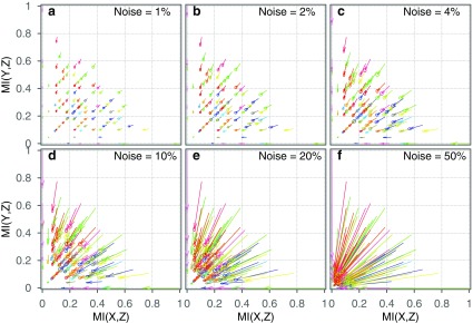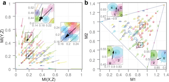This approximates the probability of a random Z. The mutual information coordinates of perturbed functions are then calculated. This randomization process is repeated K times, each time computing the mean and standard deviation of MI coordinates of an arbitrary function from a function class. Figure 8 shows the MI coordinates of each function class before and after the addition of noise visualized by the ends of arrows. The location of the arrowhead corresponds to the average MI coordinates of the class after different amounts of noise were added (six different noise levels) and the ellipse shows their standard deviation.

FIG. 8.

Effects of noise on each spot (function class) in the pairwise information landscape. For an arbitrary function f of each class, we create a data set and then randomize R randomly chosen Z values in the set. We repeat this process K times, each time computing the mutual information coordinates of the randomized function, and find the average and standard deviation of the mutual information coordinates. We show the results for (900 data points in each data set), , and [shown in panels (a–f) correspondingly]. Each arrow shows the shift of coordinates of a class after adding noise, and the ellipse at the end of each arrow represents the location of the average and the standard deviation of mutual information coordinates.

In Figure 8, it is clear that all the mutual information of classes moves toward a single point at the origin as the noise increases. The direction of the shifts induced by the noise is consistent across all classes. On the other hand, the magnitude of the shift differs markedly among function classes.

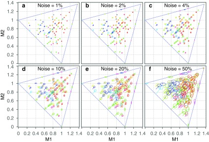
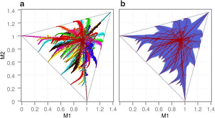
To track the noise effects on the three-way information landscape, we repeat the above noise-adding process for all function classes in the landscape. In Appendix E, Figure 21 shows the shifts resulting from six specific noise levels (parallel to Fig. 8), while Figure 9 shows the resulting trajectories in the 3 × 3 landscape as noise is added continuously. Note that the trajectories in Figure 9 are smooth curve fits to the averaged coordinates of functions in each class making it easier to see the trend of the movement. This plot shows how the position of the function class moves and how its location becomes increasingly uncertain as a function of the added noise level. Similar to the pairwise information landscape, all classes in the three-way information landscape move eventually to the same location, whose coordinates are around 0.92 (in the transformed plane). This position defines a complete loss of distinction among classes. On the other hand, the directions of the shifts of different classes are not at all linear as they are, approximately, in the pairwise case and define a rather complex trajectory for most classes. Moreover, the trajectories are more specific to each class than in the pairwise landscape. The way the variation ellipses change their size and shape is also different and specific to each class (Fig. 21). Notice also that the standard deviation increases more quickly with increasing noise than in the pairwise case, making it harder overall to distinguish the classes from each other. In general, it is more difficult to distinguish between function classes at moderate noise levels in the three-way information landscape than in the pairwise landscape.

FIG. 21.

Effects of noise on each class in the three-way information landscape. We systematically randomized the generator functions of each class similar to Figure 8 and computed the average and standard deviation of three-way delta coordinates. We show the results for (900 data points in each data set), , and [shown in panels (a–f) correspondingly]. Each arrow shows the shift of coordinates of a class after adding noise, and the ellipse at the end of each arrow represents the average and standard deviation of delta coordinates of a function with noise.

FIG. 9.

Trajectories of function classes in the three-way landscape with increasing noise. (a) All colored points correspond to delta coordinates of all function classes in the three-way landscape. Color is arbitrary and used simply to distinguish different function classes. We construct the trajectories of the function classes by increasing the noise level from 0% to 100% similar to the way it was done in Figure 20. Each smooth red line corresponds to a Bezier curve fit to all the coordinates of a function class. (b) Only Bezier curve fits for each function class (red) with half standard deviation of noisy coordinates are shown as transparent, overlapping purple ellipses.

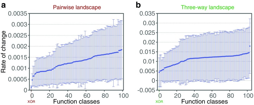
We calculate, in both landscapes, the rate at which a function class shifts in the landscape with the increase of noise. Figure 22 shows the average and standard deviation rate of shift for all classes in the ascending order for both landscapes. Four function classes with the least movement in the pairwise information landscape are {000000000, 012120201, 001010100}, {001001110, 001010101}, {001021110, 001011120, 001012110}, and {001012120, 001120210}. Note that the multiple functions in each class correspond to multiple closed sets that have the same coordinates in the landscape. In the three-way information landscape, the function classes with the least movement are {012120201, 001010100} and {000000111, 000111222}. Note that in both landscapes, the class with the smallest shift rate contains the three-valued XOR function (highlighted in bold).

FIG. 22.

The average and the standard deviation of the rate of shift of the function classes in (a) the pairwise and (b) three-way information landscapes. All the classes are ordered by the average rate.

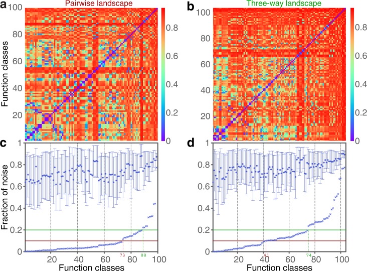
Given our analysis of the effect of noise on the functions in the information landscapes, we can now ask how easy it is to distinguish the function classes for different levels of noise. To answer this question, we determine the minimal level of noise at which two classes in the landscape overlap. We call two classes overlapping if the variation ellipse of one class overlaps with the ellipse of the other class at some noise level. The minimal noise level at which two classes overlap is the level of noise above which the corresponding function classes become indistinguishable. Figure 10(a, b) shows the heat maps of the minimal overlap noise levels for all possible pairs of classes in both landscapes. Figure 10(c, d) shows the mean, standard deviation, and minimum of the values in each column of the heat map.

FIG. 10.

Distinguishability of classes in the presence of noise. Panels (a) and (c) correspond to the pairwise information landscape, and panels (b) and (d) correspond to the three-way information landscape. Panels (a) and (b) are heat maps where the rows and columns correspond to classes in the landscape, and the color corresponds to the noise level at which two classes start overlapping. The rows and columns are ordered by the minimal noise level—the noise level at which a class starts overlapping with any other class. Panels (c) and (d) show the average, standard deviation, and minimum of the noise level for each class, ordered by the minimum noise level. The red and green lines correspond to the 10% and 20% noise levels, with the numbers indicating how many function classes have their minimum of the noise level below these levels (c: 73 and 88, and d: 41 and 74.)

The minimum noise level for a class in Figure 10 is the level of noise at which the corresponding function class becomes indistinguishable from another function class. The XOR function class has the largest minimum tolerable noise level of all function classes in both landscapes. This suggests that three-way dependence is statistically more robust to noise for classification than pairwise dependence, which may be useful in future work.

The bottom panels of Figure 10 show that the function classes in the three-way information landscape are more easily distinguished in the presence of noise than the function classes in the pairwise information landscape: there are 73 function classes in the pairwise landscape whose minimum of the noise level is below 10% compared with 41 such classes in the three-way landscape. For the noise level of 20%, these numbers are 88 and 74, respectively.

5.2. Mapping function classes with noise in the data

Given our analysis of the effects of noise on the function classes in the information landscapes and on our ability to distinguish one class from another, we can adjust the data analysis method from above to account for the uncertainty in the data. The noise-adjusted method includes the following:

• 1. Create a lookup table for each landscape such that for every location in the landscape (for every pair of coordinates), we know how likely it is that it belongs to a function class.

• (a) For every pair of coordinates in the pairwise landscape, determine the level of noise needed for a function class to overlap with this position. Repeat for every class in the pairwise landscape.

• (b) For every pair of coordinates in the three-way landscape, determine the level of noise needed for a function class to overlap with this position. Repeat for every class in the three-way landscape.

• 2. Apply the shadow algorithm (if needed) and the symmetric delta to detect a set of candidate dependencies (Sakhanenko and Galas, 2015), quantitate their dependence, and determine the significance.

• 3. For each such dependency, we find the sets of most likely function classes from the lookup table based on MI and Delta coordinates.

What will result from this procedure will be an increasing set of candidate classes as the noise increases, and the regions of ambiguity on the landscape map will be heterogeneous and rather complex. Let us now examine how these considerations apply to the real examples of genetic interactions.

6. Application to Genetics

From the discussions in sections 4.2 and 5, it is clear that even though the 3 × 3 case is simple and can be analyzed exhaustively, encompassing all possible functions, it is surprisingly complex and generates very diverse information landscapes. In this section, we show that the 3 × 3 case is also practically useful in biology, particularly in the field of genetics.

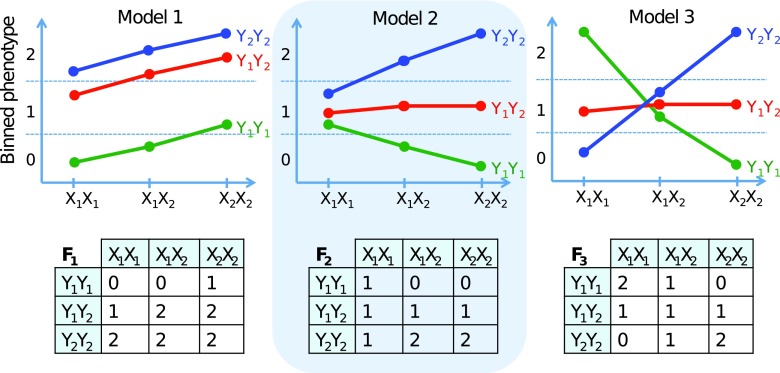
As illustrated by Mackay (2014), a pairwise gene interaction with a discrete phenotype can be represented as a three-valued function with two arguments. Figure 11 shows three examples of gene interaction with and without epistasis (Mackay, 2014) and their corresponding 3 × 3 function tables.

FIG. 11.

Three models of gene interaction effects of two genes on a three-valued phenotype (adapted from Mackay, 2014). The top three panels are graphical representations of the genotypic effects from variations at two loci, X and Y, using common genetic diagrams. The bottom three tables show the corresponding function that describes each case or each model. Model 1 shows additive gene effect at locus X, partial dominance at locus Y, and no epistasis between X and Y. Model 2 shows epistasis between X and Y such that the additive effect of Y alleles is greater in the genetic background than in the one. Model 3 shows epistasis between X and Y such that the additive effect of Y alleles in the background is opposite to the effect evident in the one.

To illustrate the application of our method in these cases, we generated a simulated dataset containing 20 three-valued variables, , and 180 samples. Variables are independent and uniformly distributed. Variables , , and take on the values of functions F₁, F₂, and F₃ correspondingly, as defined in Figure 11, with V₁ and V₂ being their arguments. Here, variables represent single-nucleotide polymorphisms (SNPs), and , , and represent phenotypes. The goal here is to detect the three SNP-SNP-phenotype dependencies and to identify their function classes.

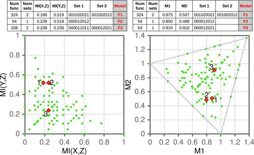
We start by computing mutual information and three-variable delta scores for all pairs and triplets containing one phenotype variable. Of 60 pairs and 570 triplets, there are 6 pairs and 3 triplets that are significantly different from the rest of the tuples (z-scores are over 10 for pairs and 100 for triplets). Using normalized mutual information scores as coordinates, the six detected candidate pairwise dependencies are mapped into the pairwise information landscape. Similarly, the three-candidate three-variable dependencies are mapped into the three-way information landscape using normalized three-variable delta scores as coordinates. Figure 12 shows that the three genetic models in our example fall into three distinct classes in the landscapes, allowing us to classify and partially uncover the identity of our functions (identifying only the class.) Tables in Figure 12 contain the information about each of the classes.

FIG. 12.

Information coordinates for the three models shown in Figure 11. Left: Normalized mutual information scores are mapped as coordinates for the six detected candidate pairwise dependencies in the pairwise information landscape (shown in red). Right: The three-candidate three-variable dependencies are mapped into the three-way information landscape using delta scores as coordinates.

Specifically, there are two pairwise dependencies related to Model 2, and , whose normalized mutual information is significant, 0.239 and 0.519 correspondingly (z-scores are over 10). Using these mutual information values as coordinates identifies the location of the dependency (Model 2) in the pairwise information landscape. Our model falls into class 2 containing a set of 54 functions closed under permutation of variable values. Note that although Model 2 can be any of the 54 functions from the class, all of the functions of the class are algebraically similar since the set is closed under permutation, so the identity of Model 2 is less ambiguous than it first seems.

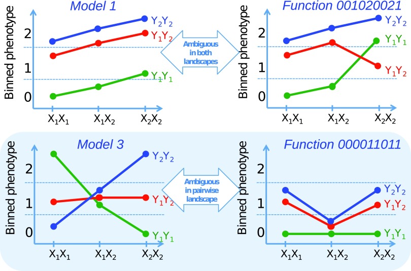
Similarly, the coordinates of Models 1 and 3 position them into classes 1 and 3 in the pairwise landscape correspondingly. Although this considerably reduces the uncertainty about which functions encode our models (324 and 108 possible functions of almost 20K), both classes contain two closed sets of functions each and it is ambiguous as to which of the two sets our models belong to. Figure 13 shows the nature of ambiguity of the functions.

FIG. 13.

An illustration of the ambiguity of function classes related to Models 1 and 3 from Figure 11. Model 1 is ambiguous in both pairwise and three-way information landscapes, while Model 3 is ambiguous only in the pairwise landscape.

The ambiguity of the function set membership of Model 3 is resolved when it is mapped to the three-way information landscape. The normalized delta coordinates of the Model 3 dependency position it inside of a class in the three-way landscape that contains only a single closed set—one of the sets from the class in the pairwise landscape Model 3 was mapped to. Not only does this reduce the number of possible functions to 54 but it also ensures that all these functions are algebraically similar. Mapping Model 1 and Model 2 dependencies into the three-way landscape results in the same set of functions as in the pairwise case. This also means that the ambiguity of the Model 1 functional identity remains—the corresponding dependency gets mapped to a class containing two closed sets of functions.

6.1. Effects of noise on inference of genetic function classes

The example above illustrates how by using our information theory method, we can successfully go from detecting a dependency to identifying a function class of the dependency. This example, however, is far from a real biological situation as it contains no uncertainty or noise. We now consider how added noise affects the performance of our method.

To add noise to a simulated example, we randomly select N samples of the total 180 samples and randomly permute the values of Z in the selected samples, where for a triplet under consideration. We repeat this random permutation 100 times for each class in a landscape (choosing an arbitrary function in the class), estimate the coordinates of the permuted function, and then compute an average and a standard deviation representing how much a class shifts position in the presence of noise. To illustrate a possible effect of noise on Models 1, 2, and 3, the function triplets corresponding to these models are randomly shuffled at some level. Figure 14 shows how adding 5.6% noise (shuffling 10 randomly selected samples) to the data affects the landscape and adds uncertainty to the process of identifying the function class of our three tuples.

FIG. 14.

The effect of noise on inferring genetic function class defined by the three models from Figure 11. The two panels show the pairwise (a) and the three-way (b) information landscapes. After adding 5.6% of noise, the lines and ellipses, representing the average shift and variation of each class in the landscapes, are computed similarly to those in Figures 8 and 21. The black arrows show the shift of the three models F₁, F₂, and F₃ defined in Figure 11 after adding noise. The insets show close-ups of the areas of interest. The concentric ellipses in the insets correspond to 0.5 and 1 standard deviation. The color is assigned randomly to better distinguish the classes from one another.

It is clear that adding noise increases ambiguity that makes it harder to correctly identify the function class of the dependency and that it depends on the map location. Table 1 summarizes the function classes identified for each of our genetic functions F₁, F₂, and F₃. Note that the true function class was among the identified classes for every function. On the other hand, the identity of every function detected from the landscapes contained ambiguities—there were classes that our functions were confused with (Table 1). Note, however, although there are ambiguities in the exact function identities, we are able to identify a very small subset of potential functions, which our functions could belong to given the noise threshold.

Table 1.

The Summary of the Classes from the Information Landscapes That are Within Two Standard Deviations from F₁, F₂, and F₃

Pairwise			Three-way
Confused with	Belongs to		Belongs to	Confused with
m34	m61	F1	d62	d6, d34, d96
m61	m34	F2	d34	d12, d56, d61, d96
m9, m10, m11, m17, m38, m59, m79	m23	F3	d35	d17, d60, d72, d89, d90

All the coordinates and standard deviations are computed after adding 5.6% of noise. The classes in the columns “Belongs to” are the true classes—the classes our functions belong to without noise. The classes in the columns “Confused with” are the classes our functions can be mistakenly assigned to due to added noise.

The location of function F₁ with noise in the pairwise landscape is less than one standard deviation away from its true function class. At the same time, F₁ is also located less than two standard deviations away from the function class that corresponds to function F₂. The accuracy required for unambiguous class identification clearly is location specific as shown by the examples for each of the model functions.

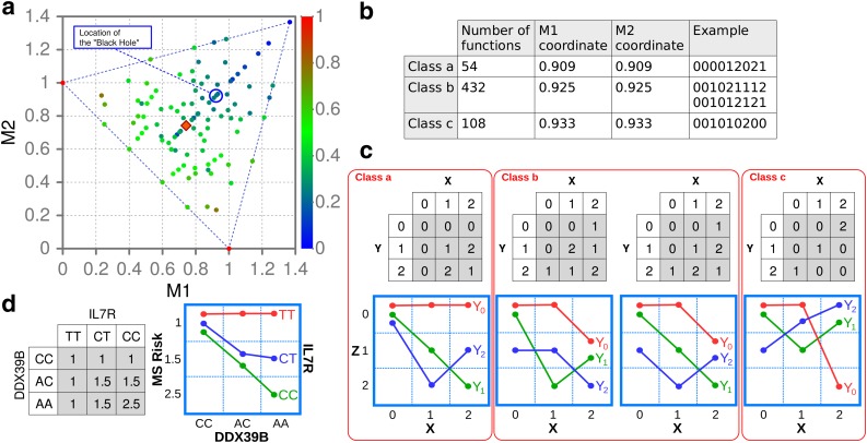
What is clear from the above considerations is that the information landscape for gene interaction functions is highly nonuniform, and the ambiguity ranges from very low to very high. As we saw in Figure 9 (showing the effect of increasing noise on the function classes in the three-way information landscape), there is a centrally positioned point in the landscape toward which all class trajectories converge as noise increases. Near this region, the ambiguity and noise sensitivity are very high. At the limit of complete loss of identifying information, the functions converge to a point on the plane that we call the black hole of information. As noise increases to high values, the position of any function moves near this point. In Figure 15(a), we indicate this point with the blue circle on the central axis. There are three classes of functions very close to this convergence point, which we identify in Figure 15(b).

FIG. 15.

There are three function classes very near the convergence point or black hole of information. (a) A blue circle shows the location of the convergence point relative to the function class locations. The orange rhombus indicates the location of the MS genetic interaction defined in panel (d). (b) The table shows the coordinates and the number of functions for the three classes from the blue circle. Classes a and c contain one closed set, whereas class b contains two closed sets. A function example is shown for each closed set. (c) The table representation of four example functions near the black hole (the blue circle) and their gene interaction diagrams. (d) Gene interaction in multiple sclerosis risk (its discretized form) between receptor gene, IL7R, and RNA helicase gene, DDX39B, reported by Galarza-Muñoz et al. (2017), shown as a table and as an interaction diagram. The location of the MS genetic interaction function is indicated by the orange rhombus on the information plane (a). This interaction mode is almost identical to the genetic interaction functions usually termed “Synthetic Lethality” and “Dominant Epistasis.”

These functions are the most difficult to distinguish from any other because of their proximity in the information plane and their sensitivity to noise. It is noteworthy, as shown by the gene interaction diagrams of these functions in Figure 15(c); these modes are similar to some of the most commonly cited examples of gene interaction.

As a further example, we examine a recently reported gene interaction that affects susceptibility to multiple sclerosis (Galarza-Muñoz et al., 2017). These interactions, inferred from the article and shown in discrete form in Figure 15(d), are very close in form to a few very commonly cited gene interaction modes; that is, the mode of synthetic lethality or more generally the synthetic interaction, in which the phenotype manifests only (or almost only) when a specific genotype occurs in both the genes. This is also called dominant epistasis. Both terms have been used to describe genetic effects in several domestic animals and plants, as well as in model organisms and in cancers. It is interesting that this relatively common interaction mode is located on the central axis of the landscape and that there are 216 functions in this class.

7. Discussion

There are three key problems at the heart of data analysis: detection of variable dependence, estimation of the significance of such dependence, and inference of the functional form of the dependence. In previous work, we have argued that an information theory approach allows separation of the detection problem from inference of the functional form problem. In this article, we begin to tackle the latter problem by presenting a direct method, based on information theory, for classifying the functional forms of intervariable relationships within a dataset. Our purpose is to lay the foundations for information-based methodologies rather than describing detailed analysis methods. We have limited our considerations to discrete functions, with up to three-variable dependencies, and with an alphabet of values of size two or three. We used a set of simple information measures to define information landscapes for such functions and showed that for an alphabet size of three, the 19,863 possible functions are naturally grouped by their information contents into only 105 classes in the three-way information landscape. These function classes lie within a two-dimensional subplane of this three-dimensional space, yet the complexity of the corresponding information landscape is surprising. When the effect of noise on the function classes of this landscape is examined, we see that the landscape is even more highly heterogeneous and exhibits strong nonlinear responses to noise.

Discrete variables are frequently encountered in data analysis, both due to the inherently categorical nature of the variables used and as the result of the binning of numerical variables into discrete integral alphabets. We have reviewed the information measures of dependence and proposed normalization schemes for the functions of up to three variables. The fundamental question of how much information resides in a given function is answered in the case of these discrete functions, and their surprisingly complex relationships have been shown to form sets of points on a planar information landscape that correspond to function classes. While the symmetry of the plane is evident, the total of 19,683 functions falls into 100 (pairwise) or 105 (three-way) function classes with identical information coordinates. The effect of noise on the inference of function class was also found to be highly heterogeneous. When we tracked the trajectories of the function classes as their coordinates shift under the imposition of increasing noise, some remarkable nonlinear trajectories that have heterogeneous properties (in the case of three-way information) were revealed.

We applied this approach to an important area of biological data analysis—that of genetic interaction analysis. Genetic analysis problems provide a rich source of real and complex biological data analysis challenges, and our general methods provide direct analytical tools for characterizing genetic problems and for analyzing genetic data. We illustrated the functional description and classes of a number of common genetic interaction modes. The degree of heterogeneity of the classes in their sensitivity to noise provides a caution in inferring genetic interaction modes and also suggests some interesting observations and principles. Well-known genetic interaction modes can be placed on the landscape and the noise sensitivity described. It appears that for functions with a strong imbalance of three-way dependence over pairwise dependence, the functions are more highly resistant to ambiguity induced by noise. The central point in the information plane to which all functions migrate as noise increases is an interesting phenomenon whose full meaning remains to be uncovered. We suggest that for higher dimensions (numbers of variables), there are similar points with similar singular behavior of functions.

Although our approach to analyzing the information content of functions is promising, many questions remain open. It is clear from Sections 5.1 and 6.1 that determining the class of a dependency in the presence of noise is a challenging problem and requires further detailed analysis. It is clear from the genetic example in Section 6.1 that a dependency function placed in a class using the information coordinates might, in fact, be from another class: the noise in the data could shift the dependency's coordinates sufficiently to result in the erroneous class assignment. Note, however, each class requires a different noise level for its coordinates to shift sufficiently to cause a misassignment. Therefore, given the information coordinates of a dependency, we can estimate the likelihood of the dependency assignment to a specific class. The analysis of the effects of noise on each function class and the estimation of such likelihood are topics for future research. A related question, and another future direction, is how to estimate a minimal amount of noise needed to shift a class to a given point. If, for example, we detected a dependency whose coordinates place it in an empty area of the information landscape (Fig. 9(b)), then we need to estimate how much noise we need at minimum for a function from any class to get shifted to these coordinates.

Note also that identifying a function class of a dependency is a significant step toward learning a model describing the dependency, which in turn can be seen as an encoding of the dependency data. Therefore, the exploration of connections between information landscapes of different function families and the capacity of these function families measured by the Vapnik-Chervonenkis dimension, defined for such considerations in learning theory, should provide us with links between information complexity and predictability of functions (Bialek et al., 2001) and thus is another important area for future research.

8. Appendix

8.1. Appendix A: The relationship between multi-information and interaction information

In the main text, we show the relationship for the three-variable case. For the four-variable case, the relationship is simple to calculate directly

which leads us to infer the general case for variables. Although we will not use it in this article, this is an interesting and rather simple relationship. The proof is direct from the definitions:

where the sum is over all subsets except the complete set, as indicated, and the one-element sets (single variables).

8.2. Appendix B: Proof of the non-negativity of

By definition,

From the definition of entropy, we have

Note that Equation (B2) becomes an equality if Y is independent of X. From Equations (B1) and (B2), it is clear that must be non-negative.

8.3. Appendix C: The details of the 3-3-2 case

The set of 3-3-2 functions consists of 512 functions whose variables X and Y (representing genotypes) are three valued and the third variable Z (representing genotypes) is binary.

The pairwise landscape in this case consists of 16 function classes (Fig. 4(a)). Because of XY independence, there are six classes that have full XY symmetry—they lie on the diagonal. The other 10 classes can be viewed as five pairs that are reflections of one another.

There are three classes of functions lying on the X-axis (), with different values of mutual information between X and Z, including the XOR function that has no pairwise information () and the function whose entire information content is pairwise (). Due to symmetry, the same relationships hold for the Y-axis. Table 2 contains detailed information about the function classes and their coordinates.

Table 2.

Information Landscapes in the 3-3-2 Case

Pairwise information landscape						Three-way information landscape
N. func	N. closed	MI (X, Z)	MI (Y, Z)	Examples		Examples		N. func	N. closed	Delta 1	Delta 2	Delta 3	M1	M2
18	1	0.1244	0.1244	000000001			000000001	18	1	0.6082	0.6082	0.2165	0.6875	0.6875
18	1	0.2890	0.0959	000000011			000000011	18	1	0.4005	0.8011	0.2016	0.4743	0.8749
6	1	0.5794	0.0000	000000111			000000111	6	1	0.0000	1.0000	0.0000	0.0000	1.0000
18	1	0.0959	0.2890	000001001			000001001	18	1	0.8011	0.4005	0.2016	0.8749	0.4743
36	1	0.0959	0.0959	000001010			000001010	36	1	0.8011	0.8011	0.6022	1.0215	1.0215
72	1	0.1931	0.1931	000001011			000001011	72	1	0.6667	0.6667	0.3333	0.7887	0.7887
36	1	0.1931	0.0000	000001110			000001110	36	1	0.6667	1.0000	0.6667	0.9107	1.2440
36	1	0.4322	0.0459	000001111			000001111	36	1	0.3089	0.9266	0.2354	0.3950	1.0127
18	1	0.2390	0.2390	000011011			000011011	18	1	0.6177	0.6177	0.2354	0.7039	0.7039
36	1	0.2390	0.0459	000011101			000011101	36	1	0.6177	0.9266	0.5443	0.8169	1.1258
6	1	0.0000	0.5794	001001001			001001001	6	1	1.0000	0.0000	0.0000	1.0000	0.0000
36	1	0.0000	0.1931	001001010			001001010	36	1	1.0000	0.6667	0.6667	1.2440	0.9107
36	1	0.0459	0.4322	001001011			001001011	36	1	0.9266	0.3089	0.2354	1.0127	0.3950
90	2	0.0459	0.0459	001010101	001001110	001001110	001010101	90	2	0.9266	0.9266	0.8531	1.2388	1.2388
36	1	0.0459	0.2390	001010011			001010011	36	1	0.9266	0.6177	0.5443	1.1258	0.8169
14	2	0.0000	0.0000	001010100	000000000		000000000	2	1	0.0000	0.0000	0.0000	1.0000	1.0000
							001010100	12	1	1.0000	1.0000	1.0000	1.3660	1.3660

Similarly, there are six classes lying on the diagonal (). If we start at the origin, where XOR and constant function lie, and move toward the center along the diagonal, we increase the pairwise information between X and Z and between Y and Z in a symmetric manner. The function on the diagonal most distant from the origin corresponds to a function with the largest amount of pairwise information when a function is symmetric. Note that due to independence of X and Y, only a limited amount of mutual information is possible between X and Z or Y and Z, so the most distant diagonal class cannot be at the maximum, .

In general, navigating the map of pairwise information, we find that the functions at the origin contain no pairwise information, and the further away from the origin we are, the more pairwise information we have between two variables. For more details about the classes, their functional content, and their coordinates, see Table 2.

Similarly, we can compute three-variable delta measures, the asymmetric measures D₁, D₂, and D₃, for each function, and construct a landscape of functions using these delta values as coordinates (Fig. 4(b)). The set of 512 functions is clustered into 17 distinct classes in the three-dimensional unit cube. All nonconstant functions lie on a diagonal plane, and the set of constant functions lies in the origin of the cube, away from the plane.

As in the previous cases, the three-way information landscape is XY symmetric, where the diagonal of the plane is the axis of symmetry. The 6 functions on the diagonal are all XY symmetric functions. Table 2 shows details of the function classes of the three-way landscape. The functions with the highest pairwise information (such as ) lie in the bottom corners of the landscape (when ). Moving away from the corners and toward the diagonal (toward functions that resemble logical AND function) reduces the amount of pairwise information. Moving up to the top corner () approaches the functions that resemble the logical XOR function that contains no pairwise information, but significant three-way information.

8.4. Appendix D: The details of the 3 × 3 case

8.4.1. Pairwise information landscape

The set of 3 × 3 functions consists of 19,683 functions, where all three variables, X, Y, and Z, are three valued and , with X and Y independent as in section 3. As a result, the pairwise landscape is fully characterized by and and is shown in Figure 16(a) (just like in the 3 × 2 and 3-3-2 cases). The entire set of 19,683 functions falls into 100 classes in this plane. That is, there are 100 sets of functions with identical mutual information coordinates.

Because of the XY independence, the pairwise landscape is symmetric as before (Fig. 16(a)). There are 18 function classes that have full XY symmetry and lie on the diagonal. The other 82 function classes can be split into 41 pairs that are reflections of one another (Supplementary Table S1 of function classes and their mutual information and delta coordinates).

There are seven classes of functions lying on the X-axis (), with different values of X-Z mutual information. The functions of this extreme range include both the XOR function that has no pairwise information () and EQ that has the largest amount of pairwise information (). Symmetry dictates the same relationship to the Y-axis.

Similarly, there are 18 classes lying on the diagonal (). As we move along the diagonal away from the origin, where XOR and a constant function lie, and move toward the center, we increase the pairwise information between X and Z and between Y and Z in a symmetric manner. The function at the most distant point on the diagonal () corresponds to a function with the largest amount of pairwise information when the function is symmetric. Since X and Y are independent, there is a limited amount of mutual information possible between X and Z or Y and Z, so the most distant point cannot be at the maximum, and . Another class on the diagonal contains the extended AND function among others.

As we said in the main body of the article, all 3 × 3 functions can be grouped into 139 sets, each of which is closed under permutation of values of X, Y, and Z. Each function class is closed under permutation of values of X, Y, and Z, which means that each class consists of all the functions from one or more permutation-closed sets. As illustrated in Figure 17, 76 of the 100 classes include only a single permutation-closed set. The other 24 classes consist of multiple (2–5) closed sets (there are 63 closed sets that get merged with other sets). What this means practically is that the mutual information coordinates alone allow us to correctly identify the closed sets for 76 function classes. For the other 24 function classes, consisting of more than one closed set, computing mutual information is not enough to identify precisely the closed set of a function. As shown in Figure 17, 15 of these classes consist of 2 closed sets each, 4 classes consist of 3 closed sets each, 4 of 4, and 1 of 5 distinct closed sets. To be able to discern more detail and to distinguish different closed sets in these MI classes, we need more information. We thus need the three-way deltas to identify the class.

8.4.2. Three-way information landscape

Similarly to the previous case, we can compute three-variable delta measures, consisting of three asymmetric measures D₁, D₂, and D₃ for each function, and construct a landscape of functions using these delta values as coordinates (Fig. 16(b)). The set of 19,683 functions is clustered into 105 distinct classes in the three-dimensional unit cube. As before, all nonconstant functions lie on a diagonal plane, and the set of three constant functions lies in the origin of the cube, away from the plane. As in previous cases, the three-way landscape is XY symmetric, with the plane's diagonal being its axis of symmetry. The functions on the diagonal are all XY symmetric functions.

As in all previous cases, the distinct function classes in the three-way landscape are closed under permutation of X, Y, and Z. The majority of the classes (82) consist only of the functions from one closed set, and the delta coordinates of the functions from these classes (a total of 11,053 functions) uniquely indicate their closed set identity (Fig. 17). Although the other 23 classes consist of multiple closed sets, the majority of them (16) consist of only two sets. The remaining classes consist of only 3 (4 classes), 4 (2 classes), and 5 (1 class) closed sets. This means that the delta coordinates of the functions in these classes considerably narrow the possibilities when determining the closed set identity of these functions.

8.5. Appendix E: The effects of noise on the function classes

The random triplets result in samples of the triplet (since there are 9 combinations of the X and Y values). Since each combination of values X and Y appears in the sampling an equal number of times (M), the independence between X and Y is preserved. The values of variable Z in the sampling are randomly sampled from a uniform distribution. For each such random triplet, we compute mutual information coordinates and show it on the pairwise information landscape. Figure 18 shows the distribution of random function in the pairwise landscape for and 900.

FIG. 18.

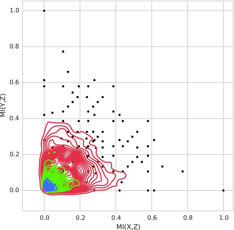
Pairwise information landscape with the background noise. We added 1000 random triplets and plot kernel density estimates (colored contours) in the pairwise landscape. To generate a random triplet, we first take all possible combinations of X and Y values (there are nine combinations), duplicate each combination M times (to preserve XY independence), and then draw random values of Z, one for each pair of XY values. For each random triplet, we computed its mutual information coordinates. We show the distribution of random triplets in the landscape for the sample size N equal to 18 (red), 36 (green), 90 (blue), and 900 (pink). Black dots correspond to the pairwise function classes.

Notice that in the pairwise landscape, the effect of the background noise is stronger when N is smaller, for example, 36 (of 100) classes are obscured by the noise when . In other words, when we do not have enough data, we can only detect dependencies with very large mutual information, and all other dependencies remain invisible. On the other hand, the effect of the noise decreases when N increases; for example, the number of obscured spots is 12, 2, and 1 for and 900 correspondingly.

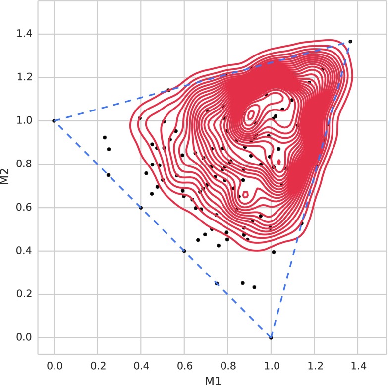
The distribution of random triplets in the three-way information landscape is rather different than that in the pairwise landscape. We computed normalized three-variable delta coordinates for the same set of random triplets for various N values as for the pairwise plot. In Figure 19, we show the distribution of the random triplets in the three-way information landscape for .

FIG. 19.

Three-way information landscape with background noise. Similar to Figure 18, we added 1000 random triplets and plot kernel density estimates (red contours) in the three-way information landscape. We generated a random triplet by constructing three random vectors corresponding to variables, X, Y, and Z, of the size N and computed their delta coordinates. The red contours show the distribution of random triplets in the landscape for the sample size N equal to 900. Black dots correspond to the three-way function classes.

Even for a very large N, the background noise does not localize to a small area in the landscape, unlike the behavior of noise in the pairwise landscape. The random triplets have very large fluctuations in the delta coordinates because of delta normalization. Equation (8) shows that normalization does not behave well when multi-information and mutual information get really small. Simple simulated examples reveal that the non-normalized delta is able to assign significantly high scores only to the dependencies in the data, whereas normalized delta correctly assigns high values (close to 1) not only to all these dependencies but also to many random tuples. The delta values of the random tuples, which are close to zero before normalization, range between 0 and 0.9 after normalization. It is clear that a non-normalized version of delta (symmetric delta) must be used when attempting to detect a dependency, but it then must be normalized to identify the function class of the dependency.

For each specific function, if we add noise and track the trajectory of the class, we see the changes as the mutual information coordinates decrease (Fig. 20).

FIG. 20.

Trajectories of function classes in the pairwise landscape as they track the increasing noise. (a) All colored points correspond to the MI coordinates of all function classes in the pairwise landscape. Color is arbitrary and used to better distinguish different function classes. We start with no noise and then gradually increase the level of noise to 100%, each time placing new points representing the shift of the coordinates of the classes due to noise. We kept the color consistent, allowing us to see a trajectory of each class under increasing noise. Each smooth red line corresponds to a Bezier curve fit to all the coordinates of a function class. (b) Only Bezier curve fits for each function class (red) with half standard deviation of noisy coordinates are shown as transparent purple ellipses.

Further exploration of the effect of noise involves the movement of function classes in the three-way information landscape as noise is added to the functions (Fig. 21).

The rates of change of the information coordinates of function classes as noise is added are important characteristics of the information landscape. As pointed out in the main text, the landscape is heterogeneous in this respect as well. One way of characterizing this property is to average the rate of change along the trajectories of each function class and to plot this profile as well as the variation in this average over the trajectory in terms of the standard deviation. These plots are shown in Figure 22 for the pairwise and three-way landscapes.

In the pairwise information landscape, 26 classes have the minimum of the noise level above 10% and 11 classes above 20%, whereas in the three-way landscape, 65 classes have above 10% and 29 classes above 20%. Note also that the average level of noise ranges between 60% and 80% in both landscapes, although both have complex structure (Fig. 22, and Fig. 10 in main text).

Acknowledgments

The authors acknowledge useful discussions about genetic applications with Joe Nadeau, Aimee Dudley, Jesse Riordan, and Gareth Cromie. This work was supported by the Bill and Melinda Gates Foundation, the NIH under 1U54DA036134 (DMRR), and the Pacific Northwest Research Institute.

Author Disclosure Statement

No competing financial interests exist.

References

- Bialek W., Nemenman I., and Tishby N. 2001. Predictability, complexity, and learning. Neural Comput. 13, 2409–2463 [DOI] [PubMed] [Google Scholar]
- Gacs P., Tromp J.T., and Vitanyi P.M.B. 2001. Algorithmic statistics. IEEE Trans. Inf. Theory. 47, 2443–2463 [Google Scholar]
- Galarza-Muñoz G., Briggs F.B., Evsyukova I., et al. . 2017. Human epistatic interaction controls IL7R splicing and increases multiple sclerosis risk. Cell. 169, 72–84 [DOI] [PMC free article] [PubMed] [Google Scholar]
- Galas D.J., Dewey G., Kunert-Graf J., et al. . 2017. Expansion of the Kullback-Leibler divergence, and a new class of information metrics. Axioms. 6, 8 [Google Scholar]
- Galas D.J., Nykter M., Carter G.W., et al. . 2010. Biological information as set based complexity. IEEE Trans. Inf. Theory. 56, 667–677 [DOI] [PMC free article] [PubMed] [Google Scholar]
- Galas D.J., Sakhanenko N.A., Skupin A., et al. . 2014. Describing the complexity of systems: Multivariable “set complexity” and the information basis of systems biology. J. Comput. Biol. 21, 118–140 [DOI] [PMC free article] [PubMed] [Google Scholar]
- Ignac T., Sakhanenko N.A., Skupin A., et al. . 2012. Relations between the set-complexity and the structure of graphs and their sub-graphs. EURASIP J. Bioinform. Syst. Biol. 2012, 13. [DOI] [PMC free article] [PubMed] [Google Scholar]
- Ignac T., Skupin A., Sakhanenko N.A., et al. . 2014. Discovering pair-wise genetic interactions: An information theory-based approach. PLoS One. 9, e92310. [DOI] [PMC free article] [PubMed] [Google Scholar]
- Li M., Chin L., Bin M., et al. . 2004. The similarity metric. IEEE Trans. Inf. Theory. 50, 3250–3264 [Google Scholar]
- Mackay T.F.C. 2014. Epistasis and quantitative traits: Using model organisms to study gene–gene interactions. Nat. Rev. Genet. 15, 22–33 [DOI] [PMC free article] [PubMed] [Google Scholar]
- McGill W.J. 1954. Multivariate information transmission. Psychometrika. 19, 97–116 [Google Scholar]
- Sakhanenko N.A., and Galas D.J. 2015. Biological data analysis as an information theory problem: Multivariable dependence measures and the shadows algorithm. J. Comput. Biol. 22, 1005–1024 [DOI] [PMC free article] [PubMed] [Google Scholar]
- Studený M., and Vejnarová J. 1999. The multiinformation function as a tool for measuring stochastic dependence, 261–297. In Jordan M.I., ed. Learning in Graphical Models. MIT Press, Cambridge, MA [Google Scholar]
- Watanabe S. 1960. Information theoretical analysis of multivariate correlation. IBM J. Res. Dev. 4, 66–82 [Google Scholar]
Associated Data
This section collects any data citations, data availability statements, or supplementary materials included in this article.