INTRAVITAL MULTIPHOTON MICROSCOPY AS A TOOL FOR STUDYING RENAL PHYSIOLOGY AND PATHOPHYSIOLOGY

Abstract

The kidney is a complex and dynamic organ with over 40 cell types, and tremendous structural and functional diversity. Intravital multi-photon microscopy, development of fluorescent probes and innovative software, have rapidly advanced the study of intracellular and intercellular processes within the kidney. Researchers can quantify the distribution, behavior, and dynamic interactions of up to four labeled chemical probes and proteins simultaneously and repeatedly in four dimensions (time), with subcellular resolution in near real time. Thus, multi-photon microscopy has greatly extended our ability to investigate cell biology intravitally, at cellular and subcellular resolutions. Therefore, the purpose of the chapter is to demonstrate how the use in intravital multi-photon microscopy has advanced the understanding of both the physiology and pathophysiology of the kidney.

INTRODUCTION

Microscopy as a technique has evolved past established tasks such as histological analysis of pathology specimens to one capable of simultaneously studying various dynamic cellular and subcellular processes in vivo. This is due to continuing improvements in optics, lasers, computers, and hardware. In turn, this has led to increased usage by making these complex systems far more affordable and robust while simplifying their ease of use. Studies utilizing intravital multi-photon microscopy (MPM) have increased because it affords the researcher data that is by nature dynamic, emanating from attached, intact, whole organs still regulated by intrinsic factors such as hormones, chemokines, and metabolites. The capability of imaging includes up to 4 channels simultaneously (blue, green, red, and far-red emitting fluorophores and compounds) at depth (3D) at near real-time speeds (4D data) thanks to innovations such as extremely fast resonant scanners on newer microscope systems and computers capable of rapidly collecting and storing these data sets that easily exceed several gigabytes in size. For example a 12-bit system acquiring three channels generates an ~1.5MB file per focal plane. Taking three 30μm volumes for 8 glomeruli at both 60× and 20× magnification plus an initial 200-frame infusion movie will exceed 1GB.

Our group has applied these techniques to studying renal physiology and pathophysiology within the intact, functioning kidney [1]. One limitation that varied from other organs previously studied, specifically the brain, is reduced optical penetration due to the increased cellular heterogeneity and blood flow of the kidney. Despite this limitation numerous studies have greatly advanced the understating of renal physiology and disease. Our study on fluorescent folate was the first to follow the transcytotic pathway of this essential vitamin after internalization by the proximal tubule. Previous studies relied on following the folate receptor due to the inability to fix folate in place for subsequent visualization via immunolocalization techniques [2]. Some of these discoveries have challenged long established dogma as disruptive technologies often do [3–8].

This chapter will review a number of techniques that focus on different aspects of renal morphology and physiology, and detail the methods used. The methods used to prepare the rat for imaging will not be discussed here having been carefully described in other publications [1, 5, 9]. First, an overview of the kidney structure, visualized by MPM, helps identify visual landmarks and establish differences between tubule types. Then studies that utilized numerous fluorescent probes to delineate various aspects of tubular function in health and disease will be reviewed. In particular, we will narrow our focus to the proximal tubule as the majority of studies have been on this segment of the nephron. This is the first part of the nephron to encounter the glomerular filtrate, and its functions to limit a wide range of important molecules and nutrients from being lost in the urine. Multi-photon microscopy quantitation of glomerular permeability, a key function of the kidney, will be described as well and key factors in assuring accurate measurement of this parameter.

Acute kidney injury (AKI) from renal ischemia and reperfusion (I/R) is an important area of study due to its clinical significance. Intravital MPM has helped elucidate a number of important findings relating to apoptotis and necrosis associated with ischemia/reperfusion. Alterations induced by this injury model that occur within the peritubular microvascular relating to red blood cell (RBC) flow, WBC rolling and adhesion, and vascular permeability can be studied using large molecular weight markers such as dextrans or albumin. One key finding made while utilizing this technique is the temporal and spatial heterogeneity in which intravenously infused fluorescent markers distribute throughout the microvasculature in pathologic conditions [10, 11].

These examples serve to underscore the novel, complementary approaches intravital MPM uncaps to advance an investigator’s research. However, they represent just a few examples of the true capabilities of this technique.

1). Morphology of the unlabeled renal cortex

Most modern turnkey confocal and multi-photon microscopes are equipped with an epi-fluorescent mercury arc lamp that allows for wide-field visualization and orientation of fluorescent samples prior to image acquisition. The standard filters typically included are a blue pass (for Hoechst and DAPI), a green pass (Fluorescein) and a red pass (Rhodamine and Texas Red), which will allow only those specific corresponding wavelengths through to the eyepiece. For intravital MPM it is highly advantageous to replace a filter (if necessary) with a dual pass red/green. The predominant feature of the kidney surface is the lysosomal autofluoresence localized within the proximal tubules facilitating their identification (Figure 1A and 1B). Autofluorescence has a broad red/green emission which gives it a combined yellow-orange color when viewed through a dual pass filter. The dual pass filter is useful when discriminating a true fluorescent signal (a dye or a fluorescent protein) from the red or green portion of the endogenous autofluorescence present in that particular band pass. Our laboratory sets red and green detector gain settings when acquiring images via confocal or multi-photon excitation to match the yellow-orange autofluorescent signal seen through the eyepiece. This normalizes the appearance of the images from experiment to experiment. Excitation power of the laser should be kept relatively low to prevent photo-toxicity. We typically keep laser power between 12-15% when using an excitation emission of 800nm. Power can be increased as longer, red-shifted excitation wavelengths are used because of a decrease in power output.

Figure 1.

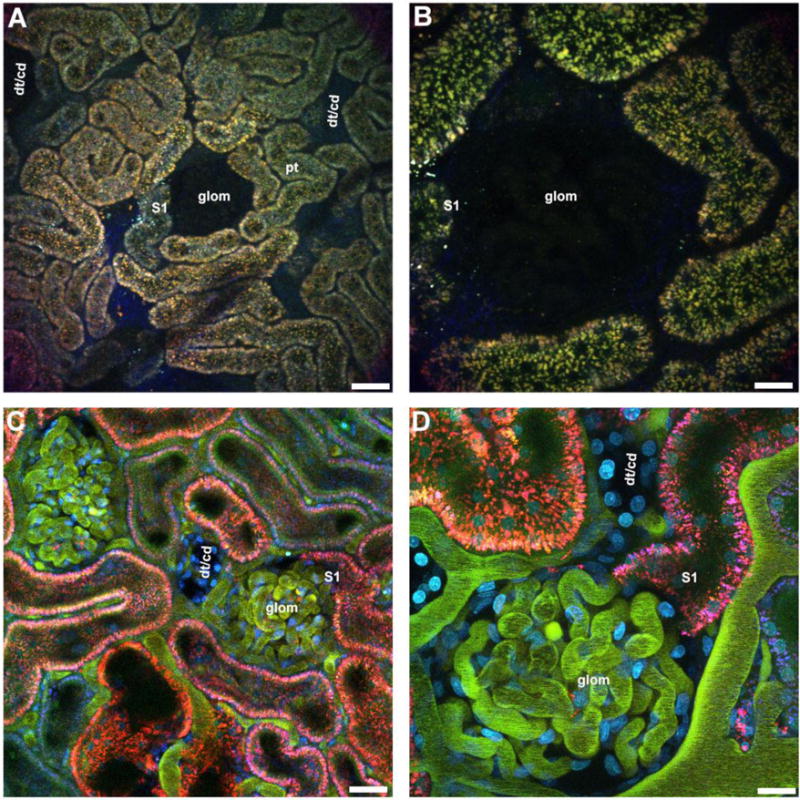
Outer cortical views. Proximal tubule autofluorescence on the rat kidney surface helps distinguish tubule types and other landmarks. Rats and mice have autofluoresence emanating from the lysosomes of proximal tubules (pt, orange vesicles). Distal tubules (dt) and collecting ducts (cd) lack any discernible autofluorescence and therefore appear as empty patches surrounded by the proximal tubule autofluorescence. Munich Wistar rats (panel A & B), as opposed to the other strains, have superficial glomeruli (glom) that also lack any discernible autofluorescence. The empty areas associated with glomeruli are typically circular and can be distinguished from the distal tubules/collecting ducts (dt/cd). About a third of glomeruli imaged will have the S1 segment of the proximal tubule visible. Panels C & D show a Munich Wistar rat that has been pre-injected with a 10kDa Cascade Blue dextran to label the PT lysosomes (blue), Hoechast 33342 to label nuclei (cyan), and a two rat serum albumins conjugated to either Fluorescein or Texas Red (appearing green in the vasculature). Note the appearance of the peritubular vessels and capillary loops that are now visible (green) as well as the cyan nuclei. Proximal tubules internalize the two differently labeled albumins, however due to the quenching of fluorescein emissions at the low pH of the endocytic compartment, only the Texas Red conjugate appears internalized (red). Panel A and C bar= 60μm, panel B and E bar= 20μm.

Other tubule types such as collecting ducts and distal tubules are indistinguishable from each other, lack any visible landmark and appear as large empty patches similar in size to proximal tubules. The Munich Wistar rat strains (Simonsen’s and Frömter) have in addition visualizeable surface glomeruli; the Frömter strain having roughly two to three times more than the Simonsen’s strain. Surface glomeruli lack any fluorescence and are discerned by the large circular void among proximal tubules (Fig 1A & 1B). Focusing through proximal tubules reveals the tubular lumen. A rough approximation of hydration status can be gauged by noting the lumen diameter. The lumenal space from a hypovolemic hypoperfused rat will be collapsed and the autofluorescent lysosomes will appear to touch from side to side. Surrounding the tubules is a network of peritubular capillaries and associated interstitial space. The use of a large molecular weight fluorescent dextran or protein will demarcate the vessel from the interstitial space (Figure 1C & 1D).

2.) Selecting a range of intensities for quantitation via Thresholding

Data obtained from intravital MPM is information intensive and quantifying a specific parameter can present challenges. Selecting regions of interest to quantify fluorescence intensity or area can be extremely labor intensive and time consuming especially if the areas are discontinuous. For example, drawing individual regions around endosomes in a field containing 60 cells, with 100 endosomes per cell, and analyzing 10 fields per condition (control and experimental) would make analysis prohibitively time consuming. Fortunately, many modern image processing and analysis software packages allow for quantitation of a selected range of intensities within an image while excluding the rest. This process would allow the aforementioned example to be analyzed in a few minutes by selecting the upper and lower range encompassing the endosomal associated fluorescence. After selection, parameters such as average fluorescence intensity, total thresholded area, total number of fluorescent spots, and average spot area (in pixels) are easily attained. In this chapter we will illustrate two examples of this technique. The first will be in the section detailing the method for quantifying the uptake of compounds within the proximal tubule via endocytosis. The second involves the determination of albumin plasma intensity within the renal vasculature where circulating RBCs blur the margins of the plasma. When conducting this analysis the user must be aware of the mode the software is in when reporting values. See figure 2.

Figure 2.

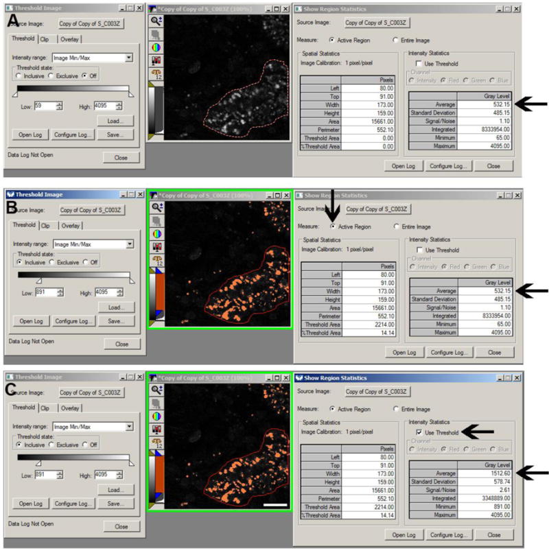
Fluorescence intensity thresholding. Thresholding allows for the selection of intensities for quantitation without having to outline multiple regions. Thresholding can be used to quantify the intensity for structures such as lysosomes by drawing a region around a cell or proximal tubule (panels A, B, and C, red outline). In panel A, no thresholding has been applied and the average intensity for the lysosomes shows a value of 532.15 fluorescence units (arrow). In panel B, a threshold mask has been applied to the image to include values between 891 and 4095 (left side of panel B). Although the threshold function has been applied the average intensity for the lysosomes still shows a value of 532.12 fluorescence units (lower arrow) because the dialog box on the right is still measuring the values for the entire selected region. Note the upper arrow in panel B showing the values are calculated for the selected region; if the “Entire Image” box is checked instead the values would represent the average of the whole image. In panel C, the “use Threshold” box has been checked (upper arrow) and the average intensity value for the lysosome is now 1,512.60 (lower arrow) since only the highlighted pixels are used in quantifying the value. (Bar= 20μm).

2.1

Drawing a region of interest around an area can be done in a stringent manner to trace a well-defined margin and isolate the area based on those margins. This is typically done when the entire region needs to be analyzed for area and/or intensity and there are structures in close proximity that have similar intensities. When drawing a region make sure the software is presenting values associated with that particular region only and not for the entire image.

2.2

When employing thresholding to select a range of intensities within a region, the margins of the region do not have to be drawn precisely if the intensity values between the area of interest and surrounding area vary markedly. When analyzing data in this manner, make sure the software is presenting values for that specific region and only for the intensities within the threshold. It is easy to overlook these subtle details and make errors in data collection.

3). Proximal tubule endocytosis and transcytosis

Materials

Small molecular weight dextrans 3kDa (Invitrogen, Carlsbad, CA) 4kDa (TdB Consultancy Uppsala, Sweden) 2.5-4.0 mg, Fluorescent albumin 2.5-4.0 mg.

One of the main functions of proximal tubules is the retrieval of fluid, electrolytes and macromolecules, that are filtered by the glomerulus, to prevent loss via urinary excretion. Once internalized across the apical membrane via receptor mediated or fluid phase endocytosis, endocytic trafficking within proximal tubule cells sorts material into two main pathways. These include sorting to the lysosomes for degradation and sorting to various other non-degradative compartments or locales within or across the cell. The inability of the proximal tubule to reclaim some of the filtered nutrients has been implicated in certain disease states and injury models. Intravital MPM has helped expand the investigative focus, beyond glomerular dysfunction, to elucidate the role tubular injury plays in proteinuric and albuminuric diseases that were previously thought to be associated solely with damage to the filtration barrier. In this section we will outline methods to study both pathways [8, 9]. In quantifying uptake, it is important not to saturate the intensity of the endosomal pool (particularly lysosomes) as this will underestimate the accumulation of the material therein [12]. Careful consideration to the background fluorescence must also be made when quantifying uptake of any compound into the lysosomal/endosomal pool. This value must be subtracted from the raw images to determine true and meaningful intensity values. See figure 3.

Figure 3.

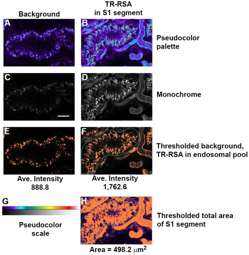
Quantifying cellular uptake of fluorescent compounds. Internalization of fluorescent compounds into proximal tubules can be quantified over time as progressive accumulation as a metric of injury or disease. Panels A and C show background images unrelated to panels B and D where Texas Red albumin has accumulated within the proximal tubule (center). Thresholding the background image in C shows an average background intensity of 888.8 fluorescence units which must be subtracted out from the thresholded image showing accumulation (panel F) with an average intensity of 1,762.6 fluorescence units. This background subtracted average intensity (873.8) is multiplied by the total number of pixels in panel F (801 pixels) to give total integrated fluorescence (TIF); 699,913. To normalize this value per unit area in a proximal tubule, the total area of the proximal tubule thresholded region in H (2913 pixels) is multiplied by the area of each pixel (0.171 μm²) to give a total area of 498 μm². Dividing TIF 699,913/498 μm² gives an area normalized value of 1,405 TIF/μm². (Bar= 20μm).

3.1

It is important to take several background 3D volumes of proximal tubules at three different laser illumination powers prior to initiation of the study to determine background values. These will be subtracted from the images showing accumulation of fluorescent compound taken at the matching laser power. In our studies we typically take 3D volumes at 15%, 12% and 9% laser power of the same background images and calculate average intensity values for each laser power. Doing so easily generates intensity correction factors between the different laser powers that can then be used to normalize background subtracted images taken at different laser powers. Determine background values for the corresponding laser power by thresholding to encompass the autofluroescence within the lysosomes for the respective channel (blue, green, red or far-red) depending on the fluorophore and noting the average intensity.

3.2

After designing a protocol to examine uptake, either various regions at a single time point or over time to show temporal accumulation, acquire images while being careful to minimize a large degree of saturation within the proximal tubule cells. As with the background images, threshold the image to encompass accumulated intensity within the endosomes, lysosomes and note the average value.

3.3

Subtract the average background intensity from the accumulated intensity of your compound to determine the corrected background-subtracted intensity. When following a temporal accumulation of a compound it may be necessary to lower the laser power used during image acquisition. If this occurs it is important to compensate for any decrease in laser power used over time in preventing signal saturation. Scale up any values that were collected at a lower intensity. To do so, compare the average intensity of identical non-saturated structures acquired at the different laser intensities. Calculate a correction factor by dividing the average intensity of the higher laser power image by the average intensity of the lower laser power image. This factor should be multiplied to the lower laser intensity image to scale the intensity values.

3.4

Average intensity values is one way of quickly presenting accumulation data. A more labor intensive method is to present the total integrated fluorescence (TIF). This value represents the average intensity multiplied by the area of fluorescence and is a better way of expressing this data because it will account for instances where a condition may induce an increase in the area of accumulation in addition to a change in the average intensity. The corrected value is attained by subtracting the background average intensity from the average fluorescence intensity of the accumulated compound. This figure is then multiplied by the total number of pixels used in generating the average intensity value. A note of caution; many software packages do present TIF as a value along with the area and average intensity; this value would be incorrect because it still contains the background intensity values. Total integrated fluorescence should then be normalized to the total area over which the value was measured. To do this, increase the threshold intensity to incorporate the area occupied by the proximal tubules in the quantified area. Note the area (presented in pixels), and multiply by the area in an individual pixel. For example an image taken using a 60× water immersion objective in our system will have pixel dimensions of 0.414 × 0.414 microns; an area equal to 0.171μm². Multiplying the total number of pixels by this factor will give you total area; 5,215 pixels × 0.171μm² = 891.7μm². Dividing the TIF by the area will give you a value that will normalize TIF differences in different areas between analyzed fields and best quantifies accumulation.

3.5

Transcytosis is not an event that is associated with many common markers that traffic through the endosomal pool and accumulate in the lysosomes [3, 7]. In our study of albumin trafficking we noted finger like projections and vesicles that would extend out from larger endosomal accumulations and reach the basolateral regions of proximal tubules. To best quantify these events we took a movie lasting approximately 3 minutes 40 seconds and counted the number of tubular and vesicular extensions that occurred along a defined basolateral region 160μm in length. Assuming the length of a normal proximal tubule cell is 14μm, we calculated approximately 54 transcytotic events occurring in 2 dimensions per cell per minute. Assuming a cell is 14μm × 14 μm and each 2D image is approximately 1μm in depth, approximately 756 transcytotic events occur per cell per minute. This did not include albumin transcytosed in vesicles, which was also observed.

4). Apoptosis/Necrosis

Materials

Hoechst 33342 and Propidium Iodide ~300ug/200-250g rat.

Repair of the kidney following injury involves apoptosis, necrosis and cellular repair to rebuild the surviving renal infrastructure. Quantifying apoptotic and necrotic cells can therefore be advantageous when assessing efficacy of a drug or treatment meant to prevent or ameliorate renal injury. Apoptosis is characterized by a condensation of the nuclear material within the nuclei and nuclear fragmentation. When apoptotic cells are viewed via intravtial MPM using Hoechst 33342 (a cell permeant nuclear dye) an increase in intensity, as compared to normal cells, is readily discernible. Bright condensed staining along the edge of the nucleus, as well as bright fragmented structures, are hallmark changes that occur. Necrotic cells are characterized by loss of membrane integrity allowing the cell-impermeant nuclear dye Propidium Iodide to enter the cell. These observations help to distinguishing necrotic from apoptotic cells [1]. See figure 4.

Figure 4.

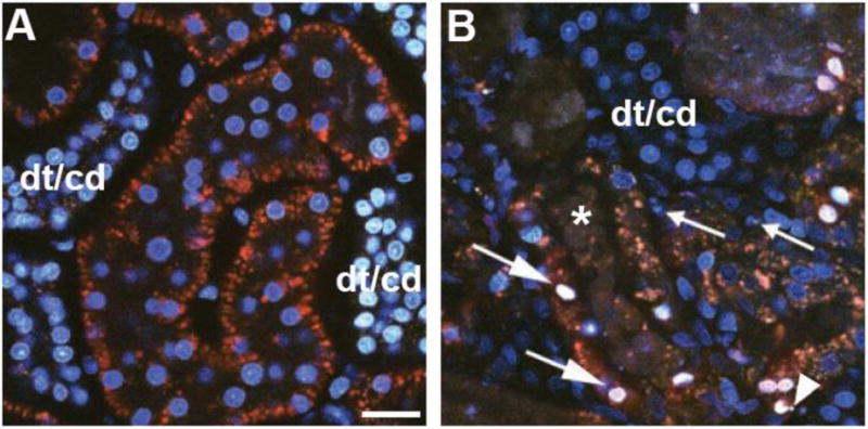
Quantifying apoptosis and necrosis. Apoptosis and necrosis can be assessed using cell permeant and impermeant nuclear dyes. Panel A shows a micrograph from an untreated rat with accumulation of the nuclear dye Hoechst 33342 (cyan) and exclusion of propidium iodide. Note the greater accumulation of Hoechst within distal tubule/collecting duct (dt/cd) cells at the left and right edge of the image. Panel B shows a micrograph from a rat that underwent ischemia and reperfusion. Apoptosis is detected by the hallmark signs of nuclear fragmentation (arrowhead) and condensation (small arrows). An influx of propidium iodide, normally cell impermeant, occurs when cell surface membranes are compromised following necrosis. The large arrows show colocalization of propidium iodide (red) with Hoechst 33342 (cyan) that gives a characteristic white appearance to the nuclei when overlaid. Heterogeneity in peritubular blood flow can alter delivery of the two dyes causing patchy distribution; note the cast material within the lumen of a Proximal Tubule (asterisk). (Bar= 20μm).

4.1

Administer a mixture of the two dyes in 0.9% normal saline intravenously and allow approximately 5-10 minutes for distribution and cellular accumulation to occur. Analysis can be done on single planes taken no deeper than 20μm into tissue, or on a reconstructed 3D volume no deeper than 20μm in depth. In normal tissue the broad emission spectra of the Hoecsts 33342 will stain nuclei under multi-photon illumination a cyan color. Cells positive for apoptosis will appear a brighter cyan color with condensed material at the nuclear margins. Necrotic cells that incorporate propidium iodide (red) will have a white appearance as the red stain from the proidium iodide mixes with the cyan from the Hoechst 33342. Hoechst does label different tubular epithelial cells at different intensities. Nuclei in distal tubules and collecting ducts will be brighter than those in proximal tubules. Despite this, necrotic and apoptotic nuclei within the same tubular population will be markedly brighter than those in viable cells.

4.2

A percentage of apoptotic and/or necrotic cells to the total number of cells can be made by cell counting.

5). Renal blood flow dynamics in normal and disease models

Materials

150 kDa Dextran, Hoechst 33342.

Ischemic injury induces multi-staged injury to the kidneys; the initial effects of ischemia are exacerbated by the flood of free radicals generated upon return of blood flow and oxygen. Intravital MPM reveals a heterogeneous landscape of normal and reduced red blood cell flow within the peritubular vasculature and glomerular capillary loops. This is caused by vasoconstriction and activated white blood cells rolling or adhering within the vessels causing focal obstruction. The use of a large molecular weight dextran in conjunction with the nuclear dye Hoechst 33342 allows for simple assessment of red blood cell (RBC) flow rates and the degree of white blood cell rolling and attachment [13]. Infusion of a large molecular weight dextran will fill in the circulating plasma and cause the RBC’s to appear in silhouette. In a typical mutli-photon laser scanning microscope system image acquisition occurs much slower than RBC flow, causing a motion artifact that makes them appear as streaks. This motion artifact can be exploited to determine RBC velocity based on the slope of the streaks as they flow through the peritubular vessels; a more shallow horizontal angle corresponds to a faster moving RBC[14, 15]. See figures 5 and 6.

Figure 5.

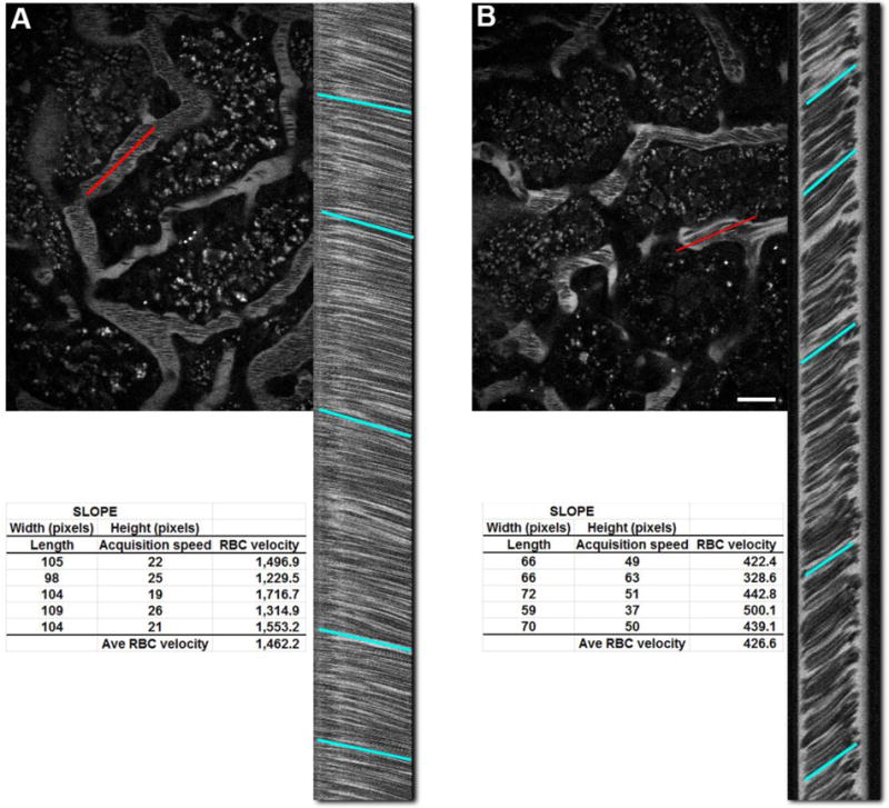
Determination of red blood cell flow rates. Red Blood Cell (RBCs) velocity can be calculated by exploiting a motion artifact during image acquisition. Images in laser scanning mutli-photon microscope are generated by scanning an area in a left to right raster scan, top to bottom. The prolonged acquistion time (typically 1 second) causes moving RBCs to appear as streaks as they move along the peritubular vasculature. Panel A shows an image from an untreated rat with a highlighted vessel (red line) and the corresponding linescan on the right side. The red line corresponds to the region of interest where the microscope scanned it 1,000 times and stacked the lines top to bottom to generate the linescan; time in the Y-axis and distance in the X-axis. Drawing a line to approximate the slope of the lines and applying the formula below gives RBC velocity:

RBC velocity = (pixel width of line × pixel size)/(pixel height of line × line acquisition speed in seconds.

Panel B shows an image taken from a rat after recovery from ischemic injury. Note the steeper slope associated with the linescan from the region selected (red line). The average RBC velocity for both images is shown at the bottom, generated by taking 5 samples along the length of the image. Small discrepancies in flow can be seen in the minute variation in the slope of the lines and their respective velocities. (Bar= 20μm).

Figure 6.

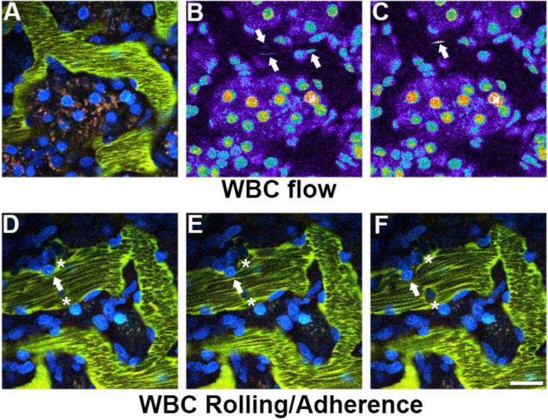
Quantifying white blood cell rolling and attachment. A measure of White Blood Cell (WBC) activation can be determined by characterizing their movement within the peritubular vessels. The nuclei of WBCs labeled with Hoechst 33342, shown in panels A, B, and C, appear as streaks (arrows) of varying intensity as they quickly move around with unlabeled circulating red blood cells. Once activated after ischemic injury and reperfusion (panels D, E and F), they are either adherent (asterisks), rolling along the vascular wall in the direction of flow (arrow) as seen in these successive images from a time series. (Bar= 20μm).

5.1

Infuse approximately 2.4 to 5.0 mg of a large 150kDa dextran intravenously and allow about 30 seconds for complete distribution; in injury or disease models this may take a few minutes. Use the microscope’s “linescan” setting to draw a line running parallel to a vessel along the middle to set up the region of interest. Acquire 1,000 lines to get a good sample size of the flowing RBCs. The resulting image is a tall column with a series of dark streaks running down the image.

5.2

When a line is drawn to approximate the slope of the streaks the height will give a time factor based on the acquisition speed and the width will give a size factor based on the objective used and zoom factor. Together these parameters can be used to accurately calculate RBC flow within the renal vasculature. Typically at least 5 lines are drawn to get an average of the RBC speed; this becomes more important in injury models as the slopes along the column tend to show greater variation. It is also important to note vessel diameter as smaller diameter vessels will have slower RBC velocities.

RBC velocity = (pixel width of line × pixel size)/(pixel height of line × line acquisition speed in seconds)

$$\text{Example}:\left(43\times 0.414\mu \mathrm{m}\right)/\left(11\times 0.002\text{seconds}\right)=809\mu \mathrm{m}/\text{second}$$

5.3

White Blood Cells (WBC) readily take up the nuclear dye Hoechst 33342 making them distinguishable from RBC. In normal rat kidneys WBCs flow freely within the renal vasculature and their nuclei appear as elongated streak typically in only one frame of a time series. In disease or injury models some WBCs seen in movies are adhered and do not move between successive frames. Activated WBCs can also roll along the vasculature and can be followed between successive frames[13].

5.4

To assess these parameters in the live rat, focus the objective on a region just below the capsule where the peritubular vasculature is clearly visible. Many microscope systems acquire images at approximately one frame per second when using the standard scanning mirrors to collect a standard 512 × 512 pixel image. Set up a time series to acquire a minimum of 30 frames.

5.5

To assist in quantifying the fast moving non-adhered white cells, break up the 512 × 512 image into four 256 × 256 quadrants and count the nuclear streaks (appearing in the blue channel) within the vasculature. The large molecular weight Fluorescein or Texas Red dextran will help determine the boundary of the vasculature. Counting the adhered and rolling WBC is much easier as they appear in subsequent frames. We score a cell as being adherent if it does not move for at least 4 frames (seconds). White blood cells that roll along the vascular wall for at least 4 frames prior to any dislodging are counted as rolling WBCs. To present these data, multiply these values by a factor, based on acquisition time, to convert them to occurrences per minute.

6). Vascular permeability

Vascular permeability: scoring with a large fluorescent dextran and fluorescent albumin.

Materials

150kDa dextran (Fluorescein conjugated), Texas Red rat serum albumin.

The integrity of the renal vasculature can be focally compromised during disease or injury causing larger molecular weight molecules such as 150kDa labeled dextrans, normally well retained within the microvasculature, to leak into the interstitial space. We assess permeability based on a scoring system between 0 and 3 with increasing numerical values corresponding to greater vascular leak. A score of zero indicates no material has leaked into the interstitial space. A score of one indicates there is a small amount of the material in the interstitial space in a minority of the image. A score of two indicates material has leaked into the interstitial space in the majority of the images. A score of three is given when enough material has leaked into the interstitial space that the intensity closely matches the intensity in the circulating plasma indicating severe leakage. The best area to focus on for this study is the region just below the capsule showing the basolateral side of the proximal tubules without showing the tubular lumen. This area will expose a large area of interstitial space. Of the two compounds utilized in this protocol the large 150kDa dextran is perhaps the better marker since this compound does not leak into the interstitial space under physiologic conditions [11]. See figure 7.

Figure 7.

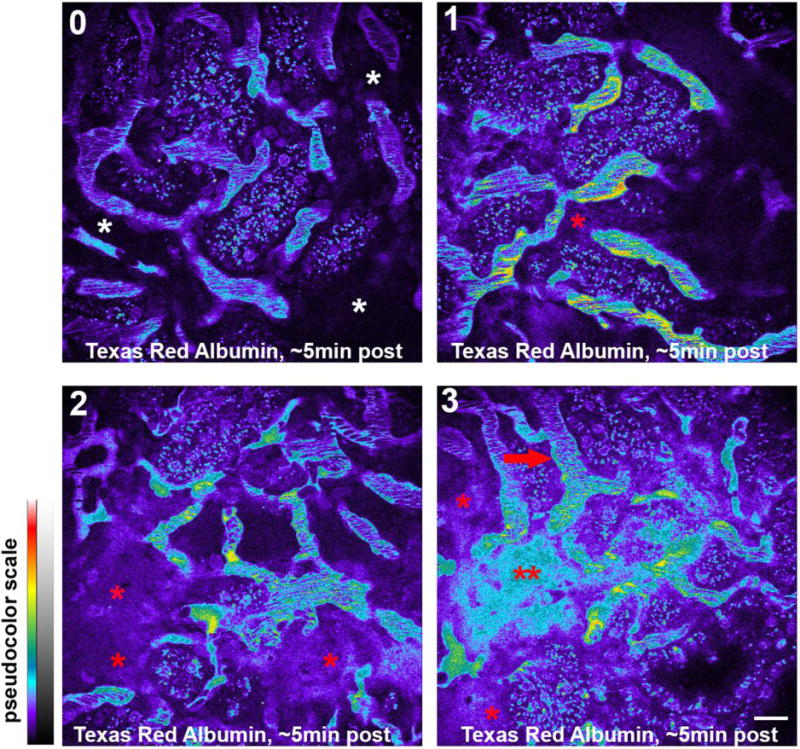
Quantifying vascular permeability. Leakage of large molecular weight compounds into the interstitial space can be scored to semi-quantify the severity of vascular leak. In this set of photomicrographs the leakage score is scored 0 to 3 indicated at the upper left. Tissue with a score of zero shows no leakage of compound into the interstitial space (white asterisks). Tissue with a score of one shows some leakage (red asterisk) into a small portion of the image. Tissue with a score of two shows leakage into a majority of the tissue (red asterisks). Tissues with a score of 3 have damage to the vasculature severe enough to cause extensive leakage where the intensity in the interstitial space (double red asterisks) closely approximates the intensity within the plasma (red arrow). (Bar= 20μm).

6.1

Select ten different random fields and mark them with the motorized stage on your microscope system. Infuse in ~2.5 to 5.0mg of a 150kDa fluorescein dextran and 3-4 mg of a Texas Red labeled albumin, being careful not to saturate the plasma intensity. Allow five minutes for complete systemic distribution.

6.2

Acquire images of the ten selected fields at 5, 15, and 30 minutes post infusion; this will allow visualization of progression within the same area. Try to closely match the focal plane for each region between the successive time points.

6.3

Score the images based on the aforementioned parameters. Statistical analysis of the scores can then be performed using any standard spreadsheet or statistical software package.

7). Glomerular Permeablity

Materials

Texas Red Albumin, large molecular weight dextrans, fluorescein-Inulin (freely filtered).

Traditional methods to assess glomerular permeability are based on methods such as micropuncture, which directly samples the filtrate with the tubular lumen and compares the concentration of the labeled compound to that found in the circulating plasma. A second method, fractional clearance, relies on the infusion, or constant infusion (for small molecular weight materials), of a labeled compound, collecting the urine and ratioing urinary concentration to that found within the plasma. The drawback to these two methods, particularly fractional clearance, is the underestimation of the filtered material (and hence a lower glomerular sieving coefficient) because these methods do not account for loss of material due to tubular reabsorption via fluid phase or receptor mediated endocytosis [4–9]. See figure 8.

Figure 8.

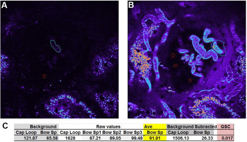
Determining glomerular permeability. Glomerular permeability for fluorescent compounds can be determined in Munich Wistar rats which have surface glomeruli. Calculating the glomerular permeability of a compound, the glomerular sieving coefficient (GSC), is done by first acquiring 3D volumes of glomeruli prior to infusion of any fluorescent compound. Panel A shows a glomerulus in the center with a capillary loop (cyan region) and the Bowman’s space (red region) outlined to determine background values; shown in panel C, left. The corresponding image in panel B, taken approximately 30 minutes after infusion of Texas Red conjugated Rat Serum Albumin (TR-RSA), shows a highlighted capillary loop with the highest plasma intensity (cyan region) and 3 regions within the Bowman’s space (red regions). The values for the Bowman’s space are averaged (panel C, yellow highlight) and the thresholded plasma intensity showing the brightest pixels, are reported as Raw values. The background values are then subtracted from the Raw values to determine the background corrected values which are then ratioed (Bowman’s space/Capillary loop) to determine the GSC. Here, a value of 0.017 (1.7%) is derived; note the bright accumulation of TR-RSA in the proximal tubules in the bottom and left side of the image that corroborates glomerular filtration and reclamation by the proximal tubule. (Bar= 20μm).

7.1

Scan the surface of the kidney of a Munich Wistar Frömter or Simonsen strain of rat with a low power immersion objective (a 20× W will work well) and mark the glomeruli on the system’s motorized stage.

7.2

Take 3D volumes of the glomeruli before infusing any fluorescent probe. These will be your background images. Insure you are using the full dynamic range of the system’s detectors, particularly the offset or black level. Every system features a palette warning the user if the pixels within an image are saturated (typically red) or at zero (typically blue or green). For background images, it is essential that only a few random pixels appear at zero; carefully adjust the black level to show this. When the black level is adjusted so that the Bowman’s space within a glomerulus is all zero (in an effort to totally eliminate background) there will be a marked loss in detector sensitivity and faint material within the Bowman’s capsule will not be detected [16, 17].

7.3

Focus in on a non-glomerular superficial blood vessel, the larger the better. Slowly infuse in the labeled compound via an indwelling i.v. line, allow time for distribution between pushes to assure the plasma levels of the compound will not saturate the detectors. Saturation will end the experiment.

7.4

Allow five to ten minutes for systemic distribution of material to reach equilibrium. Return to the glomeruli marked on the motorized stage and take 3D volumes of each.

7.5

For analysis, select the matching focal planes for the background 3D volume and post infusion 3D volume. These focal planes should be close to the surface showing a few capillary loops and an abundance of Bowman’s space. Superficial planes are chosen because of the high degree of light scatter that occurs at deeper focal depth [7]. In the background image draw a region to encompass a region of capillary loops (use a pseudocolor palette in your image analysis software to visualize this in background images) and a region within the Bowman’s space and note the values. For the post infusion image draw at least three regions within the Bowman’s space and average those values to report the intensity within the Bowman’s space. Choose the brightest capillary loop and draw a region around the brightest area; the region does not have to perfectly encompass the capillary loop. Next, using the threshold function, select the brightest area within the capillary loop (usually bordering the vessel wall), this should exclude the RBCs and areas between the RBCs. Make sure your software takes the intensity for the thresholded values within the region when noting these values.

7.6

Calculating glomerular permeability, known as the Glomerular Sieving Coefficient (GSC), for a compound is done as follows:

1. Raw Bowman’s Space average intensity (average of 3 regions) – background Bowman’s space value = Corrected Bowman’s space intensity.

2. Raw thresholded capillary loop intensity – background capillary loop intensity = Corrected capillary loop intensity

3. GSC=Corrected Bowmans’ Space intensity/Corrected capillary loop intensity. This value should be between zero (where no material filters into the Bowman’s space) and one (where a material freely filters into the Bowman’s space).

Note: Calculating GSC values for a large molecular weight compounds can be done using a single bolus injection. Calculating GSC values for a freely filtered or very small molecular weight compounds must be done under continuous infusion conditions. The rapidly falling plasma levels and rising Bowman’s space values can lead to reporting GSC values far in excess of one [18].

8). Differences between qualitative and intensity based quantitative analysis. The relevance of Offset in quantitative/ratiometric imaging

Data from all of the aforementioned examples of intravital MPM studies can be characterized into two broad categories. The first category is rooted in the characterization of morphology such as colocalizing fluorescent compounds to labeled organelles, changes in cellular and subcellular structures, and movement of an object across a defined space, such as RBC flow. The second category relies on the measurement of the fluorescence intensity of labeled compounds. This type of analysis encompasses physiologic parameters such as glomerular permeability of fluorescent compounds, and the degree to which a fluorescent compound accumulates within a cell or compartment. In the former category, instrument settings (particularly detector gain and offset) used in image acquisition have more flexibility since the ultimate goal is to best capture a shape or structure and note differences. Analysis of quantitative intensity-based data, however, obligates stringent attention to how instrument parameters and sensitivity are set to fully utilize the dynamic range of the system [16, 17]. As an example, the ratiometric intensities of the same compound within two compartments (low value compartment/high value compartment) can vary by orders of magnitude if the settings are incorrect. This is especially true of compounds with low permeability where the sensitivity of the microscope must be set correctly to capture the low intensity values found in the Bowman’s space. To utilize the full dynamic range of the detectors in your system it is crucial that offset, or black level settings, is set so that only a few pixels in the image randomly flash as having values of zero[16, 17]. Each microscope system has a palette that allows the user to determine if pixels within an image are saturated or if they display a value of zero. When taking background images it is intuitive to set the black level to have your area of interest at zero. In theory this would facilitate quantitation by removing the need for background subtraction. However in actuality, setting pixels to zero decreases sensitivity and compromises the detector’s ability to detect low intensity values[19, 20]. We conducted an extensive in vitro and in vivo study on this phenomenon and demonstrated a continued reduction in detector sensitivity as more and more pixels are set to zero. This decrease in sensitivity is initially linear when black level is adjusted to produces a moderate number of pixels at zero. As the number of pixels at zero increases, the decrease in sensitivity becomes exponential [17]. This results in erroneous data and incorrect conclusions [16, 19, 20]. See figure 9.

Figure 9.

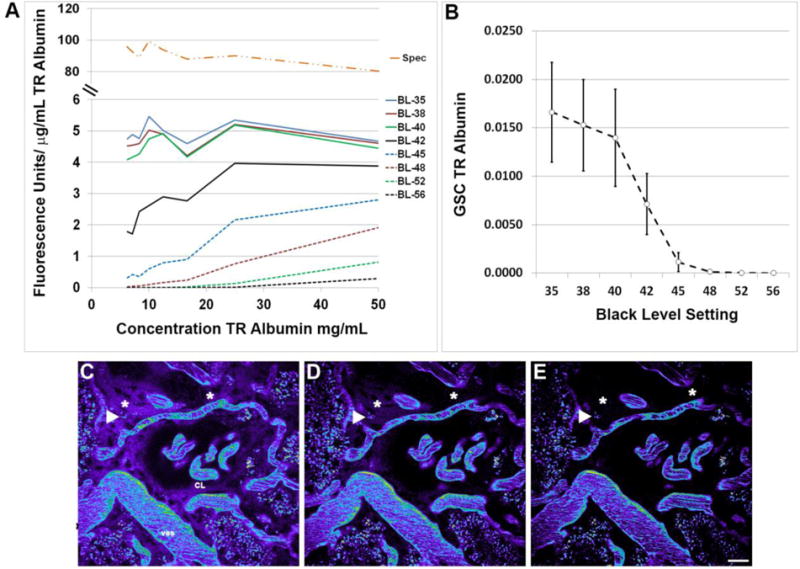
Setting low intensity value detector sensitivity. The black level or detector offset determines the sensitivity of the photo-multiplier tubes used in image acquisition. The graph in panel A shows the background subtracted fluorescence units acquired divided by the concentration of Texas Red rat serum albumin in both the multi-photon microscope (in vitro, BL-35 through BL-56) and the spectrophotometer (Spec). As the black level is increased (35 through 56) there is an increase in the number of low intensity pixels in an image that report a value of zero, hence the decrease in the sensitivity value (FU/μg/mL). The linearity in the sensitivity value seen across the range of concentrations studied should remain constant if there is no loss in sensitivity; note the linearity for the Spec and BL-35 through BL-40 and the progressive loss in linearity for BL-42 through BL-56. Examining the same phenomenon in vivo, by looking at the glomerular sieving coefficient of TR albumin, a decrease was seen in the GSC as the low intensity values within the Bowman’s space (see figure 9) became undetectable while the higher intensity values within the plasma were unaffected (panel B). Panels C, D and E show images from BL-38, BL-45, and BL-56; respectively. Here the high intensity structures such as the plasma within the capillary loops (CL), vessels (ves) and the accumulation at the arrowhead remain unchanged. The accumulation of TR albumin showing moderate intensity within the interstitial space (asterisks, 30 minutes post infusion all images) shows that even these values will eventually become undetectable if the detector offset is improperly set. (Bar= 20μm).

9). Future developments- Improving resolution at depth Far-Red dyes-our data

Present challenges in renal intravital MPM include the limited ability to penetrate opaque tissues like the liver and kidney. A tangible goal at present is to clearly image the bottom side of a surface glomerulus in the kidney and delineate the afferent and efferent arterioles (~100μm in depth). The use of far red-shifted emitting fluorophores and red-shifted excitation wavelengths (both of which scatter less), objectives and immersion media better suited for specific tissues (matching refractive indices), and engineering to place detectors in the closest proximity to the sample present very feasible starting points. Adaptive optics will also likely increase imaging depth. Another advantage to far red imaging is the increase in the usable dynamic range of the detector. The autofluorescent signal associated with the lysosomes of proximal tubules must be quantified and subtracted when quantifying accumulation of fluorescent compounds therein. On average the red and green signal emanating from autofluorescence consumes approximately 30 and 23% of the lower dynamic range in those images, respectively. A novel alternative made possible through the development of newer far-red dyes, excitable by multi-photon illumination, is to use a far-red channel. In preliminary studies, the slight lysosomal autofluorescence associated with the far-red channel (650nm-750nm emission) occupies approximately 6% of the lower dynamic range. See figure 10.

Figure 10.

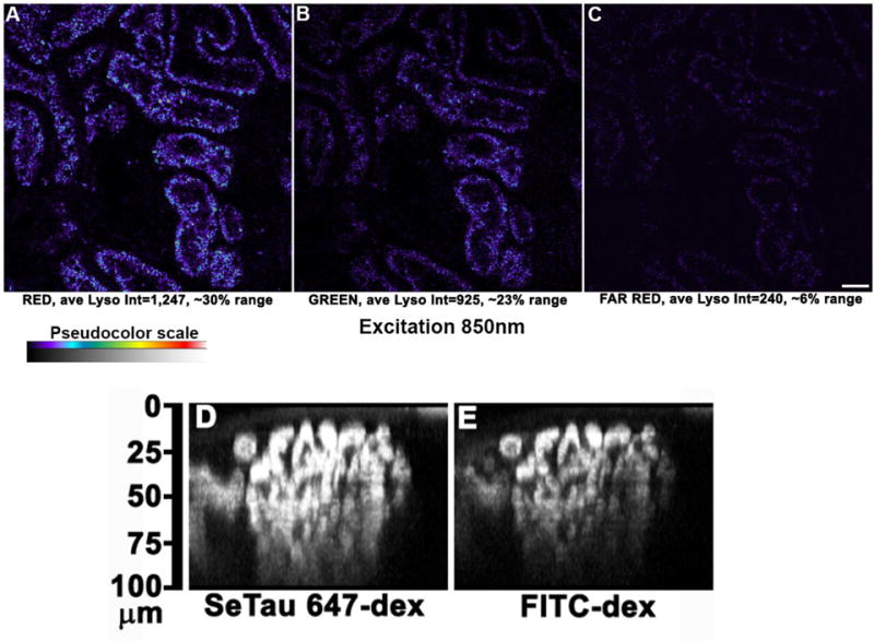
Far red dyes increase usable dynamic range and optical penetration. Images taken of the live kidney surface using an excitation wavelength of 850nm (versus the standard 800nm) show the signal intensity of autofluorescence for each channel, Red signal (A), Green signal (B), and Far Red signal (C) and the respective amount of detector range occupied by autofluorescence on the lower end of the detector range. Utilizing red-shifted fluorophores also allows deeper imaging into tissue. Large molecular weight dextrans conjugated to either a far red dye SeTau 647 or fluorescein are shown as they circulate within a glomerulus in an orthogonal X-Z reconstruction; panels D and E respectively. These images demonstrate the principle that red-shifted light is less susceptible to scatter and allows for deeper imaging in more opaque tissues. (Bar= 20μm).

In summary, intravital MPM can serve as an invaluable tool to enhance the research objectives of many laboratories studying physiology in the kidney or any organ that is accessible to exposure and placement for intravital MPM microscopy. Table one lists some of the processes that can be quantified. In particular, the ability to determine, in the same nephron, the role of the glomerulus and PT function has been an exciting development.

Table 1.

Dynamic Event	Sub-category	Author/Publication
Cellular Labeling and Uptake	Epithelial cell Endothelial cell Glomerulus Fluorescent proteins Uptake site (apical vs basolateral) Cell Volume, number, distribution	Sandoval et al. [2], Sandoval/Molitoris [21] Sipos et al.[22], Kalakeche et al. [23] Dunn et al.[1], Sandoval/Molitoris [21] Kaverina et al. [24], Hackl et al.[25] Sutton et al. [26], Hackl et al.[25] Tanner et al.[27], Collett et al.[28] Horbelt et al.[29], Tanner et al.[30], Hato et al.[31] Hackl et al. [25], Hato et al. [32]
Cellular Distriubtion	Site specific-organelle accumulation Cytosolic accumulation	Dunn et al.[1], Sandoval/Molitoris[21], Hall et al. [33] Sandoval/Molitoris [21], Molitoris et al.[34]
Cell Function	Endocytosis-Quantitative analysis Intracellular trafficking Transcytosis Renin secretion Signaling	Sandoval/Molitoris [12], Wagner et al. [8] Sandoval et al. [2], Sandoval et al. [7] Wagner et al. [8, 35] Sandoval et al. [7], Russo et al. [5] Toma et al [36], Sipos et al, [22] Kalakeche et al. [23]; El-Achkar/Dagher [37]
Glomerular	Size/volume Permability Fibrosis/sclerosis snGFR Macula Densa	Endres et al [38] Russo et al. [5, 6]; Sandoval et al [7, 17] Sandoval/Molitoris, [16]; Tanner [39, 40], Peti-Peterdi [41] Nakano et al. [18]; Schieβl/Castrop [19] Peti-Peterdi [42] Kang et al. [43] Sipos et al. [22]
Microvasculature	Blood flow rate Endothelial permeability White Blood Cell dynamics White Blood Cell tissue invasion Vasoconstriction	Sharfuddin et al. [13], Ferrell et al. [44]; Endres et al. [38] Sutton et al. [26], McCurley et al. [11] Sharfuddin et al. [13] Melican et al. [45] Mansson et al. [46, 47]
Epithelial Cell	Cell injury in necrosis/apoptosis Surface membrane blebbing Tubular flow	Dunn et al. [1], Kelly et al. [48] Tanner et al. [27] Kang et al. [43]; Carisoza-Gaytan et al. [49]

Highlights.

1. The ability to observe structure function relationships directly in a dynamic setting with 4D (time) imaging.

2. The ability to quantify physiologic parameters like capillary RBC flow and velocity directly and observe the effect of acute and chronic diseases on capillary flow. One can also follow WBC flow, rolling and adhesion.

3. The ability to quantify glomerular permeability under physiologic and disease states.

4. The ability to quantify proximal tubule cell uptake via endocytosis and also transcytosis of different molecules.

5. The ability to quantify apoptosis and necrosis and relate this to capillary flow in the area of interest.

References

- 1.Dunn KW, et al. Functional studies of the kidney of living animals using multicolor two-photon microscopy. Am J Physiol Cell Physiol. 2002;283(3):C905–16. doi: 10.1152/ajpcell.00159.2002. [DOI] [PubMed] [Google Scholar]
- 2.Sandoval RM, et al. Uptake and trafficking of fluorescent conjugates of folic acid in intact kidney determined using intravital two-photon microscopy. Am J Physiol Cell Physiol. 2004;287(2):C517–26. doi: 10.1152/ajpcell.00006.2004. [DOI] [PubMed] [Google Scholar]
- 3.Dickson LE, et al. The proximal tubule and albuminuria: really! J Am Soc Nephrol. 2014;25(3):443–53. doi: 10.1681/ASN.2013090950. [DOI] [PMC free article] [PubMed] [Google Scholar]
- 4.Russo LM, et al. Controversies in nephrology: response to ‘renal albumin handling, facts, and artifacts’. Kidney Int. 2007;72(10):1195–7. doi: 10.1038/sj.ki.5002528. [DOI] [PubMed] [Google Scholar]
- 5.Russo LM, et al. Impaired tubular uptake explains albuminuria in early diabetic nephropathy. J Am Soc Nephrol. 2009;20(3):489–94. doi: 10.1681/ASN.2008050503. [DOI] [PMC free article] [PubMed] [Google Scholar]
- 6.Russo LM, et al. The normal kidney filters nephrotic levels of albumin retrieved by proximal tubule cells: retrieval is disrupted in nephrotic states. Kidney Int. 2007;71(6):504–13. doi: 10.1038/sj.ki.5002041. [DOI] [PubMed] [Google Scholar]
- 7.Sandoval RM, et al. Multiple factors influence glomerular albumin permeability in rats. J Am Soc Nephrol. 2012;23(3):447–57. doi: 10.1681/ASN.2011070666. [DOI] [PMC free article] [PubMed] [Google Scholar]
- 8.Wagner MC, et al. Proximal Tubules Have the Capacity to Regulate Uptake of Albumin. J Am Soc Nephrol. 2016;27(2):482–94. doi: 10.1681/ASN.2014111107. [DOI] [PMC free article] [PubMed] [Google Scholar]
- 9.Sandoval RM, Molitoris BA. Quantifying glomerular permeability of fluorescent macromolecules using 2-photon microscopy in Munich Wistar rats. J Vis Exp. 201374 doi: 10.3791/50052. [DOI] [PMC free article] [PubMed] [Google Scholar]
- 10.Wang E, et al. Rapid diagnosis and quantification of acute kidney injury using fluorescent ratio-metric determination of glomerular filtration rate in the rat. Am J Physiol Renal Physiol. 2010;299(5):F1048–55. doi: 10.1152/ajprenal.00691.2009. [DOI] [PMC free article] [PubMed] [Google Scholar]
- 11.McCurley A, et al. Inhibition of alphavbeta5 Integrin Attenuates Vascular Permeability and Protects against Renal Ischemia-Reperfusion Injury. J Am Soc Nephrol. 2017 doi: 10.1681/ASN.2016020200. [DOI] [PMC free article] [PubMed] [Google Scholar]
- 12.Sandoval RM, Molitoris BA. Quantifying endocytosis in vivo using intravital two-photon microscopy. Methods Mol Biol. 2008;440:389–402. doi: 10.1007/978-1-59745-178-9_28. [DOI] [PubMed] [Google Scholar]
- 13.Sharfuddin AA, et al. Soluble thrombomodulin protects ischemic kidneys. J Am Soc Nephrol. 2009;20(3):524–34. doi: 10.1681/ASN.2008060593. [DOI] [PMC free article] [PubMed] [Google Scholar]
- 14.Choong FX, et al. Multiphoton microscopy applied for real-time intravital imaging of bacterial infections in vivo. Methods Enzymol. 2012;506:35–61. doi: 10.1016/B978-0-12-391856-7.00027-5. [DOI] [PMC free article] [PubMed] [Google Scholar]
- 15.Molitoris BA, Sandoval RM. Intravital multiphoton microscopy of dynamic renal processes. Am J Physiol Renal Physiol. 2005;288(6):F1084–9. doi: 10.1152/ajprenal.00473.2004. [DOI] [PubMed] [Google Scholar]
- 16.Sandoval RM, Molitoris BA. Letter to the editor: “Quantifying albumin permeability with multiphoton microscopy: why the difference?”. Am J Physiol Renal Physiol. 2014;306(9):F1098–100. doi: 10.1152/ajprenal.00652.2013. [DOI] [PMC free article] [PubMed] [Google Scholar]
- 17.Sandoval RM, Wang E, Molitoris BA. Finding the bottom and using it: Offsets and sensitivity in the detection of low intensity values in vivo with 2-photon microscopy. Intravital. 2014;2(1) doi: 10.4161/intv.23674. [DOI] [PMC free article] [PubMed] [Google Scholar]
- 18.Nakano D, et al. Multiphoton imaging of the glomerular permeability of angiotensinogen. J Am Soc Nephrol. 2012;23(11):1847–56. doi: 10.1681/ASN.2012010078. [DOI] [PMC free article] [PubMed] [Google Scholar]
- 19.Schiessl IM, Castrop H. Angiotensin II AT2 receptor activation attenuates AT1 receptor-induced increases in the glomerular filtration of albumin: a multiphoton microscopy study. Am J Physiol Renal Physiol. 2013;305(8):F1189–200. doi: 10.1152/ajprenal.00377.2013. [DOI] [PubMed] [Google Scholar]
- 20.Schiessl IM, Kattler V, Castrop H. In vivo visualization of the antialbuminuric effects of the angiotensin-converting enzyme inhibitor enalapril. J Pharmacol Exp Ther. 2015;353(2):299–306. doi: 10.1124/jpet.114.222125. [DOI] [PubMed] [Google Scholar]
- 21.Molitoris BA, Sandoval RM. Pharmacophotonics: utilizing multi-photon microscopy to quantify drug delivery and intracellular trafficking in the kidney. Adv Drug Deliv Rev. 2006;58(7):809–23. doi: 10.1016/j.addr.2006.07.017. [DOI] [PubMed] [Google Scholar]
- 22.Sipos A, et al. Advances in renal (patho)physiology using multiphoton microscopy. Kidney Int. 2007;72(10):1188–91. doi: 10.1038/sj.ki.5002461. [DOI] [PMC free article] [PubMed] [Google Scholar]
- 23.Kalakeche R, et al. Endotoxin uptake by S1 proximal tubular segment causes oxidative stress in the downstream S2 segment. J Am Soc Nephrol. 2011;22(8):1505–16. doi: 10.1681/ASN.2011020203. [DOI] [PMC free article] [PubMed] [Google Scholar]
- 24.Kaverina NV, et al. Tracking the stochastic fate of cells of the renin lineage after podocyte depletion using multicolor reporters and intravital imaging. PLoS One. 2017;12(3):e0173891. doi: 10.1371/journal.pone.0173891. [DOI] [PMC free article] [PubMed] [Google Scholar]
- 25.Hackl MJ, et al. Tracking the fate of glomerular epithelial cells in vivo using serial multiphoton imaging in new mouse models with fluorescent lineage tags. Nat Med. 2013;19(12):1661–6. doi: 10.1038/nm.3405. [DOI] [PMC free article] [PubMed] [Google Scholar]
- 26.Sutton TA, et al. Injury of the renal microvascular endothelium alters barrier function after ischemia. Am J Physiol Renal Physiol. 2003;285(2):F191–8. doi: 10.1152/ajprenal.00042.2003. [DOI] [PubMed] [Google Scholar]
- 27.Tanner GA, et al. Micropuncture gene delivery and intravital two-photon visualization of protein expression in rat kidney. Am J Physiol Renal Physiol. 2005;289(3):F638–43. doi: 10.1152/ajprenal.00059.2005. [DOI] [PubMed] [Google Scholar]
- 28.Collett JA, et al. Hydrodynamic Isotonic Fluid Delivery Ameliorates Moderate-to-Severe Ischemia-Reperfusion Injury in Rat Kidneys. J Am Soc Nephrol. 2017 doi: 10.1681/ASN.2016040404. [DOI] [PMC free article] [PubMed] [Google Scholar]
- 29.Horbelt M, et al. Organic cation transport in the rat kidney in vivo visualized by time-resolved two-photon microscopy. Kidney Int. 2007;72(4):422–9. doi: 10.1038/sj.ki.5002317. [DOI] [PubMed] [Google Scholar]
- 30.Tanner GA, Sandoval RM, Dunn KW. Two-photon in vivo microscopy of sulfonefluorescein secretion in normal and cystic rat kidneys. Am J Physiol Renal Physiol. 2004;286(1):F152–60. doi: 10.1152/ajprenal.00264.2003. [DOI] [PubMed] [Google Scholar]
- 31.Hato T, et al. Novel application of complementary imaging techniques to examine in vivo glucose metabolism in the kidney. Am J Physiol Renal Physiol. 2016;310(8):F717–F725. doi: 10.1152/ajprenal.00535.2015. [DOI] [PMC free article] [PubMed] [Google Scholar]
- 32.Hato T, et al. Two-Photon Intravital Fluorescence Lifetime Imaging of the Kidney Reveals Cell-Type Specific Metabolic Signatures. J Am Soc Nephrol. 2017 doi: 10.1681/ASN.2016101153. [DOI] [PMC free article] [PubMed] [Google Scholar]
- 33.Hall AM, et al. In vivo multiphoton imaging of mitochondrial structure and function during acute kidney injury. Kidney Int. 2013;83(1):72–83. doi: 10.1038/ki.2012.328. [DOI] [PMC free article] [PubMed] [Google Scholar]
- 34.Molitoris BA, et al. siRNA targeted to p53 attenuates ischemic and cisplatin-induced acute kidney injury. J Am Soc Nephrol. 2009;20(8):1754–64. doi: 10.1681/ASN.2008111204. [DOI] [PMC free article] [PubMed] [Google Scholar]
- 35.Wagner MC, et al. Mechanism of increased clearance of glycated albumin by proximal tubule cells. Am J Physiol Renal Physiol. 2016;310(10):F1089–102. doi: 10.1152/ajprenal.00605.2015. [DOI] [PMC free article] [PubMed] [Google Scholar]
- 36.Toma I, Kang JJ, Peti-Peterdi J. Imaging renin content and release in the living kidney. Nephron Physiol. 2006;103(2):71–4. doi: 10.1159/000090622. [DOI] [PubMed] [Google Scholar]
- 37.El-Achkar TM, Dagher PC. Tubular cross talk in acute kidney injury: a story of sense and sensibility. Am J Physiol Renal Physiol. 2015;308(12):F1317–23. doi: 10.1152/ajprenal.00030.2015. [DOI] [PMC free article] [PubMed] [Google Scholar]
- 38.Endres BT, et al. Intravital Imaging of the Kidney in a Rat Model of Salt-Sensitive Hypertension. Am J Physiol Renal Physiol. 2017 doi: 10.1152/ajprenal.00466.2016. ajprenal 00466 2016. [DOI] [PMC free article] [PubMed] [Google Scholar]
- 39.Tanner GA. Glomerular sieving coefficient of serum albumin in the rat: a two-photon microscopy study. Am J Physiol Renal Physiol. 2009;296(6):F1258–65. doi: 10.1152/ajprenal.90638.2008. [DOI] [PubMed] [Google Scholar]
- 40.Tanner GA, et al. Glomerular permeability to macromolecules in the Necturus kidney. Am J Physiol Renal Physiol. 2009;296(6):F1269–78. doi: 10.1152/ajprenal.00371.2007. [DOI] [PubMed] [Google Scholar]
- 41.Peti-Peterdi J. Independent two-photon measurements of albumin GSC give low values. Am J Physiol Renal Physiol. 2009;296(6):F1255–7. doi: 10.1152/ajprenal.00144.2009. [DOI] [PMC free article] [PubMed] [Google Scholar]
- 42.Peti-Peterdi J. A practical new way to measure kidney fibrosis. Kidney Int. 2016;90(5):941–942. doi: 10.1016/j.kint.2016.07.036. [DOI] [PMC free article] [PubMed] [Google Scholar]
- 43.Kang JJ, et al. Quantitative imaging of basic functions in renal (patho)physiology. Am J Physiol Renal Physiol. 2006;291(2):F495–502. doi: 10.1152/ajprenal.00521.2005. [DOI] [PubMed] [Google Scholar]
- 44.Ferrell N, et al. Shear stress is normalized in glomerular capillaries following (5/6) nephrectomy. Am J Physiol Renal Physiol. 2015;308(6):F588–93. doi: 10.1152/ajprenal.00290.2014. [DOI] [PMC free article] [PubMed] [Google Scholar]
- 45.Melican K, et al. Bacterial infection-mediated mucosal signalling induces local renal ischaemia as a defence against sepsis. Cell Microbiol. 2008;10(10):1987–98. doi: 10.1111/j.1462-5822.2008.01182.x. [DOI] [PubMed] [Google Scholar]
- 46.Mansson LE, et al. Real-time studies of the progression of bacterial infections and immediate tissue responses in live animals. Cell Microbiol. 2007;9(2):413–24. doi: 10.1111/j.1462-5822.2006.00799.x. [DOI] [PubMed] [Google Scholar]
- 47.Mansson LE, et al. Progression of bacterial infections studied in real time–novel perspectives provided by multiphoton microscopy. Cell Microbiol. 2007;9(10):2334–43. doi: 10.1111/j.1462-5822.2007.01019.x. [DOI] [PubMed] [Google Scholar]
- 48.Kelly KJ, et al. A novel method to determine specificity and sensitivity of the TUNEL reaction in the quantitation of apoptosis. Am J Physiol Cell Physiol. 2003;284(5):C1309–18. doi: 10.1152/ajpcell.00353.2002. [DOI] [PubMed] [Google Scholar]
- 49.Carrisoza-Gaytan R, et al. Effects of biomechanical forces on signaling in the cortical collecting duct (CCD) Am J Physiol Renal Physiol. 2014;307(2):F195–204. doi: 10.1152/ajprenal.00634.2013. [DOI] [PMC free article] [PubMed] [Google Scholar]