Histological Validation of Diffusion MRI Fiber Orientation Distributions and Dispersion

Abstract

Diffusion magnetic resonance imaging (dMRI) is widely used to probe tissue microstructure, and is currently the only non-invasive way to measure the brain’s fiber architecture. While a large number of approaches to recover the intra-voxel fiber structure have been utilized in the scientific community, a direct, 3D, quantitative validation of these methods against relevant histological fiber geometries is lacking. In this study, we investigate how well different high angular resolution diffusion imaging (HARDI) models and reconstruction methods predict the ground-truth histologically defined fiber orientation distribution (FOD), as well as investigate their behavior over a range of physical and experimental conditions. The dMRI methods tested include constrained spherical deconvolution (CSD), Q-ball imaging (QBI), diffusion orientation transform (DOT), persistent angular structure (PAS), and neurite orientation dispersion and density imaging (NODDI) methods. Evaluation criteria focus on overall agreement in FOD shape, correct assessment of the number of fiber populations, and angular accuracy in orientation. In addition, we make comparisons of the histological orientation dispersion with the fiber spread determined from the dMRI methods. As a general result, no HARDI method outperformed others in all quality criteria, with many showing tradeoffs in reconstruction accuracy. All reconstruction techniques describe the overall continuous angular structure of the histological FOD quite well, with good to moderate correlation (median angular correlation coefficient > 0.70) in both single- and multiple-fiber voxels. However, no method is consistently successful at extracting discrete measures of the number and orientations of FOD peaks. The major inaccuracies of all techniques tend to be in extracting local maxima of the FOD, resulting in either false positive or false negative peaks. Median angular errors are ~10° for the primary fiber direction and ~20° for the secondary fiber, if present. For most methods, these results did not vary strongly over a wide range of acquisition parameters (number of diffusion weighting directions and b value). Regardless of acquisition parameters, all methods show improved successes at resolving multiple fiber compartments in a voxel when fiber populations cross at near-orthogonal angles, with no method adequately capturing low to moderate angle (<60 degrees) crossing fibers. Finally, most methods are limited in their ability to capture orientation dispersion, resulting in low to moderate, yet statistically significant, correlation with histologically-derived dispersion with both HARDI and NODDI methodologies. Together, these results provide quantitative measures of the reliability and limitations of dMRI reconstruction methods and can be used to identify relative advantages of competing approaches as well as potential strategies for improving accuracy.

1. Introduction

Diffusion magnetic resonance imaging (dMRI) has proven a valuable neuroscience tool due to its unique ability to provide information about tissue composition, microstructure, and structural connectivity of the brain non-invasively (Basser and Pierpaoli, 1996; Johansen-Berg and Behrens, 2014). In the white matter, the diffusion-driven displacements of water molecules are hindered by the organization of intra and extra-cellular tissue components (Beaulieu, 2002), making it possible to infer the distribution of neuronal fiber orientations in each voxel from a set of diffusion measurements, an object often referred to as the fiber orientation distribution (FOD). Fiber tractography can then be performed by following these fiber orientation estimates from voxel to voxel throughout the brain in order to reconstruct the structural connections between different brain areas (Mori et al., 1999; Mori and van Zijl, 2002).

There are a number of assumptions and uncertainties that can affect the ability of fiber tractography to faithfully represent the true axonal connections of the brain. The most obvious potential source of error is in the inference of fiber orientation in each MRI voxel (Jbabdi et al., 2015; Jones and Cercignani, 2010). The challenge here lies in the fact that axons have diameters in the micron range, while a typical MRI voxel can be on the order of millimeters and contain hundreds of thousands of axons (Aboitiz et al., 1992; Van Essen and Ugurbil, 2012) with a wide range of possible configurations, which makes the mapping from diffusion signal to axon orientation an ill-posed problem (where many patterns are likely to give rise to the same MRI measurement). In addition, the choice of dMRI reconstruction method in combination with experimental conditions, including the number of diffusion weighted images (DWIs) and the amount of diffusion weighting (the “b-value”), are expected to result in different inferences of the fiber geometry in each voxel. Because these estimates of fiber orientation form the input to nearly all fiber tracking algorithms, it is critical that the validity of experimentally estimated orientation information be checked and quantified against the true physical geometry of fibers under investigation.

Diffusion tensor imaging (DTI), the first reconstruction method to allow mapping of fiber orientations throughout the brain, models diffusion as a 3D Gaussian distribution (Basser et al., 1994). While the fiber orientation estimates from DTI have been validated in large coherent fiber bundles, a significant limitation of DTI is that it cannot adequately capture the underlying structure in voxels containing complex white matter architectures or multiple fiber populations. This “crossing fiber” problem has motivated the development of a large number of reconstruction methods which aim to resolve multiple fiber orientations and recover complex fiber configurations (Aganj et al., 2010; Anderson, 2005; Assaf and Basser, 2005; Canales-Rodriguez et al., 2010; Dell’acqua et al., 2010; Descoteaux et al., 2007; Jansons and Alexander, 2003; Ozarslan et al., 2006; Tournier et al., 2007; Tournier et al., 2004; Tuch, 2004; Wedeen et al., 2005). These algorithms, typically referred to as high angular resolution diffusion imaging (HARDI) methods, differ in a number of aspects, including acquisition requirements, fundamental assumptions on diffusion processes, and the representation of orientation information. Some techniques estimate the FOD directly, whereas others estimate a diffusion orientation distribution function (dODF) describing the probability of diffusion in a given direction, with the assumption that fiber orientations coincide with the peaks of the dODF. Finally, while some reconstruction methods do not explicitly model diffusion in white matter, others model distinct tissue compartments and fiber populations separately. For example, a common compartmental model, termed NODDI (neurite orientation dispersion and density imaging) (Zhang et al., 2012), utilizes a fiber orientation dispersion index (ODI) to characterize the geometrical angular variation of the fiber populations. Similarly, measures of dispersion can be extracted from the FOD and ODF directly (Dell’Acqua et al., 2013; Raffelt et al., 2012; Riffert et al., 2014) as a way to characterize the fiber geometry in a voxel. Due to the large number of reconstruction methods, and differences among them, a direct validation and comparison among techniques remains very difficult.

The validation method of choice for most reconstruction algorithms (Aganj et al., 2010; Canales-Rodriguez et al., 2009; Descoteaux et al., 2007; Ozarslan et al., 2006; Tournier et al., 2007; Tuch et al., 2002), or comparison of algorithms (Alexander, 2005; Daducci et al., 2014), is through numerical simulations. Simulations offer the versatility of assessing performance across a broad range of physical and experimental conditions. However, they rely on assumptions and approximations to generate the modeled dMRI signal that are likely to be over-simplifications of complex biological tissue. Physical phantoms add additional complexity and realism to the validation process by incorporating practical effects of image acquisition. Yet, these synthetic fiber-based (Farrher et al., 2012; Fieremans et al., 2008) and capillary-based (Lin et al., 2003; Yanasak and Allison, 2006) phantoms can still fail to replicate the biological characteristics of brain tissue, including membrane permeability, axon diameters, and the geometric complexity of the central nervous system. Finally, validation of orientation information has been performed by comparisons with the results of histological analysis (Choe et al., 2012; Gangolli et al., 2017; Leergaard et al., 2010; Seehaus et al., 2015). While offering exquisite detail of the tissue microstructure, these studies have been limited to two-dimensional analysis of tissue sections, restricting investigation to only those fibers oriented parallel to the plane of sectioning. Recently, several groups have explored the use of confocal microscopy (Jespersen et al., 2012; Schilling et al., 2016), optical coherence tomography (Wang et al., 2015), and polarized light imaging (Axer et al., 2016; Mollink et al., 2017) as a means of extracting the 3D histological FOD for direct comparison with dMRI. Despite these advances, most histological validation studies have studied only a few axonal tracts or MRI voxels, and none have investigated the performance of multiple reconstruction algorithms, nor studied the effect of varying acquisition parameters on their performance.

Thus, there is a need to characterize the distribution of neuronal fibers in 3D using histology and make direct comparisons to the corresponding dMRI estimated orientation distributions. With this in mind, the aim of this study is to determine how well different dMRI models and reconstruction methods predict the ground truth FODs, as well as investigate the effect of fiber geometry, b-value, and number of gradient directions on the accuracy of the reconstruction methods. This is done by extracting the ground truth FOD from 3D confocal data of ex vivo tissue followed by spatial registration of the dMRI data to the z-stacks to facilitate comparisons of the same tissue volume. The results of this study are measures of reliability and accuracy of competing intra-voxel fiber reconstruction methods, as well as highlights of the relative merits and limitations of state-of-the-art techniques for analysis of dMRI data.

2. Methods

2.1 MRI acquisition

All animal procedures were approved by the Vanderbilt University Animal Care and Use Committee. Diffusion MRI experiments were performed on three adult squirrel monkey brains that had been perfused with physiological saline followed by 4% paraformaldehyde. The brain was then immersed for 3 weeks in phosphate-buffered saline (PBS) medium with 1mM Gd-DTPA in order to reduce longitudinal relaxation time (D’Arceuil et al., 2007). The brain was placed in liquid Fomblin (California Vacuum Technology, CA) and scanned on a Varian 9.4 T, 21 cm bore magnet using a quadrature birdcage volume coil (inner diameter = 63 mm).

Diffusion data were acquired with a 3D spin-echo diffusion-weighted EPI sequence (TR = 410ms; TE = 41ms; NSHOTS = 4; NEX = 1; Partial Fourier k-space coverage = .75) at 300um isotropic resolution. Diffusion gradient pulse duration and separation were 8ms and 22ms, respectively, and the b-value was set to 6,000 s/mm2. This value was chosen due to the decreased diffusivity of ex vivo tissue, which is approximately a fourth of that in vivo (Dyrby et al., 2011; Schilling et al., 2017b), and is expected to closely replicate the signal attenuation profile for in vivo tissue with a b-value of approximately 1,500 s/mm2. A gradient table of 100 uniformly distributed directions (Caruyer et al., 2013) was used to acquired 100 diffusion-weighted volumes with four additional image volumes collected at b = 0. Unless otherwise noted, all analysis was performed on this dataset.

In order to assess the effects of diffusion weighting on reconstruction accuracy, the full diffusion acquisition was repeated with b-values of 3,000, 9,000, and 12,000 s/mm2, while keeping all other acquisition parameters (including diffusion times) constant.

2.2 Histological Procedures

Here, we aim to extract the histological FOD from 3D confocal z-stacks in areas equivalent to the size of an MRI voxel. To do this, we utilized an image processing technique, structure tensor analysis (Bigun and Granlund, 1987), which results in an orientation estimate for every pixel in the 3D z-stack that is occupied by a fiber.

Following the methodology described in (Schilling et al., 2016), histological procedures consisted of tissue sectioning and staining, confocal acquisition, and confocal pre-processing. After MR imaging, the brain was sectioned on a cryomicrotome at a thickness of 50um in the coronal plane. Using a Canon EOS20D (Lake Success, NY, USA) digital camera, the tissue block was digitally photographed prior to cutting every third section, resulting in a 3D “block-face” volume with a through-plane resolution of 150um. Tissue sections were mounted on glass slides and stained with the fluorescent lipophilic dye, “DiI” (1,1′-dioctadecyl-3,3,3′3′-tetramethylindocarbocyanine perchlorate) diluted in 100% ethanol at 0.25mg/mL.

Slides were imaged using an LSM 710 confocal microscope (Carl Zeiss, Inc. Thornwood, NY. USA). For all selected tissue slices, confocal acquisition consists of two protocols: [1] creating a 2D montage of the entire tissue section and [2] constructing a 3D high-resolution image in a selected region of interest. The 2D montage (Fig. 1A) consists of approximately 600–900 individual tiles acquired using a 10x oil objective at a resolution of 0.80μm², which are stitched together using Zeiss software, ZEN 2010. This 2D montage is used for image registration, and for localizing the 3D high-resolution region of interest. The 3D z-stack (Fig. 1B) was then collected using a 63x oil objective at a nominal resolution of 0.18μm×0.18μm×0.42μm, with an in-plane field of view of 900μm×900μm (equivalent to 9 MRI voxels). The through-plane resolution is the “optimal” slice-thickness, calculated from the LSM710 software based on a 1.0 Airy unit pinhole diameter and an excitation wavelength of 543nm.

Figure 1.

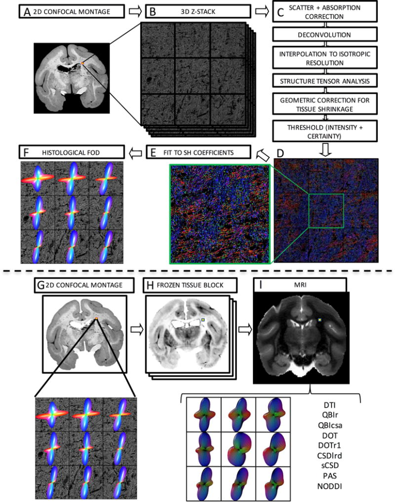
Histological procedures (top) and image registration (bottom). Confocal acquisition includes a 2D low-resolution montage (A) and a high-resolution 3D z-stack (B). Image pre-processing (C) comprises light scatter and absorption correction, deconvolution, and interpolation, followed by structure tensor analysis. This is followed by geometric correction for tissue shrinkage and thresholding fibers. This results in an orientation estimate for every pixel in the z-stack occupied by a fiber, here shown as an RGB color map (D) where red, green, and blue represent fiber oriented right/left, anterior/posterior, and superior/inferior. Zooming in on the center voxel shows crossing fibers oriented primarily left/right and superior/inferior. Fitting the orientation distribution to spherical harmonic coefficients (E) results in the histologically defined ground truth FODs, displayed as 3D glyphs (F). The registration procedure involves 2D registration of the 2D confocal montage (G) to the corresponding frozen tissue block (H) and subsequent 3D registration to the non-diffusion weighted image (I). From this, the signal corresponding to the high-resolution z-stack can be determined and processed using a chosen reconstruction method for direct voxel-wise comparison of histology and dMRI.

Four slices were randomly selected for each monkey (12 total slices) for confocal imaging. For each slice, multiple regions of interest were chosen to image (using the above protocol) in order to capture both voxels with coherent single fiber populations, as well as expected regions of crossing fibers. This was done using prior anatomical knowledge of squirrel monkey white matter bundles. For crossing fiber regions, sampling was continued until a sample size of at least N>10 was collected for each histogram bin of crossing angles, ranging from <30° to 90°, with a bin width of 10°.

During imaging, it was necessary to increase the laser output as deeper layers were imaged, due to increases in net light scatter and absorption at greater depths. The laser power was adjusted at approximately 5 different depths ranging from the coverslip to the end of the tissue, at each step ensuring that the image intensity covered the full 8-bit depth from 0–255 units. Stitching, again, was performed using ZEN 2010 software to create a single 3D z-stack. Finally, all confocal data were converted from the LSM file format to TIFF images and imported into MATLAB for further processing.

Prior to structure tensor analysis, four sources of anisotropy inherent to confocal microscopy must be accounted for (Fig. 1C). Three corrections were performed directly on the z-stack prior to structure tensor analysis, and the final correction performed post-analysis (see Section 2.3). First, as previously described, attenuation correction was performed during acquisition by increasing laser power for deeper tissue layers in order to generate a z-profile that has a relatively constant mean intensity in each x-y plane. The second source of anisotropy arises from the confocal microscope’s point spread function (PSF) (Pawley and Masters, 1996), which was corrected using the iterative Lucy-Richardson deconvolution algorithm (Biggs and Andrews, 1997) and a computed theoretical model of the microscope’s PSF (Pawley and Masters, 1996). Finally, cubic interpolation to isotropic resolution was performed to correct for the anisotropic acquisition resolution. This ensures that fibers oriented laterally in the image will contain an equivalent number of pixels per length as those oriented axially.

2.3 Histological FOD

Next, pixel-wise fiber orientations in the 3D z-stack were obtained via structure tensor analysis (Bigun and Granlund, 1987) (See Appendix A). After fiber orientations had been estimated, one final correction for anisotropy was performed. Tissue samples may shrink due to fixation and dehydration during the staining procedure (Wehrl et al., 2015; Williams et al., 1997), which could bias fiber orientation estimates. We use a thickness measurement before acquisition of each 3D z-stack to perform a geometric correction to the orientation estimation for every pixel in the image by assuming linear shrinkage in the through-plane (z) direction. Tissue thickness is calculated as the difference between the highest and lowest stage position where fluorescence is observed from each individual z-stack field of view. Pixel-wise structure tensor orientations are re-oriented based on the correction factor calculated from the measured thickness and expected thickness (50um). Once re-oriented, the results were thresholded using both image intensity and an orientation “certainty” value (see Appendix A) in order to exclude non-fiber areas and pixels where the orientation estimate is unreliable. This results in an orientation estimate for every pixel in our z-stack that is occupied by a fiber (Fig. 1D).

The histological FOD was then computed as the histogram of the extracted fiber orientations, and fit to high order (20) spherical harmonic coefficients (SH) (Fig. 1E). Throughout this paper, the FODs are displayed as 3D glyphs (Fig. 1F) in the same way that the MRI-FOD’s are typically displayed in literature.

2.4 Image Registration

In order to make quantitative comparisons of the histological FODs with estimates derived from MRI, the data must be aligned and oriented appropriately. A multi-step registration procedure (Choe et al., 2011) was used to align histology to MRI data. The first step is registration of the 2D confocal montage (Fig. 1G) to the corresponding block face image (Fig. 1H) using mutual information based 2D linear registration followed by 2D nonlinear registration using the adaptive bases algorithm (ABA) (Rohde et al., 2003). Next, all block face photographs were assembled into a 3D block volume, and registered to the MRI b=0 image (Fig. 1I) using a 3D affine transformation followed by 3D nonlinear registration with ABA. Given the location of the 3D z-stack in the 2D confocal montage, we can use the combined deformation fields to determine the MRI signal from the same tissue volume. The MRI signal of interest is analyzed in MRI native space using the chosen reconstruction method (Fig. 1I), and transformed to histological space in order to facilitate comparisons with the histological FOD. To do this, we implement the preservation of principle directions strategy (Alexander et al., 2001) that takes into account rotation, scaling, and shearing effects of the spatial transformations, and can be applied to any orientation distribution on a sphere (Hong et al., 2009). After these corrections, both the histological FOD and the MRI derived measure of interest (FOD or ODF, and derived metrics) are in histological space, and quantitative analysis can be performed. This multi-step registration procedure was validated in an earlier study (Choe et al., 2011), which showed that the accuracy of the overall registration was approximately one MRI voxel (~0.3mm) by comparing position errors between manually chosen landmarks in histological and MRI space. Further, the combination of registration and histological procedures (see Section 2.2) is similar to those utilized in (Schilling et al., 2016), which showed an angular accuracy of approximately 5°, or less, in single fiber regions when compared to manually defined ground truth fiber orientations.

2.5 MRI Reconstruction Methods

In this section, we give a brief description of the reconstruction models implemented in the study. Again, the focus is on those that attempt to describe the underlying fiber orientation information. Because of the large number of these techniques proposed in literature, the assessment presented in this work is not exhaustive, yet comprises some of the more commonly implemented reconstruction techniques. All MRI techniques resulting in a function over a sphere are represented as SH series, where the SH order is determined by the number of DWI’s utilized in calculation, up to a maximum of order 8 (Tournier et al., 2013). Unless otherwise noted, all reconstruction algorithms are implemented using the Matlab HARDI Toolbox (freely available at NeuroImageN.es) with default parameters.

DTI: the tensor models the diffusion propagator as a zero-mean Gaussian distribution in three-dimensions (Basser et al., 1994). DTI is implemented in Camino Diffusion MRI Toolbox (P. A. Cook, May 2006) using non-linear tensor fitting.

Q-ball Imaging, regularized (QBIr): QBI approximates the dODF using the Funk Radon transform of the measurements of diffusion attenuation on a single shell in q-space (single b-value) (Tuch, 2004). QBIr incorporates Laplace-Beltrami regularization when solving for the Q-ball (Descoteaux et al., 2007).

Q-ball Imaging, constant solid angle (QBIcsa): while related to QBIr, this function computes the mathematically correct formulation of the marginal probability of diffusion in a given direction (i.e. the dODF) by increasing the weighting of high-frequency orientation information with a quadratic weighting (compared to the linear formulation of QBIr) (Aganj et al., 2010).

Diffusion orientation transform (DOT): using a slightly different function over a sphere, DOT approximates a single contour of the diffusion propagator at a fixed displacement radius (Ozarslan et al., 2006). This function differs from the dODF in that it is not a radial projection of the propagator (i.e., the sum of all contours), but is still a function of the propagator. DOT is implemented using the Matlab HARDI Toolbox with the radius set to 7.5 µm (a value larger than the characteristic length, $\sqrt{6Dt}\approx 5um$, associated with the diffusion process, as suggested by (Ozarslan et al., 2006)

Diffusion orientation transform, revisited (DOTr1): DOTr1 uses the DOT formalism and a linear first-order radial projection of the diffusion propagator to estimate the ODF (Canales-Rodriguez et al., 2010). Note that using a second-order radial projection, or quadratic weighting, in this case gives equivalent results to QBIcsa, so DOTr2 as proposed in (Canales-Rodriguez et al., 2010) is not included in this study.

Constrained spherical deconvolution, Richardson-Lucy regularization (CSDlrd): spherical deconvolution is based on the assumption that the diffusion signal from a single voxel can be modelled as a convolution between the FOD and the fiber response function that describes the signal profile due to a single coherently oriented fiber population (Anderson, 2005; Anderson and Ding, 2002; Tournier et al., 2004), thus this method estimates the physical FOD directly. This implementation utilizes the damped Richardson-Lucy algorithm to condition the inverse problem (Dell’acqua et al., 2010), and is implemented using the Matlab HARDI Toolbox with α = 0.4×10⁻³ mm²/s for ex vivo imaging conditions (see Eq 3 in (Dell’acqua et al., 2010)).

Super resolved constrained spherical deconvolution (sCSD): sCSD implements a non-negativity constraint on the iterative spherical deconvolution, which allows an FOD estimate that preserves angular resolution while remaining robust to noise (Tournier et al., 2007). sCSD is implemented using MRtrix3 software (Tournier et al., 2012) and response function estimation following that outlined in (Tournier et al., 2013).

Persistent Angular Structure (PAS): using another function on the unit sphere, PAS MRI attempts to capture the angular structure of the diffusion propagator that persists over the most important range of diffusion displacements, and it is intended to reflect the angular structure of the FOD (Jansons and Alexander, 2003). PAS was computed using Camino Diffusion MRI Toolbox with a PAS filter kernel r = 1.4.

Neurite orientation dispersion and density imaging (NODDI): NODDI is the only compartmental diffusion model implemented in this study. NODDI models intra-cellular, extra-cellular, and CSF compartments. NODDI was chosen for this study because it includes a dispersion index (ODI) that describes the underlying FOD. To date, there has been no histological validation of the ODI derived from the NODDI model in the brain. Because NODDI requires 2 or more b-values, or shells, NODDI was implemented using the concatenation of all images, and is the only method in this study which utilizes more than one shell per implementation.

2.6 Orientation and Fiber Geometry Measures

For each histological FOD, and all MRI reconstructions (FOD, ODF, etc.), a number of measures were extracted. First, a peak finding algorithm (Jeurissen et al., 2013; Tournier et al., 2004) was performed to identify distinct fiber populations, and the orientations of each. In order to avoid including small peaks introduced by noise (Jeurissen et al., 2013), only peaks whose values are larger than a threshold percentage of the largest FOD/ODF value are counted (this threshold is often heuristically chosen – we have chosen 0.2 in this study, a value commonly seen in literature (Daducci et al., 2014)). In this study, voxels where the histological FOD contains >1 local maxima (>1 peaks) are considered “crossing fiber” voxels while those with a single maximum are considered “single fiber” voxels. In the case of crossing fibers, we also calculate the intra-voxel crossing angle as the angular difference between the two peaks (i.e. fiber populations). The same peak finding procedures and fiber classification schemes are applied to both histological and MRI FODs (or ODFs). These procedures resulted in a sample size of 383 histologically defined single fiber voxels, and 181 crossing fiber geometries.

Next, measures of orientation dispersion were determined for each peak. The ODI is calculated by fitting a Watson (or a multi-Watson, if >1 peak) directly to the SH representation of the function (Riffert et al., 2014) (Note that for the NODDI model the ODI is estimated as part of the model-fitting procedure). The Watson distribution, a spherical analogue of the Gaussian distribution, is described by two parameters, the mean orientation (or peak orientation), and a concentration parameter, κ. As in the NODDI model (Zhang et al., 2012), κ is mapped to the ODI:

$$\mathit{ODI}=\frac{2}{\pi }\text{arctan}\left(\frac{1}{\mathrm{\kappa }}\right)$$ [1]

The ODI ranges from 1 for isotropic distributions, to 0 for perfectly parallel fibers.

2.7 Evaluation Criteria

To assess the quality and accuracy of the reconstructions, we have implemented a variety of metrics that focus on [1] overall agreement in shape of the histological FOD and dMRI spherical function, [2] correct assessment of the number of fiber populations in each voxel, [3] angular error in orientation estimation, and [4] correlation between histological and MRI measures of dispersion or fiber spread.

In order to evaluate agreement in overall shape with the histological FOD, we implemented the angular correlation coefficient (ACC) and the Jensen-Shannon divergence (JSD) (See Appendix B for mathematical descriptions). The ACC, like the linear correlation coefficient, measures the degree to which two functions over a sphere are correlated and can be calculated directly from the spherical harmonic coefficients of the two functions (Anderson, 2005). The JSD measures the distance between two probability distributions (in this case, over a sphere) and has been used in the dMRI literature to compare ODFs from different reconstruction methods (Chiang et al., 2008), and to quantify reproducibility of dMRI algorithms (Cohen-Adad et al., 2011; Schilling et al., 2017c). The JSD is bounded between 0 and 1, where lower values indicate greater similarity of distributions.

To assess the correct estimation of the number of fiber populations, we employ the commonly used success rate (SR) (Daducci et al., 2014) and consistency fraction (CF) (Alexander, 2005). Here, a reconstruction algorithm is a “success” if it successfully detects all peaks identified with histology, within a given angular tolerance (in this study, 25°). A value of 20° has been previously employed in simulation studies (Daducci et al., 2014); our tolerance includes this 20° plus an additional uncertainty of ~5° expected due to the registration and pre-processing steps (Schilling et al., 2016). A voxel is then consistent if it successfully detects all histological peaks within a given angular tolerance (25°) AND if the number of estimated peaks equals the number of peaks identified in histology. In both cases, a 1-to-1 correspondence is established between peaks in histology and dMRI, meaning that 2 histological peaks cannot be “successfully” identified by the same MRI peak, even if it happens to be within the given angular tolerance from both peaks. To understand reasons for non-successful or non-consistent voxels, we also calculated the number of false positive (FP) and number of false negative (FN) peaks identified with the given reconstruction method. The number of FP peaks in a voxel is the number of peaks in MRI that do not have a corresponding peak in histology (within an angular tolerance). The number of FN peaks is the number of histological peaks that do not have a corresponding peak in MRI (within an angular tolerance).

The angular accuracy of orientation estimation is measured as the error (in degrees) between the estimated fiber directions and the histological FOD peaks, again ensuring a 1-to-1 mapping between histological and MRI peaks. The angular error is calculated separately (i.e. not averaged over a voxel) for the primary, and (if it exists) the secondary fiber orientations in a voxel.

Finally, to compare estimates of white matter dispersion from diffusion MRI to the true histological fiber dispersion, simple linear correlation coefficients were utilized.

We begin by implementing the above metrics in order to assess the effects of fiber geometry on reconstruction accuracy. Specifically, we first computed metrics in single fiber and crossing fiber regions for all methods. To further elucidate limitations in crossing fiber regions, we assess the quality metrics as a function of the intra-voxel crossing angle. We then investigate the effects of fiber dispersion on angular error and MRI ODI estimates. Next, we examine the effects of the number of DWIs acquired on reconstruction accuracy. To do this, the full 100 gradient directions were re-ordered to minimize the electrostatic potential energy of any partial set of “N” directions, ensuring that these “N” directions are maximally uniformly distributed (Cook et al., 2007). From this, subsets of DWIs from 20 to 100 directions (in increments of 4) were created and quality assessed using the above metrics. Finally, we end by investigating the effects of b-value on accuracy and quality of reconstruction.

3. Results

3.1 Effects of Fiber Geometry on Reconstruction Accuracy

Qualitative Results

Representative confocal data are shown in Figure 2 for a single fiber region (A), and a crossing fiber region (B) that contains two local maxima in the histologically defined FOD. The 2D confocal montage highlights where the 3D z-stack was acquired. A zoomed-in view of the middle voxel-equivalent (Fig. 2, middle column) shows the high-resolution of the confocal data, in which individual myelinated axons are discernable. The results from structure tensor analysis are shown as color-coded maps (Fig. 2, right column) where each axon contributes to the voxel-wise FOD, overlaid on the image as a 3D glyph. The single fiber region (Fig. 2A) is composed of fibers coherently oriented in the left/right direction, while the crossing fiber region (Fig. 2B) is predominantly composed of fibers oriented left/right with a smaller volume fraction oriented superior/inferior and slightly through-plane.

Figure 2.

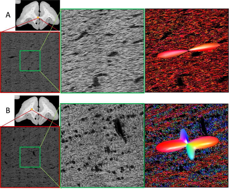
Qualitative confocal images. Representative confocal data (of a single slice) are shown for single (A) and crossing (B) fiber regions. Overview images highlight location of full 3D z-stacks (shown as a single, middle slice). A zoomed regions of interest in the middle of the z-stack (equivalent in size to an MRI voxel) are shown in the middle column. Results from structure tensor analysis are shown as color-coded images (with colors scheme as described in Figure 1), with the histologically-defined FOD overlaid as 3D glyphs (right).

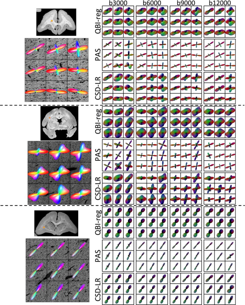
Histological 3D FODs derived from ST analysis are shown as glyphs overlaid on histology in Figure 3, displaying two regions containing crossing fibers (left and middle columns) and a single fiber region (right column). This highlights the ability of our histological procedures to resolve fibers crossing within a voxel where both fibers are in-plane (left), as well as the ability to detect bundles of fibers crossing in a plane orthogonal to confocal acquisition (middle). In addition, the results from all eight reconstruction methods are displayed below the corresponding histological FOD. All methods (except DTI) demonstrate some ability to resolve the crossing fibers in generally the same orientations as revealed by the histological FOD. However, differences between dMRI methods are apparent, particularly in the sharpness and number of peaks. For example, at the two extremes, QBIr results in a smoother function over a sphere than PAS, which results in distinct, sharp peaks. Similarly, in the single fiber region, all methods show qualitative agreement with histology in fiber orientation, with the only differences being overall lobe width (or dispersion), and sometimes small spurious peaks (most readily apparent in PAS and DOT).

Figure 3.

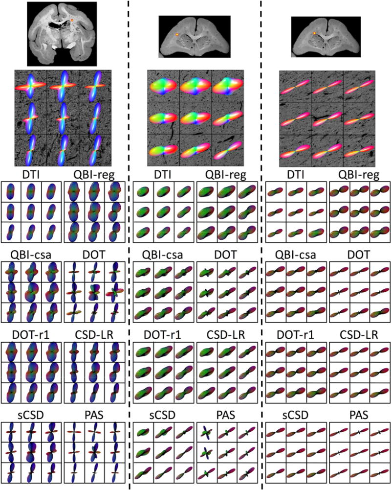
Effects of fiber geometry on reconstruction accuracy - qualitative results. Histological FODs are shown overlaid on confocal images for three z-stacks. Z-stack locations are shown as yellow boxes overlaid on 2D confocal montages (top). The voxels represent typical crossing fibers (left), fibers crossing both in-plane and through-plane (middle), and a typical single fiber regions (right). MRI data was analyzed at corresponding locations, and glyphs for all eight reconstruction methods are shown below each histological slice. Note that DTI results are displayed as the ADC profile.

Single Fiber and Crossing Fiber Regions

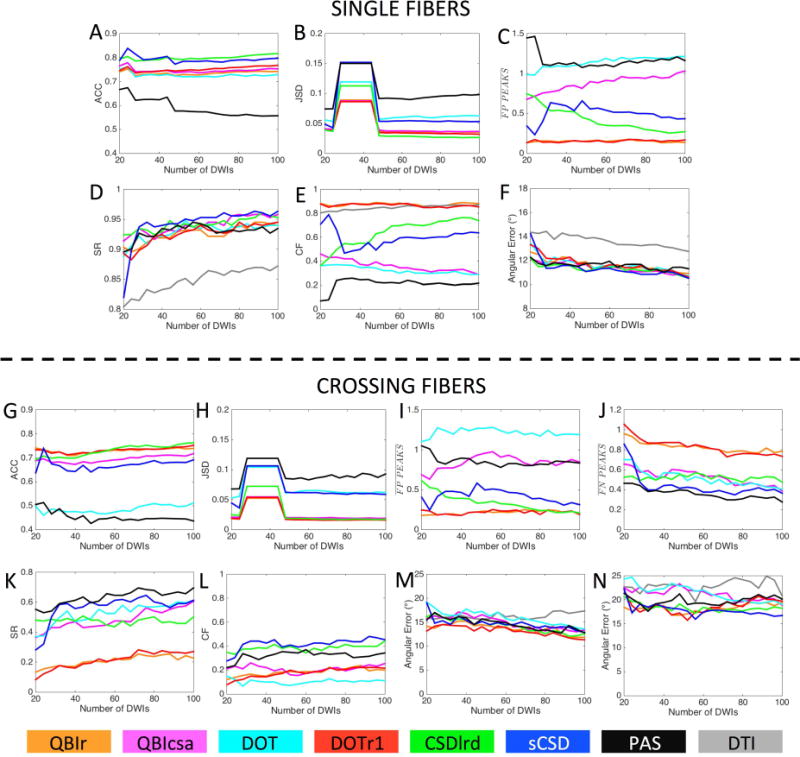
Quantitative comparisons between reconstruction methods for voxels containing single fiber geometries (N=383) and those containing crossing fiber geometries (N=181) are shown in Figure 4. All methods indicate good to moderate overall angular agreement with the histological FOD in single fiber regions, showing similar ACC results with median values between 0.73 and 0.80 for all methods. The one exception is PAS with a lower median ACC of 0.56 (Fig. 4A). The two methods with the highest ACC are those that estimate the FOD directly, sCSD and CSDlrd. Similarly, most methods show low JSD of <0.05, with the largest deviations occurring for PAS, DOT, and sCSD, respectively. The performance of each method with respect to estimation of the number of fiber populations in single fiber regions (Fig. 4C) shows that most methods consistently estimate a single peak. However, QBIcsa, DOT, and PAS consistently show the presence of FP peaks, with an average of ~2 peaks in these single fiber regions. The ability of all methods to successfully identify the single peak remains high (SR>93% for HARDI models) for all methods (including DTI) (Fig. 4D), however, the CF varies dramatically across models (Fig. 4E). For example, PAS, QBIcsa, and DOT have low CF, largely due to the prevalence of false positive peaks. Finally, the angular error in single fiber regions is remarkably consistent across all methods, with a median value of ~10° (Fig. 4F).

Figure 4.

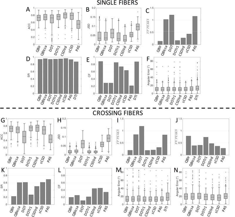
Effects of fiber geometry on reconstruction accuracy in single fiber (top) and crossing fiber (bottom) regions. Quality metrics describing overall agreement with the histological FOD (ACC: angular correlation coefficient, JSD: Jensen-Shannon Divergence), correct assessment of number of peaks (FP: false positive, FN: false negative, SR: success rate, CF: consistency fraction), and orientation accuracy (angular error), are shown for all HARDI methods, and DTI where appropriate.

The quantitative metrics show similar trends in crossing fiber regions (Fig. 4, G–N). The ACC is decreased slightly compared to that in single fiber regions (Fig. 4G) with a median ACC between 0.7 and 0.76 for all methods except DOT and PAS, which indicate a lower overall angular correlation with the ground truth FOD. Similarly, the JSD remains low for all methods, with the largest deviations occurring for PAS, DOT, and sCSD, respectively (Fig. 4H). In these regions, QBIcsa, DOT and PAS still contain a large number of FP peaks (Fig. 4I), while QBIr and DOTr1 show the largest prevalence of FN peaks (Fig. 4J), indicating the lowest ability to resolve crossing fibers. These two methods also show the lowest SR (Fig. 4K) with all other methods able to resolve the multiple fiber populations >50% of the time. However, all methods have low CF in crossing fiber regions (Fig. 4L), due to the frequency of FP and FN peaks. The median angular error of the primary peak (defined by histology) is consistently between 11–13°, a value slightly higher than that in single fiber regions. The exception to this is DTI (median value of 18°), which is unable to resolve multiple fiber populations, and the primary orientation is expected to lie somewhere between the two dominant peaks. The angular error of the non-dominant peaks is larger still, with a median value between 16° and 20° for all HARDI methods (we note that if a given reconstruction method did not contain multiple peaks, its lone peak is included only in one of the angular metrics, the one giving the lowest error).

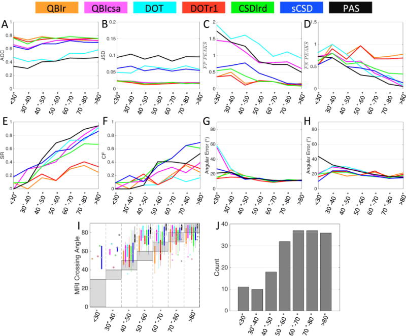
Crossing Angle

To assess under which geometrical conditions these methods succeed/fail in crossing fiber regions, we re-examine the quality metrics as a function of fiber crossing angle (Figure 5). First, voxels were grouped by crossing angle and placed into bins with a width of 10°, ranging from those with intra-fiber angle <30° to a maximum angle of 80–90°. Each bin had a sample size of 10 or greater (Fig 5J).

Figure 5.

Effects of crossing angle on reconstruction accuracy in crossing fiber regions. Quality metrics (A-H) are evaluated for all reconstruction methods as a function of histologically defined crossing angle, grouped into bins with widths of 10°. In addition, MRI-resolved crossing angle is compared to that from histology (I), and sample sizes for each angular bin (J) are shown. Reconstruction methods are designated by color.

Crossing angle has very little effect on ACC (Fig. 5A) and JSD (Fig. 5B) measures, although a slight increase in ACC with increasing angle is noticeable for PAS, QBIcsa, DOT, and sCSD. For all methods, the number of FP peaks is dramatically reduced as fibers cross at more orthogonal angles (Fig. 5C), with a similar reduction in FN peaks for QBIcsa, DOT, CSDlrd, sCSD, and PAS at larger angles (Fig. 5D). The reduction in both FP and FN peaks leads to a significant increase in SR (Fig. 5E) and CF (Fig. 5F) for all methods. In fact, QBIcsa, DOT, CSDlrd, sCSD, and PAS are able to successfully resolve nearly all peaks (SR near 1) at angle >80°. Besides angles <40°, the angular error for both primary (Fig. 5G) and secondary (Fig. 5H) fiber orientation is not dramatically affected by crossing angle. The increased angular error at small crossing angles is likely caused by reconstruction methods resolving multiple fiber populations, with only one accurately corresponding to one of the two histological peaks, and the other being a spurious peak and contributing to a larger error, or the dMRI finding only one peak with a primary orientation somewhere between the two true peaks.

Finally, Figure 5,I shows boxplots of the MRI-resolved angles (if the given reconstruction method was able to resolve multiple fiber populations) versus the histologically defined crossing angle. The shaded box highlights where the range of crossing angles should be if there was a perfect match in each histological angular bin. First, many methods do not show boxplots (or only have a single data point) in voxels with low crossing angles (in agreement with the low SR with these fiber geometries). Second, it is obvious that nearly all methods over-estimate the intra-voxel crossing angle. This effect is most noticeable in the 40–50° and 50–60° range. With very few exceptions, the MRI reconstruction methods consistently resolve fibers crossing at a more orthogonal angle than is suggested by the histological FOD.

Fiber Dispersion

We next examine the effect of fiber orientation dispersion on accuracy of MRI reconstruction methods. Histological analysis revealed a range of dispersion in the confocal z-stacks. Figure 6 provides a qualitative reference for the dispersion values investigated in this study, visualized as both 3D glyphs as well as surface distributions over a sphere. The ODI ranges from very highly aligned bundles with a low ODI (0.02–0.03, corresponding to a fiber spread of ~7–9°), to ODI more typical of WM voxels (0.08–0.13, a fiber spread of ~17–19°), to ODI > 0.40 (a fiber spread >37°).

Figure 6.

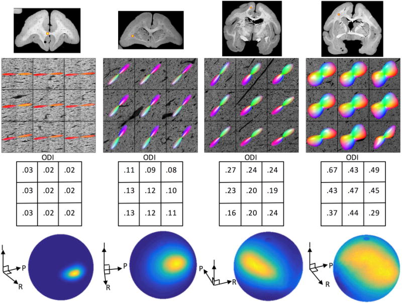
Histological dispersion in the brain WM. A range of fiber orientation dispersion is shown, ranging from low ODI (left) to high ODI (right). Dispersion is visualized with both 3D glyphs as well as orientation distributions on a sphere (for the center voxel of each stack). We note that ODI values between 0.08–0.13 are most typical of WM encountered in this study (in voxels containing single fiber populations).

We begin by examining the relationship between fiber dispersion derived from the 3D histological FOD (in single fiber regions only) and those derived from MRI reconstruction methods, as well as the relationship between dispersion and accuracy of fiber orientation estimates. (Figure 7). Plots of histological ODI versus orientation error indicate a low, but significant, positive correlation for all methods (Fig. 7A). Plotting the MRI-estimated ODI versus that from histology (Fig. 7B) shows moderate correlation for all methods, except for DOT. While correlation coefficients are similar, differences between methods are noticeable. For example, sCSD and PAS consistently result in low dispersion indices, while the QBI methods tend to overestimate ODI. Finally, for most methods, some form of an ODI lower bound is present, below which a resulting ODI is not possible due to either modeling assumptions, or the truncated spherical harmonic representation of the function.

Figure 7.

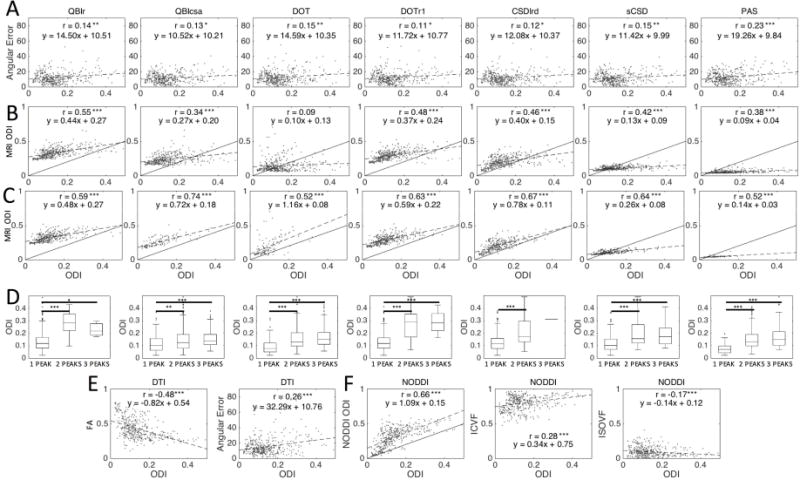
Effects of histological dispersion on MRI orientation and dispersion measures. MRI angular error (A) and MRI ODI estimates (B) are plotted against histological ODI in single fiber voxels. For all methods, large histological ODI consistently resulted in two or more distinct MRI peaks (D), and when FP voxels are removed, MRI-ODI correlations with histology-ODI are increased (C). DTI measures of FA and angular error (E), and NODDI measures of ODI, ICVF, and ISOVF (F) are plotted against histology-ODI. Significance levels are indicated by asterisks (*p<0.05; **p<0.01; ***p<0.001).

A potential source of discrepancy between MRI and histological measures of dispersion could be the presence of false positive peaks estimated with dMRI, causing a bias in ODI estimation. We find that many of the histological single fiber voxels with larger dispersion were separated into two or more distinct FP peaks using all reconstruction methods (Fig. 7D). In all cases, larger dispersion was significantly more likely to result in resolving 2 or more peaks. When voxels with FP peaks were removed from the analysis, all methods estimated dispersion indices with a much stronger correlation with histology (Fig. 7C), with correlation coefficients ranging from 0.52 for PAS to 0.74 for QBIcsa. Next, DTI FA shows a moderate, negative correlation with histological ODI, and the DTI angular error shows a small positive correlation (Fig. 7E). Finally, the NODDI multi-compartment model has a much stronger overall correlation with histological ODI (Fig. 7F) than the HARDI models (compare to Fig. 7B). We note that NODDI systematically overestimates the true ODI in our ex vivo experiments, although the line of best fit retains a slope near unity (m=1.09). However, there is also some low, but significant, correlation with the estimated intra-cellular volume fraction (ICVF) and isotropic volume fraction (ISOVF).

3.2 Effects of Number of DW Directions on Reconstruction Accuracy

Qualitative Results

We next examine the effects of the number of acquired DWIs (gradient directions) on reconstruction accuracy and quality metrics. Qualitative results are shown in Figure 8 for three selected HARDI methods. Here we focus on a region with fibers crossing at acute angles (top), a region containing fibers crossing at near-orthogonal angles (middle), and a single fiber region (bottom). For sharp crossing angles (top), while significant differences exist between methods, there is very little noticeable change between the 64 and 96 direction glyphs within methods. At 32 directions, peaks tend to “blend” into each other (see QBI-csa and DOTr1) or orientations are no longer consistent with histology (sCSD). Remarkably, at regions of orthogonal crossings (middle) almost no difference is observable across gradient directions, with all methods visually indicating the presence of crossing fibers. Similarly, in single fiber regions (bottom) no difference is observed as the number of DWIs varies.

Figure 8.

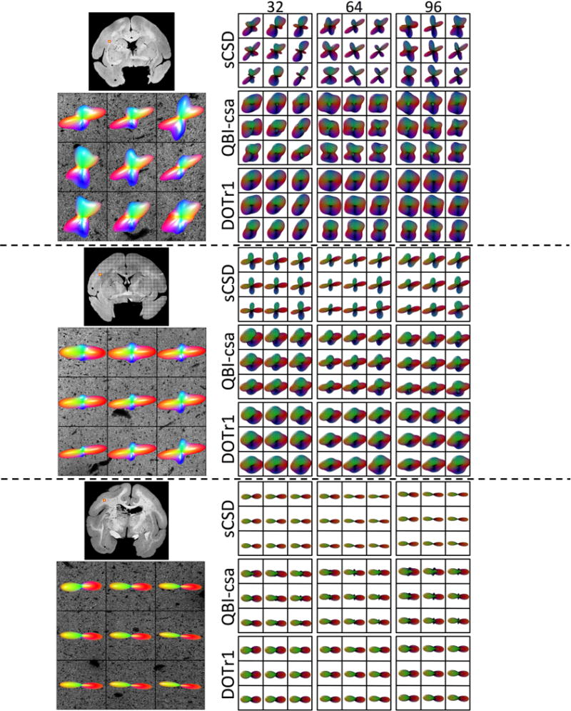
Effects of number of DW directions on reconstruction accuracy - qualitative results. Histological FODs are shown overlaid on confocal images for three z-stacks. The voxels represent fibers crossing at sharp angles (top), fibers crossing at near-orthogonal angles (middle), and a typical single fiber region (bottom). MRI-derived glyphs for three selected reconstruction methods are shown for each histological slice.

Single Fiber and Crossing Fiber Regions

Quantitative analysis of the effects of number of DW directions is shown in Figure 9. For these results, it is important to point out that the SH representation of all functions over a sphere use a maximum SH order of 4 for 20–24 directions, a maximum order of 6 for 28–44 directions, and a maximum order of 8 for 48 directions, or greater.

Figure 9.

Effects of number of DW directions on reconstruction accuracy in single fiber (A-F) and crossing fiber (G-N) regions. Quality metrics are evaluated for all modeling methods as a function of the number of DWIs (i.e. number of gradient directions) used in reconstruction. Reconstruction methods are designated by color.

For single fiber regions, all methods show a slight decrease in ACC (Fig. 9A) from 24 to 28 directions, and a slow, but consistent increase in ACC as directions increase (except for PAS). Also, there is little to no change in the rankings of the models across directions, for example sCSD and CSDlrd retain the highest ACC at all directions. Results for JSD (Fig. 9B) show very distinct changes when changing the SH order used to represent the functions. Specifically, the changes as the number of DW directions vary is much smaller than the changes in JSD when changing SH order, with noticeable increase in JSD at a 6^th order representation. The response to changing number of directions as it relates to FP peaks varies across methods (Fig. 9C). DOT and QBIcsa show an increasing prevalence of FP peaks as the number of DWIs increase, while PAS and CSDlrd show decreasing number of FP peaks, and QBIr and DOTr1 show very little change. The SR shows continuous improvement with increasing directions, with the greatest improvement apparent between 20 and 30 directions (Fig. 9D). The CF (Fig. 9E) shows trends inversely mirroring that of the FP peaks; QBIr and DOTr1 retain high, but consistent CF, PAS and CSDlrd show increasing CF with directions, with DOT and QBIcsa decreasing in CF. Finally, the angular error (Fig. 9F) continually decreases with increasing directions, with all HARDI methods showing very similar results, and DTI indicating the largest overall error.

Results in crossing fiber regions show similar trends. All methods (except for PAS) indicate a slight increase in ACC (Fig. 9G) with increasing directions, with the greatest increase occurring for CSDlrd (overtaking all other methods after 52 directions). Again, JSD is most sensitive to the SH order (Fig. 9H), rather than number of directions, with 6^th order showing the largest divergence from ground truth data. The number of FP peaks (Fig. 9I) again varies between methods, mirroring the trends seen in the single fiber analysis (see Fig. 9C). In all cases increasing image volumes regularizes the reconstruction, resulting in decreasing FN peaks (Fig. 9J), with the largest changes occurring between 20 and 30 directions, most notably for sCSD. Both the SR (Fig. 9K) and CF (Fig. 9L) for all methods show consistent increases as DW directions increase, continuing all the way to the full 100 directions. All methods show consistent behavior in these trends, with no obvious “optimal” number above which increases are diminishing. Finally, all methods (except DTI) show a slow, but continuous increase in orientation accuracy for both primary (Fig. 9M) and secondary (Fig. 9N) fiber orientations, with larger improvements apparent for the primary fiber orientations.

Number of DW directions and Crossing Angle

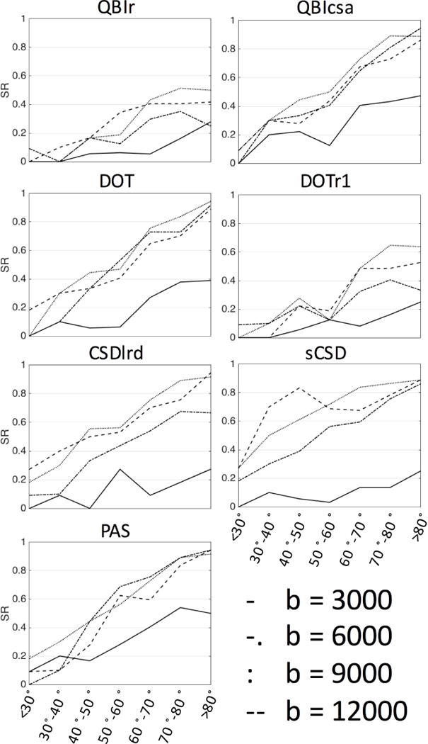
The SR for all methods is plotted as a function of histological crossing angle and number of DW directions in Figure 10 for all reconstruction methods. A few general trends are noticeable. Unsurprisingly, the SR increases as the intra-voxel angle increases (in agreement with Fig. 5E), and increases as the number of DW directions increases. Interestingly, for many methods, one can appreciate a sharp increase in SR at 70–80° and >80° range as the number of directions reaches 28 or greater. In addition, a similar increase in SR is apparent for the intermediate crossing angles (50–60° and 60–70° range) at directions ranging from as low as ~36 for PAS to approximately 60–64 directions for sCSD, QBIcsa, DOT, and CSDlrd. Finally, methods such as PAS, sCSD, QBIcsa, and DOT consistently show greater SR than QBIr and DOTr1, regardless of fiber geometry and acquisition parameters.

Figure 10.

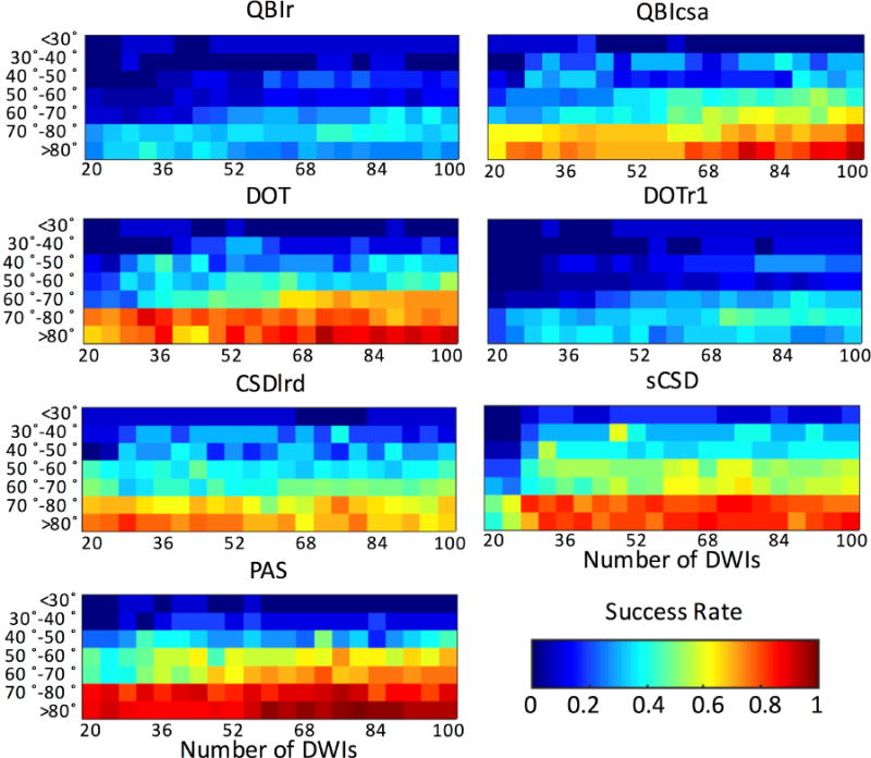
Effects of histological crossing angle and number of DWIs on SR of reconstruction methods.

3.3 Effects of b-value on Reconstruction Accuracy

Qualitative Results

Finally, we examine the effects of diffusion weighting (b-value) on the MRI reconstruction methods. Qualitative results are shown in Figure 11 for 3 select HARDI methods, in 3 different anatomical locations. Again, we have a region with near-orthogonal, clearly separated fibers (top), a region of sharp crossing fibers (middle), and a region with single fiber voxels (bottom). In these figures, it is apparent that the QBIr and CSDlrd methods are better able to resolve crossing fibers at higher b-values (>6,000 s/mm² in these regions), which also result in sharper FOD/ODF profiles. For PAS, the profiles do not appear to get “sharper”, but the orientations seem to differ across diffusion weightings. However, even at low b-values, all methods show a general agreement with the histologically defined FOD in crossing and single fiber regions. There are no readily apparent differences in the spherical profiles of the methods in the single fiber regions.

Figure 11.

Effects of b-value on reconstruction accuracy - qualitative results. Histological FODs are shown overlaid on confocal images for three z-stacks. The voxels represent fibers crossing at near-orthogonal angles (top), fibers crossing at acute angles (middle), and a typical single fiber region (bottom). MRI-derived glyphs for three selected reconstruction methods are shown for each histological slice.

Single Fiber and Crossing Fiber Regions

The effects of b-value on accuracy of MRI-reconstructions are shown in Figure 12 for single fiber (top) and crossing fiber (bottom) voxels. For single fiber regions, the b-value has varying effects on ACC (Fig. 12A), with methods like QBIr and DOTr1 showing clear improvement as b-value increases, while DOT and sCSD show improvement at lower b-values. For JSD (Fig. 12B), most methods show an increased divergence at higher b-values, with exceptions for QBIr and DOTr1. QBIr retains a low number of FP peaks at all diffusion weightings (Fig. 12C), PAS shows a decreasing FP rate once the b-value is increased above 3,000 s/mm², and all other methods show a clear increase in FP prevalence at higher b-values. The SR (Fig. 12D) remains high for all methods, with very little difference between methods, and little difference between b-values from 6,000–12,000 s/mm². However, the CF (Fig. 12E) is effected by the increased FP rate at high b-value, showing significant decreases for all HARDI methods. Finally, the angular error shows minor improvements at increasing b-values (Fig. 12F), for all methods.

Figure 12.

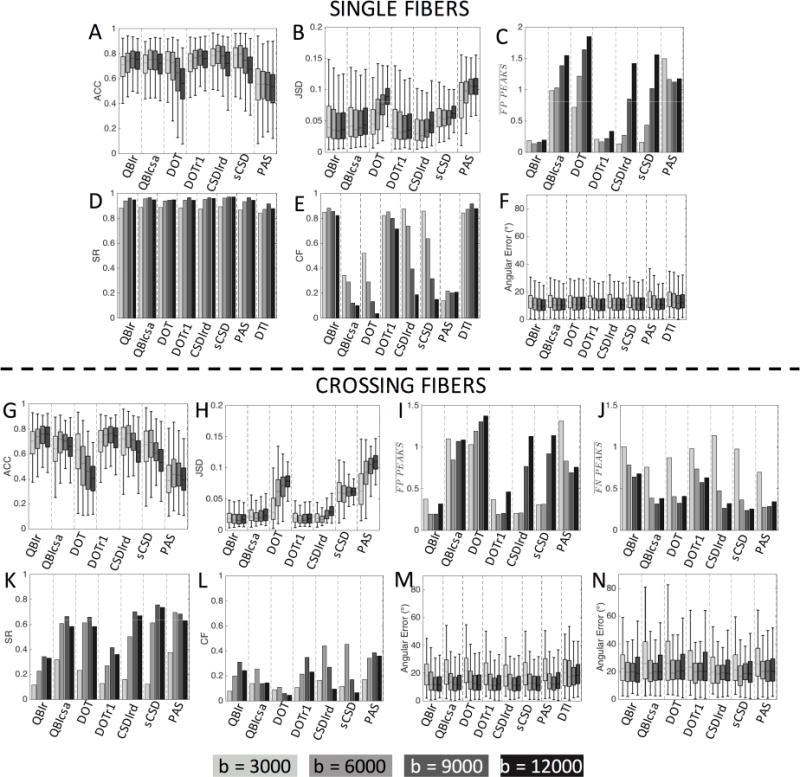
Effects of b-value on reconstruction accuracy in single fiber (A-F) and crossing fiber (G-N) regions. Quality metrics are evaluated for all modeling methods as a function of the diffusion-weighting used in reconstruction. b-values (in s/mm²) are indicated by gray-scale level.

The effects of b-value on MRI-reconstructions in crossing fiber regions show similar trends. The ACC (Fig. 12G) closely mirrors that in single fiber regions, although at a lower overall correlation. The JSD (Fig. 12H) indicates decreased performance at higher b-values for most methods, in particular DOT and PAS. Again, most methods show an increased number of FP peaks at larger diffusion weightings (Fig. 12I), with the largest increases observed for CSDlrd and sCSD. PAS shows the opposite trend, with the QBI methods showing a decreased FP rate at b-values of 6,000 and 9,000 s/mm². All methods show significant decreases in the number of FN peaks with b-values greater than 3,000 s/mm² (Fig. 12J). At a b-value of 3,000 s/mm² all methods consistently result in a single fiber population (a FN rate near 1). The decreased FN rate leads to increases in SR (Fig. 12K) for all methods at higher b-value, with the largest differences seen between 3,000 and 6,000 s/mm². Similarly, the CF (Fig. 12L) remains low at a b-value of 3,000 s/mm², peaking at either a b-value of 6,000 or 9,000 s/mm² for all methods. Finally, the angular error is largest in both the primary (Fig. 12M) and secondary (Fig. 12N) peaks for the b-value of 3,000, with little change seen when increasing diffusion weightings beyond 6,000 s/mm².

b-value and Crossing Angle

The SR of all-reconstruction methods at all b-values is plotted as a function of histological crossing angle in Figure 13. As before, and for all b-values, the resolving ability of all reconstruction methods increases as the crossing angle becomes larger. Also, for all methods, the data at b=3,000 s/mm² consistently has the lowest SR for all fiber configurations. At the low b-value, PAS tends to be the most successful at resolving fibers, at all crossing angles. For all methods, the SR generally increases at higher b-values, with smaller differences between b=6,000 and b=12,000 s/mm². At the lower crossing angles, sCSD tends to have the highest success (at b-values of 6,000 s/mm² or greater).

Figure 13.

Effects of histological crossing angle and b-value (in s/mm²) on success ratio (SR) of reconstruction methods.

4. Discussion

While there are a large number of dMRI methods for estimating neuronal fiber orientation distributions, the correspondence between dMRI measures and realistic biological fiber architectures remains unclear. Towards this end, this study investigated the relationship between the 3D histologically-defined distribution of neuronal fibers (the FOD) and the corresponding dMRI estimated orientation distributions, implementing a wide range of high angular resolution diffusion imaging techniques. Estimates of fiber orientation and anisotropy have previously been reported in biological tissue (Budde and Annese, 2013), and compared to DTI indices (Choe et al., 2012; Leergaard et al., 2010; Seehaus et al., 2015) and a high angular resolution QBI model (Leergaard et al., 2010); however, these methods have been limited to 2D histological measurements and small sample sizes. Recent work with confocal microscopy (Jespersen et al., 2012; Schilling et al., 2016), optical coherence tomography (Wang et al., 2015), and polarized light imaging (Axer et al., 2016; Mollink et al., 2017) extend the ability to extract the fiber orientation distributions to 3 dimensions. Still, no 3D histological validation of orientation and dispersion measures has been performed for any existing dMRI reconstruction techniques. Further, no histological validation study has presented a comparison of models, nor studied the effects of fiber geometry (crossing fibers, fiber dispersion) and acquisition parameters (number of DWIs, b-value, etc.) on their performance.

The most pertinent questions addressed in our study are whether the current generation of dMRI reconstruction methods allow us to adequately infer the underlying voxel-wise fiber orientations, and how algorithmic differences (including acquisition schemes, assumptions in modeling, descriptors used to characterize the intra-voxel structure, etc.) affect the fidelity of the resulting reconstruction. While we do not attempt a final ranking of the models (because the optimal technique is almost certainly going to depend on the intended goals and interests of the specific study) we are able to make some general observations, and report on the strengths and weaknesses of the tested dMRI algorithms.

All HARDI models are shown to describe the overall angular structure of the FOD, as evidenced by high ACC and low JSD in voxels containing both simple and complicated figure geometries (shown qualitatively in Figure 3, and quantified in Figure 4). Despite correlating well with the overall FOD shape, no method is consistently successful at extracting discrete measures of the number and orientations of FOD peaks. The major inaccuracies of all techniques tend to be in extracting or capturing local maxima of the FOD, resulting in either false positives and false negatives. Regardless of acquisition parameters, all methods show improved successes at resolving multiple fiber compartments in a voxel when fiber populations cross at near-orthogonal angles (Figures 5, 10, 13). This is consistent with the literature on both phantoms (Lin et al., 2003; Tournier et al., 2008) and simulations (Alexander, 2005; Daducci et al., 2014) and describes one of the major hurdles to resolving crossing fiber populations. In addition, the ability to resolve crossing fibers increases for all reconstruction methods at increased diffusion weightings (Figure 13), often at the expense of increased FP peaks and an overall lower overall angular agreement with the histological FOD (Figure 12). Thus, although techniques tend to capture the overall continuous shape of the FOD, care must be taken when evaluating diffusion results, particularly with respect to estimates of number of fibers or fiber orientation based on local maxima of the FOD or ODF alone.

A comparison across methods showed that no HARDI model outperformed others in every quality criteria or experimental condition. There was nearly always a tradeoff in measures of accuracy. For example, PAS regularly had the highest rate of success in resolving crossing fibers, at acute angles with low b-values and fewer gradient directions, however it is plagued with FP peaks in all conditions, and consistently had the lowest overall angular agreement with the FOD in both single and crossing fiber regions. On the other end of the spectrum, QBIr rarely resulted in identification of multiple maxima of the ODF, however, resulted in some of the highest ACC and lowest JSD values in all acquisition conditions. At first glance, the lack of consistency across models and wide range of accuracy in describing the FOD may be disheartening, the most commonly implemented (single-shell) HARDI methods for the last decade give varying results, and will almost certainly result in even more dramatic differences with subsequent fiber tracking. However, these results are unsurprising; the techniques all differ a great deal not only in modeling assumptions, but also what they aim to represent. One could envision a model based on the empirically derived FODs in this study, or some combination of techniques to obtain an optimal reconstruction. Another reassurance is that techniques show robustness to acquisition parameters including b-value (≥ 6,000 s/mm² for most methods in this ex vivo study) and number of DW directions, indicating that studies implementing the same reconstruction technique are likely to be comparable even with somewhat different acquisition parameters.

The robustness to the number of acquired DW directions is particularly surprising. Upon introduction of many techniques, a large number of directions are used. For example, 492 (Tuch et al., 2003), 252 (Tuch, 2004), and 80 directions (Tournier et al., 2008) for QBI methods, 60 (Tournier et al., 2004), 92 (Anderson, 2005), and 80 directions (Tournier et al., 2008) for spherical deconvolution methods, and 82 (Ozarslan et al., 2006) directions for DOT methods. For many methods, validation studies (often through simulation) show that with a moderate number of directions (>~50), methods show success at describing fiber geometries(Alexander, 2005; Alexander and Barker, 2005; Prckovska et al., 2013; Wilkins et al., 2015). Our results are generally in agreement with this observation, suggesting that many methods show an improvement at moderate numbers of directions (particularly in resolving intermediate crossing angles, Figure 10). However, the overall correlation with the histological FOD and other quality metrics (SR, false peaks) remain high for as few as 28 directions (Figure 9), a protocol common in many DTI schemes. Further, we find that some measures of quality (i.e. JSD and FP peaks) are largely influenced by the fit SH order used to represent that function on a sphere, an effect observed in previous reproducibility studies (Schilling et al., 2017c).

In addition to validating HARDI methods’ ability to capture orientation and number of fiber populations, we also validate the ability to capture another descriptor of fiber geometry, orientation dispersion. We tested a popular multi-compartment diffusion technique (NODDI) that estimates indices of neurites that may be more directly related to, and provide specific markers of, brain tissue microstructure. Measures of orientation dispersion may provide specificity for various pathologies (Billiet et al., 2014; By et al., 2017; Schneider et al., 2017; Wen et al., 2015), as well as provide fiber “tract-specific” indices that can again correlate to pathology, or increase fiber tracking specificity (Dell’Acqua et al., 2013; Raffelt et al., 2012; Riffert et al., 2014). Validation of dispersion measures has been performed for NODDI in the ex vivo spinal cord (Grussu et al., 2017) and on a 2-compartment dispersion model in the human corpus callosum (Mollink et al., 2017). In this study, we evaluate both signal models (which primarily aim to recover only the angular component of the diffusion profile) and the NODDI multi-compartment model (Figure 7). We find that the FOD and ODFs from signal models can provide more information that just number of peaks and peak directions. Specifically, the width of the FOD (or ODF) lobe is correlated with the histological fiber dispersion, for all reconstruction methods (significant correlations from r=0.34–0.55). High dispersion typically results in false positive peaks which can lead to errors in dispersion measures when fitting to Watson (or multi-Watson) distributions. When removing false positive peaks from analysis, the correlation is much stronger (r=0.52–0.74). Despite the high correlation, there is an overall limited range of dispersion identifiable with these techniques. For example, PAS and sCSD result in consistently low ODI (and sharp peaks), while QBIr and QBIcsa consistently result in larger ODI values. In addition, we find that increasing dispersion leads to greater uncertainty in estimating the primary fiber orientation in a voxel. For the NODDI model, which explicitly estimates a dispersion index, we find a much greater overall correlation (without the removal of FP peaks because NODDI estimates only a single fiber compartment). Overall, this demonstrates that the orientation dispersion estimates from dMRI correlate well with tissue architecture, using both HARDI and the multi-compartment NODDI model.

A recent study (Wedeen et al., 2012) proposed that the brain’s white matter structure is organized in a pattern of parallel sheets by analyzing crossing fiber pathways using dMRI tractography. It was found that incident pathways cross nearly orthogonally in a grid-like or sheet-like structure, with this pattern found throughout white matter and across species. This pattern has significant implications with regard to development, evolution, and structural connectivity. However, it has been argued (Catani et al., 2012) that this grid pattern is likely an artifact due to the inherently low angular resolution of the proposed dMRI technique (which estimated the diffusion ODF), causing a bias towards orthogonal angles, making the grid pattern a likely apparent geometric configuration. Our results indicate that all methods studied show a bias towards orthogonal crossings (Figure 5I), regardless of true histological crossing angle, and regardless of whether the FOD or ODF (or any other function) is estimated. This would seem to argue in favor of a technical limitation causing an artefactual grid. However, we note that (although we did not perform systematic random sampling) it was much easier to find near-orthogonal crossings than crossing angles less than 50° in the histological sections we studied (Figure 5J).

Future work should investigate the effects of reconstruction accuracy as spatial resolution varies. Because of the tradeoffs in spatial resolution, signal to noise ratio, and imaging time, optimizing the resolution for diffusion MRI (and subsequent analysis and/or tractography) is highly relevant to human in vivo imaging. Interestingly, recent work using MRI and high resolution histology has shown that the crossing fiber problem is not eliminated even with very high spatial resolution data (Schilling et al., 2017a). However, it is expected that the angular accuracy of diffusion MRI estimates will increase at high spatial resolution (Gangolli et al., 2017) due to reduced geometric complexity or decreased fiber dispersion (Gangolli et al., 2017; Schilling et al., 2017a).

While validation comparing dMRI and histology is the only validation method able to capture both the enormous complexity of the white matter in addition to the practical effects of image acquisition, it is not without limitations. Histology is technically complex due to tissue deterioration during preparation (shrinking, deformation, etc.). We have attempted to ameliorate the shrinkage with confocal image pre-processing, and a previous study describing the methodology (Schilling et al., 2016) shows an expected error of less than 5° when compared to manually traced fibers. In addition, to assess whether residual anisotropy or bias is introduced during confocal processing, we have evaluated the angular error as a function of the z-component of the histological FOD (Supplementary Figure 1) and found only very low correlations (maximum correlation of coefficient of |r| = 0.20). Only one reconstruction method (DTI) showed a statistically significant correlation (interestingly, a negative correlation as through-plane orientation increased). Together, this suggests that the angular error is largely independent of the histological FOD orientation. The multi-step registration procedure accounts for both deformation and tissue placement on the slide, and can result in localization errors on the order of the size of MRI voxels (Choe et al., 2011), 300 um in our study. Together, these may account for the slightly larger angular error than that seen in simulation studies (Alexander and Barker, 2005; Daducci et al., 2014; Jones, 2010; Landman et al., 2007), however, a median angular error of 10° is consistent with previous 2D histological validation studies on DTI (Choe et al., 2012; Leergaard et al., 2010). Thus, rather than a methodological limitation, this could indicate that the models used in simulation (often mixtures of Gaussians) are overly simplistic relative to the complicated true FOD that may not only contain disperse mixtures of fiber populations, but also varying microstructure affecting the motion of water, and anisotropic dispersion causing differences between the peak amplitude and something similar to an angular “center-of-mass” of the FOD. A further limitation is that confocal data, acquired in 50 micron tissue sections was compared to dMRI data acquired in 300 micron thick MRI sections. This comparison is based on the assumption that histological FODs change slowly in the slice direction, which is likely false in some fraction of voxels (and may account for some of the outliers in Figs 4 and 12, for example). While the present research focused on distinguishing “single” and “crossing” fibers, this may be an oversimplification of the true geometry. For example, in our confocal data, fibers are often seen bending throughout the field of view, and even within a voxel. Voxels can have both a dispersion and/or bending of fibers, yet result in a single local maximum of the FOD. Future work should utilize confocal data to quantify not only fiber curvature and bending, but also characterize how fibers cross and fan out (or in) within the voxel, and how these geometries relate to the diffusion signal. One final limitation of our study is extrapolation of the ex vivo tissue and imaging conditions to that of in vivo. However, previous studies indicate that anisotropy and the angular dependence of the signal is preserved (Dyrby et al., 2011; McNab et al., 2009; Schilling et al., 2017b), albeit at a lower diffusivity, thus care must be taken in interpreting the equivalent in vivo diffusion weightings for this study. Overall, there is no perfect validation method for dMRI, and we must rely on the accumulation of evidence from all approaches to validate and better understand the relationship between the dMRI signal and the tissue microstructure.

5. Conclusions

This work compared and evaluated fiber orientation distributions and orientation dispersion values derived from a number of diffusion MRI algorithms with those derived from histology. The algorithms included commonly implemented high angular resolution techniques for recovering intra-voxel fiber geometries, as well as a multi-compartment model. All reconstruction techniques are able to recover the overall angular structure of the FOD with some accuracy, with weaknesses in extracting discrete orientations and numbers of peaks. In addition, both HARDI methods and the microstructural model show high correlations with histologically defined orientation dispersion. These results can be used to identify the relative advantages of competing approaches, potential strategies for improving accuracy, and appropriate techniques to implement for answering specific research questions.

Supplementary Material

supplement

Supplementary Figure 1. Correlation between the absolute value of the z-component of the histological FOD (the through-plane component), and the angular error for all reconstruction methods. Statistical significance levels are indicated by asterisks (***p<0.001). Only one method, DTI, shows angular error dependency on the histological FOD orientation. The low correlation coefficients suggest that the confocal pre-processing and anisotropy corrections do not introduce a bias in orientation estimation.

Appendix A. Structure Tensor Analysis

To estimate the local orientation of fibers, structure tensor analysis (Bigun and Granlund, 1987) was applied to the entire 3D confocal image, f(x,y,z). The structure tensor is based on the gradient of the image intensity, f:

$$\nabla f_{\sigma }={(f_x,f_y,f_z)}^T$$ [A.1]

which is calculated with Gaussian derivative filters:

$$f_x=g_{x,\sigma }\ast f,f_y=g_{y,\sigma }\ast f,f_z=g_{z,\sigma }\ast f$$ [A.2]

where * denotes the convolution operation and g_x,σ, g_y,σ, and g_z,σ are the spatial derivatives in the x, y, and z-direction, respectively, of a 3D Gaussian with standard deviation σ:

$$g_{\sigma }(x,y,z)=\frac{1}{{(\sqrt{2\pi {\sigma }^2})}^3}{e}^{-\frac{(x^2+y^2+z^2)}{2{\sigma }^2}}$$ [A.3]

Next, an object known as the gradient square tensor, is calculated for each point in the image by taking the dyadic product of the gradient vector with itself:

$$\mathit{GST}(x,y,z)={\nabla f_{\sigma }\nabla f_{\sigma }}^T=\left(\begin{array}{ccc}{f}_x^2& f_x{f}_y& f_x{f}_z\\ f_x{f}_y& f_y^2& f_y{f}_z\\ f_x{f}_z& f_y{f}_z& f_z^2\end{array}\right)$$ [A.4]

Each tensor element is averaged over a local neighborhood to create the pixel-wise structure tensor. For spatial averaging, we choose a 3D Gaussian filter with standard deviation ρ:

$$S{T}_{\rho }(\nabla {\mathrm{f}}_{\sigma })=g_{\rho }\ast (\nabla f_{\sigma }\nabla f_{\sigma }^T)$$ [A.5]

This results in a 3-by-3 symmetric, semi-positive definite, rank-two tensor. Making the assumption that the direction of minimal intensity variation is parallel to the fiber at each pixel, fiber orientation is given by the direction of the eigenvector corresponding to the smallest eigenvalue.

The certainty in estimated fiber orientation can be described by the Westin-measure (Westin et al., 2002) which characterizes how planar the structure tensor is:

$$c_p=\frac{{\lambda }_2-{\lambda }_3}{{\lambda }_1}$$ [A.6]

where λ₁, λ₂, and λ₃ are the primary, secondary, and tertiary eigenvalues of the structure tensor. This value varies from 0 to 1 and will be large in areas where the first two eigenvalues are much larger than the third. This measurement is used to threshold the confocal image, so voxels with low certainties are not included in the final orientation distribution.

For the results presented in this paper, the spatial derivatives were calculated using a Gaussian with standard deviation σ = 1μm, and spatial averaging performed using a Gaussian with standard deviation ρ = 2.5μm.

Appendix B. Measures of similarity on the unit sphere (ACC and JSD)

A method for calculating the correlation of functions over a sphere given the SH expansions of both functions is given in (Anderson, 2005). Given two spherical functions and their spherical harmonic expansions:

$$\begin{array}{l}U(\theta ,\phi )={\displaystyle \sum _{l=0}^{\text{∞}}{\displaystyle \sum _{m=-l}^l{u}_{lm}{Y}_{lm}(\theta ,\phi )}}\\ V(\theta ,\phi )={\displaystyle \sum _{l=0}^{\text{∞}}{\displaystyle \sum _{m=-l}^l{v}_{lm}{Y}_{lm}(\theta ,\phi )}}\end{array}$$ [B.1]

The ACC of the functions is calculated as:

$$\mathit{ACC}=\frac{{\displaystyle {\sum }_{l=1}^{\text{∞}}{\displaystyle {\sum }_{m=-l}^l{u}_{lm}v{\ast }_{lm}}}}{{[{\displaystyle {\sum }_{l^{\prime }=1}^{\text{∞}}{\displaystyle {\sum }_{m^{\prime }=-l^{\prime }}^{l^{\prime }}|u_{l^{\prime }{m}^{\prime }}{|}^2}}]}^{1/2}{[{\displaystyle {\sum }_{l^{″}=1}^{\text{∞}}{\displaystyle {\sum }_{m^{″}=-l^{″}}^{l^{″}}|v_{l^{″}{m}^{″}}{|}^2}}]}^{1/2}}$$ [B.2]

The JSD was used to quantify the similarity between two FODs (or ODFs). Similar to (Cohen-Adad et al., 2011), we projected both FODs onto 724 values distributed equally over a sphere. The JSD is defined as

$$\mathit{JSD}(P,Q)=\frac{D_{KL}(P,M)+D_{KL}(Q,M)}{2}$$ [B.3]

with

$$M(i)=\frac{P(i)+Q(i)}{2}$$ [B.4]

and P(i) and Q(i) are the magnitudes of the histological and MRI FODs (or ODFs) along index i (i=1…724), and D_KL is the Kullback-Leibler divergence:

$$D_{KL}(P,Q)={\displaystyle \sum _{i}P(i)\text{log}\left(\frac{P(i)}{Q(i)}\right)}$$ [B.5]

References

- Aboitiz F, Scheibel AB, Fisher RS, Zaidel E. Fiber composition of the human corpus callosum. Brain Res. 1992;598:143–153. doi: 10.1016/0006-8993(92)90178-c. [DOI] [PubMed] [Google Scholar]
- Aganj I, Lenglet C, Sapiro G, Yacoub E, Ugurbil K, Harel N. Reconstruction of the orientation distribution function in single- and multiple-shell q-ball imaging within constant solid angle. Magn Reson Med. 2010;64:554–566. doi: 10.1002/mrm.22365. [DOI] [PMC free article] [PubMed] [Google Scholar]
- Alexander DC. Multiple-Fiber Reconstruction Algorithms for Diffusion MRI. Annals of the New York Academy of Sciences. 2005;1064:113–133. doi: 10.1196/annals.1340.018. [DOI] [PubMed] [Google Scholar]
- Alexander DC, Barker GJ. Optimal imaging parameters for fiber-orientation estimation in diffusion MRI. Neuroimage. 2005;27:357–367. doi: 10.1016/j.neuroimage.2005.04.008. [DOI] [PubMed] [Google Scholar]
- Alexander DC, Pierpaoli C, Basser PJ, Gee JC. Spatial transformations of diffusion tensor magnetic resonance images. Medical Imaging, IEEE Transactions on. 2001;20:1131–1139. doi: 10.1109/42.963816. [DOI] [PubMed] [Google Scholar]
- Anderson AW. Measurement of fiber orientation distributions using high angular resolution diffusion imaging. Magn Reson Med. 2005;54:1194–1206. doi: 10.1002/mrm.20667. [DOI] [PubMed] [Google Scholar]
- Anderson AW, Ding Z. Tenth Scientific Meeting of the International Society for Magnetic Resonance in Medicine. 2002. Sub-voxel measurement of fiber orientation using high angular resolution diffusion tensor imaging. [Google Scholar]
- Assaf Y, Basser PJ. Composite hindered and restricted model of diffusion (CHARMED) MR imaging of the human brain. Neuroimage. 2005;27:48–58. doi: 10.1016/j.neuroimage.2005.03.042. [DOI] [PubMed] [Google Scholar]
- Axer M, Strohmer S, Grassel D, Bucker O, Dohmen M, Reckfort J, Zilles K, Amunts K. Estimating Fiber Orientation Distribution Functions in 3D-Polarized Light Imaging. Front Neuroanat. 2016;10:40. doi: 10.3389/fnana.2016.00040. [DOI] [PMC free article] [PubMed] [Google Scholar]
- Basser PJ, Mattiello J, LeBihan D. MR diffusion tensor spectroscopy and imaging. Biophysical Journal. 1994;66:259–267. doi: 10.1016/S0006-3495(94)80775-1. [DOI] [PMC free article] [PubMed] [Google Scholar]
- Basser PJ, Pierpaoli C. Microstructural and physiological features of tissues elucidated by quantitative-diffusion-tensor MRI. J Magn Reson B. 1996;111:209–219. doi: 10.1006/jmrb.1996.0086. [DOI] [PubMed] [Google Scholar]
- Beaulieu C. The basis of anisotropic water diffusion in the nervous system - a technical review. NMR Biomed. 2002;15:435–455. doi: 10.1002/nbm.782. [DOI] [PubMed] [Google Scholar]
- Biggs DSC, Andrews M. Acceleration of iterative image restoration algorithms. Applied Optics. 1997;36:1766–1775. doi: 10.1364/ao.36.001766. [DOI] [PubMed] [Google Scholar]
- Bigun J, Granlund GH. Optimal Orientation Detection of Linear Symmetry. Proceedings of the IEEE First International Conference on Computer Vision. 1987:433–438. [Google Scholar]
- Billiet T, Madler B, D’Arco F, Peeters R, Deprez S, Plasschaert E, Leemans A, Zhang H, den Bergh BV, Vandenbulcke M, Legius E, Sunaert S, Emsell L. Characterizing the microstructural basis of “unidentified bright objects” in neurofibromatosis type 1: A combined in vivo multicomponent T2 relaxation and multi-shell diffusion MRI analysis. Neuroimage Clin. 2014;4:649–658. doi: 10.1016/j.nicl.2014.04.005. [DOI] [PMC free article] [PubMed] [Google Scholar]
- Budde MD, Annese J. Quantification of anisotropy and fiber orientation in human brain histological sections. Front Integr Neurosci. 2013;7:3. doi: 10.3389/fnint.2013.00003. [DOI] [PMC free article] [PubMed] [Google Scholar]
- By S, Xu J, Box BA, Bagnato FR, Smith SA. Application and evaluation of NODDI in the cervical spinal cord of multiple sclerosis patients. Neuroimage Clin. 2017;15:333–342. doi: 10.1016/j.nicl.2017.05.010. [DOI] [PMC free article] [PubMed] [Google Scholar]
- Canales-Rodriguez EJ, Lin CP, Iturria-Medina Y, Yeh CH, Cho KH, Melie-Garcia L. Diffusion orientation transform revisited. Neuroimage. 2010;49:1326–1339. doi: 10.1016/j.neuroimage.2009.09.067. [DOI] [PubMed] [Google Scholar]
- Canales-Rodriguez EJ, Melie-Garcia L, Iturria-Medina Y. Mathematical description of q-space in spherical coordinates: exact q-ball imaging. Magn Reson Med. 2009;61:1350–1367. doi: 10.1002/mrm.21917. [DOI] [PubMed] [Google Scholar]
- Caruyer E, Lenglet C, Sapiro G, Deriche R. Design of multishell sampling schemes with uniform coverage in diffusion MRI. Magn Reson Med. 2013;69:1534–1540. doi: 10.1002/mrm.24736. [DOI] [PMC free article] [PubMed] [Google Scholar]
- Catani M, Bodi I, Dell’Acqua F. Comment on “The geometric structure of the brain fiber pathways”. Science. 2012;337:1605. doi: 10.1126/science.1223425. [DOI] [PubMed] [Google Scholar]
- Chiang MC, Barysheva M, Lee AD, Madsen S, Klunder AD, Toga AW, McMahon KL, de Zubicaray GI, Meredith M, Wright MJ, Srivastava A, Balov N, Thompson PM. Brain fiber architecture, genetics, and intelligence: a high angular resolution diffusion imaging (HARDI) study. Med Image Comput Comput Assist Interv. 2008;11:1060–1067. doi: 10.1007/978-3-540-85988-8_126. [DOI] [PMC free article] [PubMed] [Google Scholar]
- Choe AS, Gao Y, Li X, Compton KB, Stepniewska I, Anderson AW. Accuracy of image registration between MRI and light microscopy in the ex vivo brain. Magn Reson Imaging. 2011;29:683–692. doi: 10.1016/j.mri.2011.02.022. [DOI] [PMC free article] [PubMed] [Google Scholar]
- Choe AS, Stepniewska I, Colvin DC, Ding Z, Anderson AW. Validation of diffusion tensor MRI in the central nervous system using light microscopy: quantitative comparison of fiber properties. NMR Biomed. 2012;25:900–908. doi: 10.1002/nbm.1810. [DOI] [PMC free article] [PubMed] [Google Scholar]
- Cohen-Adad J, Descoteaux M, Wald LL. Quality assessment of high angular resolution diffusion imaging data using bootstrap on Q-ball reconstruction. J Magn Reson Imaging. 2011;33:1194–1208. doi: 10.1002/jmri.22535. [DOI] [PMC free article] [PubMed] [Google Scholar]
- Cook PA, Symms M, Boulby PA, Alexander DC. Optimal acquisition orders of diffusion-weighted MRI measurements. J Magn Reson Imaging. 2007;25:1051–1058. doi: 10.1002/jmri.20905. [DOI] [PubMed] [Google Scholar]
- D’Arceuil HE, Westmoreland S, de Crespigny AJ. An approach to high resolution diffusion tensor imaging in fixed primate brain. Neuroimage. 2007;35:553–565. doi: 10.1016/j.neuroimage.2006.12.028. [DOI] [PubMed] [Google Scholar]
- Daducci A, Canales-Rodriguez EJ, Descoteaux M, Garyfallidis E, Gur Y, Lin YC, Mani M, Merlet S, Paquette M, Ramirez-Manzanares A, Reisert M, Reis Rodrigues P, Sepehrband F, Caruyer E, Choupan J, Deriche R, Jacob M, Menegaz G, Prckovska V, Rivera M, Wiaux Y, Thiran JP. Quantitative comparison of reconstruction methods for intra-voxel fiber recovery from diffusion MRI. IEEE Trans Med Imaging. 2014;33:384–399. doi: 10.1109/TMI.2013.2285500. [DOI] [PubMed] [Google Scholar]
- Dell’acqua F, Scifo P, Rizzo G, Catani M, Simmons A, Scotti G, Fazio F. A modified damped Richardson-Lucy algorithm to reduce isotropic background effects in spherical deconvolution. Neuroimage. 2010;49:1446–1458. doi: 10.1016/j.neuroimage.2009.09.033. [DOI] [PubMed] [Google Scholar]
- Dell’Acqua F, Simmons A, Williams SC, Catani M. Can spherical deconvolution provide more information than fiber orientations? Hindrance modulated orientational anisotropy, a true-tract specific index to characterize white matter diffusion. Hum Brain Mapp. 2013;34:2464–2483. doi: 10.1002/hbm.22080. [DOI] [PMC free article] [PubMed] [Google Scholar]
- Descoteaux M, Angelino E, Fitzgibbons S, Deriche R. Regularized, fast, and robust analytical Q-ball imaging. Magn Reson Med. 2007;58:497–510. doi: 10.1002/mrm.21277. [DOI] [PubMed] [Google Scholar]
- Dyrby TB, Baare WF, Alexander DC, Jelsing J, Garde E, Sogaard LV. An ex vivo imaging pipeline for producing high-quality and high-resolution diffusion-weighted imaging datasets. Hum Brain Mapp. 2011;32:544–563. doi: 10.1002/hbm.21043. [DOI] [PMC free article] [PubMed] [Google Scholar]
- Farrher E, Kaffanke J, Celik AA, Stöcker T, Grinberg F, Shah NJ. Novel multisection design of anisotropic diffusion phantoms. Magn Reson Imaging. 2012;30:518–526. doi: 10.1016/j.mri.2011.12.012. [DOI] [PubMed] [Google Scholar]
- Fieremans E, De Deene Y, Delputte S, Ozdemir MS, Achten E, Lemahieu I. The design of anisotropic diffusion phantoms for the validation of diffusion weighted magnetic resonance imaging. Phys Med Biol. 2008;53:5405–5419. doi: 10.1088/0031-9155/53/19/009. [DOI] [PubMed] [Google Scholar]
- Gangolli M, Holleran L, Hee Kim J, Stein TD, Alvarez V, McKee AC, Brody DL. Quantitative validation of a nonlinear histology-MRI coregistration method using generalized Q-sampling imaging in complex human cortical white matter. Neuroimage. 2017;153:152–167. doi: 10.1016/j.neuroimage.2017.03.059. [DOI] [PMC free article] [PubMed] [Google Scholar]
- Grussu F, Schneider T, Tur C, Yates RL, Tachrount M, Ianus A, Yiannakas MC, Newcombe J, Zhang H, Alexander DC, DeLuca GC, Gandini Wheeler-Kingshott CAM. Neurite dispersion: a new marker of multiple sclerosis spinal cord pathology? Ann Clin Transl Neurol. 2017;4:663–679. doi: 10.1002/acn3.445. [DOI] [PMC free article] [PubMed] [Google Scholar]
- Hong X, Arlinghaus LR, Anderson AW. Spatial normalization of the fiber orientation distribution based on high angular resolution diffusion imaging data. Magn Reson Med. 2009;61:1520–1527. doi: 10.1002/mrm.21916. [DOI] [PMC free article] [PubMed] [Google Scholar]
- Jansons KM, Alexander DC. Persistent Angular Structure: new insights from diffusion MRI data. Inf Process Med Imaging. 2003;18:672–683. doi: 10.1007/978-3-540-45087-0_56. [DOI] [PubMed] [Google Scholar]
- Jbabdi S, Sotiropoulos SN, Haber SN, Van Essen DC, Behrens TE. Measuring macroscopic brain connections in vivo. Nat Neurosci. 2015;18:1546–1555. doi: 10.1038/nn.4134. [DOI] [PubMed] [Google Scholar]
- Jespersen SN, Leigland LA, Cornea A, Kroenke CD. Determination of axonal and dendritic orientation distributions within the developing cerebral cortex by diffusion tensor imaging. IEEE Trans Med Imaging. 2012;31:16–32. doi: 10.1109/TMI.2011.2162099. [DOI] [PMC free article] [PubMed] [Google Scholar]
- Jeurissen B, Leemans A, Tournier JD, Jones DK, Sijbers J. Investigating the prevalence of complex fiber configurations in white matter tissue with diffusion magnetic resonance imaging. Hum Brain Mapp. 2013;34:2747–2766. doi: 10.1002/hbm.22099. [DOI] [PMC free article] [PubMed] [Google Scholar]
- Johansen-Berg H, Behrens TEJ. Diffusion MRI : from quantitative measurement to in-vivo neuroanatomy. 2nd. Elsevier/Academic Press; London, UK; Waltham, MA: 2014. [Google Scholar]
- Jones DK. Precision and accuracy in diffusion tensor magnetic resonance imaging. Top Magn Reson Imaging. 2010;21:87–99. doi: 10.1097/RMR.0b013e31821e56ac. [DOI] [PubMed] [Google Scholar]
- Jones DK, Cercignani M. Twenty-five pitfalls in the analysis of diffusion MRI data. NMR Biomed. 2010;23:803–820. doi: 10.1002/nbm.1543. [DOI] [PubMed] [Google Scholar]
- Landman BA, Farrell JA, Jones CK, Smith SA, Prince JL, Mori S. Effects of diffusion weighting schemes on the reproducibility of DTI-derived fractional anisotropy, mean diffusivity, and principal eigenvector measurements at 1.5T. Neuroimage. 2007;36:1123–1138. doi: 10.1016/j.neuroimage.2007.02.056. [DOI] [PMC free article] [PubMed] [Google Scholar]
- Leergaard TB, White NS, de Crespigny A, Bolstad I, D’Arceuil H, Bjaalie JG, Dale AM. Quantitative Histological Validation of Diffusion MRI Fiber Orientation Distributions in the Rat Brain. PLoS One. 2010;5:e8595. doi: 10.1371/journal.pone.0008595. [DOI] [PMC free article] [PubMed] [Google Scholar]
- Lin CP, Wedeen VJ, Chen JH, Yao C, Tseng WYI. Validation of diffusion spectrum magnetic resonance imaging with manganese-enhanced rat optic tracts and ex vivo phantoms. Neuroimage. 2003;19:482–495. doi: 10.1016/s1053-8119(03)00154-x. [DOI] [PubMed] [Google Scholar]
- McNab JA, Jbabdi S, Deoni SC, Douaud G, Behrens TE, Miller KL. High resolution diffusion-weighted imaging in fixed human brain using diffusion-weighted steady state free precession. Neuroimage. 2009;46:775–785. doi: 10.1016/j.neuroimage.2009.01.008. [DOI] [PubMed] [Google Scholar]
- Mollink J, Kleinnijenhuis M, Cappellen van Walsum AV, Sotiropoulos SN, Cottaar M, Mirfin C, Heinrich MP, Jenkinson M, Pallebage-Gamarallage M, Ansorge O, Jbabdi S, Miller KL. Evaluating fibre orientation dispersion in white matter: Comparison of diffusion MRI, histology and polarized light imaging. Neuroimage. 2017;157:561–574. doi: 10.1016/j.neuroimage.2017.06.001. [DOI] [PMC free article] [PubMed] [Google Scholar]
- Mori S, Crain BJ, Chacko VP, van Zijl PC. Three-dimensional tracking of axonal projections in the brain by magnetic resonance imaging. Ann Neurol. 1999;45:265–269. doi: 10.1002/1531-8249(199902)45:2<265::aid-ana21>3.0.co;2-3. [DOI] [PubMed] [Google Scholar]
- Mori S, van Zijl PCM. Fiber tracking: principles and strategies – a technical review. NMR Biomed. 2002;15:468–480. doi: 10.1002/nbm.781. [DOI] [PubMed] [Google Scholar]
- Ozarslan E, Shepherd TM, Vemuri BC, Blackband SJ, Mareci TH. Resolution of complex tissue microarchitecture using the diffusion orientation transform (DOT) Neuroimage. 2006;31:1086–1103. doi: 10.1016/j.neuroimage.2006.01.024. [DOI] [PubMed] [Google Scholar]
- Cook PA, Y B, Nedjati-Gilani S, Seunarine KK, Hall MG, Parker GJ, Alexander DC. Camino: Open-Source Diffusion-MRI Reconstruction and Processing; 14th Scientific Meeting of the International Society for Magnetic Resonance in Medicine; Seattle, WA, USA. May, 2006. p. 2759. [Google Scholar]
- Pawley JB, Masters RBR. Handbook of Biological Confocal Microscopy, Second Edition. Optical Engineering. 1996;35:2765–2766. [Google Scholar]
- Prckovska V, Achterberg HC, Bastiani M, Pullens P, Balmashnova E, Ter Haar Romeny BM, Vilanova A, Roebroeck A. Optimal short-time acquisition schemes in high angular resolution diffusion-weighted imaging. Int J Biomed Imaging. 2013;2013:658583. doi: 10.1155/2013/658583. [DOI] [PMC free article] [PubMed] [Google Scholar]
- Raffelt D, Tournier JD, Rose S, Ridgway GR, Henderson R, Crozier S, Salvado O, Connelly A. Apparent Fibre Density: a novel measure for the analysis of diffusion-weighted magnetic resonance images. Neuroimage. 2012;59:3976–3994. doi: 10.1016/j.neuroimage.2011.10.045. [DOI] [PubMed] [Google Scholar]
- Riffert TW, Schreiber J, Anwander A, Knosche TR. Beyond fractional anisotropy: extraction of bundle-specific structural metrics from crossing fiber models. Neuroimage. 2014;100:176–191. doi: 10.1016/j.neuroimage.2014.06.015. [DOI] [PubMed] [Google Scholar]
- Rohde GK, Aldroubi A, Dawant BM. The adaptive bases algorithm for intensity-based nonrigid image registration. IEEE Trans Med Imaging. 2003;22:1470–1479. doi: 10.1109/TMI.2003.819299. [DOI] [PubMed] [Google Scholar]
- Schilling K, Gao Y, Janve V, Stepniewska I, Landman BA, Anderson AW. Can increased spatial resolution solve the crossing fiber problem for diffusion MRI? NMR Biomed. 2017a doi: 10.1002/nbm.3787. [DOI] [PMC free article] [PubMed] [Google Scholar]
- Schilling K, Gao Y, Stepniewska I, Choe AS, Landman BA, Anderson AW. Reproducibility and variation of diffusion measures in the squirrel monkey brain, in vivo and ex vivo. Magn Reson Imaging. 2017b;35:29–38. doi: 10.1016/j.mri.2016.08.015. [DOI] [PMC free article] [PubMed] [Google Scholar]
- Schilling K, Janve V, Gao Y, Stepniewska I, Landman BA, Anderson AW. Comparison of 3D orientation distribution functions measured with confocal microscopy and diffusion MRI. Neuroimage. 2016;129:185–197. doi: 10.1016/j.neuroimage.2016.01.022. [DOI] [PMC free article] [PubMed] [Google Scholar]
- Schilling KG, Nath V, Blaber JA, Parvathaneni P, Anderson AW, Landman BA. Empirical consideration of the effects of acquisition parameters and analysis model on clinically feasible q-ball imaging. Magn Reson Imaging. 2017c;40:62–74. doi: 10.1016/j.mri.2017.04.007. [DOI] [PMC free article] [PubMed] [Google Scholar]
- Schneider T, Brownlee W, Zhang H, Ciccarelli O, Miller DH, Wheeler-Kingshott CG. Sensitivity of multi-shell NODDI to multiple sclerosis white matter changes: a pilot study. Funct Neurol. 2017;32:97–101. doi: 10.11138/FNeur/2017.32.2.097. [DOI] [PMC free article] [PubMed] [Google Scholar]
- Seehaus A, Roebroeck A, Bastiani M, Fonseca L, Bratzke H, Lori N, Vilanova A, Goebel R, Galuske R. Histological validation of high-resolution DTI in human post mortem tissue. Front Neuroanat. 2015;9:98. doi: 10.3389/fnana.2015.00098. [DOI] [PMC free article] [PubMed] [Google Scholar]
- Tournier JD, Calamante F, Connelly A. Robust determination of the fibre orientation distribution in diffusion MRI: non-negativity constrained super-resolved spherical deconvolution. Neuroimage. 2007;35:1459–1472. doi: 10.1016/j.neuroimage.2007.02.016. [DOI] [PubMed] [Google Scholar]
- Tournier JD, Calamante F, Connelly A. MRtrix: Diffusion tractography in crossing fiber regions. International journal of imaging systems and technology. 2012;22:53–66. [Google Scholar]
- Tournier JD, Calamante F, Connelly A. Determination of the appropriate b value and number of gradient directions for high-angular-resolution diffusion-weighted imaging. NMR Biomed. 2013;26:1775–1786. doi: 10.1002/nbm.3017. [DOI] [PubMed] [Google Scholar]
- Tournier JD, Calamante F, Gadian DG, Connelly A. Direct estimation of the fiber orientation density function from diffusion-weighted MRI data using spherical deconvolution. Neuroimage. 2004;23:1176–1185. doi: 10.1016/j.neuroimage.2004.07.037. [DOI] [PubMed] [Google Scholar]
- Tournier JD, Yeh CH, Calamante F, Cho KH, Connelly A, Lin CP. Resolving crossing fibres using constrained spherical deconvolution: validation using diffusion-weighted imaging phantom data. Neuroimage. 2008;42:617–625. doi: 10.1016/j.neuroimage.2008.05.002. [DOI] [PubMed] [Google Scholar]
- Tuch DS. Q-ball imaging. Magn Reson Med. 2004;52:1358–1372. doi: 10.1002/mrm.20279. [DOI] [PubMed] [Google Scholar]
- Tuch DS, Reese TG, Wiegell MR, Makris N, Belliveau JW, Wedeen VJ. High angular resolution diffusion imaging reveals intravoxel white matter fiber heterogeneity. Magn Reson Med. 2002;48:577–582. doi: 10.1002/mrm.10268. [DOI] [PubMed] [Google Scholar]
- Tuch DS, Reese TG, Wiegell MR, Wedeen VJ. Diffusion MRI of complex neural architecture. Neuron. 2003;40:885–895. doi: 10.1016/s0896-6273(03)00758-x. [DOI] [PubMed] [Google Scholar]
- Van Essen DC, Ugurbil K. The future of the human connectome. Neuroimage. 2012;62:1299–1310. doi: 10.1016/j.neuroimage.2012.01.032. [DOI] [PMC free article] [PubMed] [Google Scholar]
- Wang H, Lenglet C, Akkin T. Structure tensor analysis of serial optical coherence scanner images for mapping fiber orientations and tractography in the brain. J Biomed Opt. 2015;20:036003. doi: 10.1117/1.JBO.20.3.036003. [DOI] [PMC free article] [PubMed] [Google Scholar]
- Wedeen VJ, Hagmann P, Tseng WY, Reese TG, Weisskoff RM. Mapping complex tissue architecture with diffusion spectrum magnetic resonance imaging. Magn Reson Med. 2005;54:1377–1386. doi: 10.1002/mrm.20642. [DOI] [PubMed] [Google Scholar]
- Wedeen VJ, Rosene DL, Wang R, Dai G, Mortazavi F, Hagmann P, Kaas JH, Tseng WY. The geometric structure of the brain fiber pathways. Science. 2012;335:1628–1634. doi: 10.1126/science.1215280. [DOI] [PMC free article] [PubMed] [Google Scholar]
- Wehrl HF, Bezrukov I, Wiehr S, Lehnhoff M, Fuchs K, Mannheim JG, Quintanilla-Martinez L, Kohlhofer U, Kneilling M, Pichler BJ, Sauter AW. Assessment of murine brain tissue shrinkage caused by different histological fixatives using magnetic resonance and computed tomography imaging. Histol Histopathol. 2015;30:601–613. doi: 10.14670/HH-30.601. [DOI] [PubMed] [Google Scholar]
- Wen Q, Kelley DA, Banerjee S, Lupo JM, Chang SM, Xu D, Hess CP, Nelson SJ. Clinically feasible NODDI characterization of glioma using multiband EPI at 7 T. Neuroimage Clin. 2015;9:291–299. doi: 10.1016/j.nicl.2015.08.017. [DOI] [PMC free article] [PubMed] [Google Scholar]
- Westin CF, Maier SE, Mamata H, Nabavi A, Jolesz FA, Kikinis R. Processing and visualization for diffusion tensor MRI. Medical Image Analysis. 2002;6:93–108. doi: 10.1016/s1361-8415(02)00053-1. [DOI] [PubMed] [Google Scholar]
- Wilkins B, Lee N, Gajawelli N, Law M, Lepore N. Fiber estimation and tractography in diffusion MRI: development of simulated brain images and comparison of multi-fiber analysis methods at clinical b-values. Neuroimage. 2015;109:341–356. doi: 10.1016/j.neuroimage.2014.12.060. [DOI] [PMC free article] [PubMed] [Google Scholar]
- Williams JH, Mepham BL, Wright DH. Tissue preparation for immunocytochemistry. J Clin Pathol. 1997;50:422–428. doi: 10.1136/jcp.50.5.422. [DOI] [PMC free article] [PubMed] [Google Scholar]
- Yanasak N, Allison J. Use of capillaries in the construction of an MRI phantom for the assessment of diffusion tensor imaging: demonstration of performance. Magn Reson Imaging. 2006;24:1349–1361. doi: 10.1016/j.mri.2006.08.001. [DOI] [PubMed] [Google Scholar]
- Zhang H, Schneider T, Wheeler-Kingshott CA, Alexander DC. NODDI: practical in vivo neurite orientation dispersion and density imaging of the human brain. Neuroimage. 2012;61:1000–1016. doi: 10.1016/j.neuroimage.2012.03.072. [DOI] [PubMed] [Google Scholar]
Associated Data
This section collects any data citations, data availability statements, or supplementary materials included in this article.
Supplementary Materials