Network module identification—a widespread theoretical bias and best practices

Abstract

Biological processes often manifest themselves as coordinated changes across modules, i.e., sets of interacting genes. Commonly, the high dimensionality of genome-scale data prevents the visual identification of such modules, and straightforward computational search through a set of known pathways is a limited approach. Therefore, tools for the data-driven, computational, identification of modules in gene interaction networks have become popular components of visualization and visual analytics workflows. However, many such tools are known to result in modules that are large, and therefore hard to interpret biologically.

Here, we show that the empirically known tendency towards large modules can be attributed to a statistical bias present in many module identification tools, and discuss possible remedies from a mathematical perspective. In the current absence of a straightforward practical solution, we outline our view of best practices for the use of the existing tools.

1. Introduction

The organisation of cells is thought to be inherently modular [1, 2]. Modules can be identified from high-dimensional, genome-wide datasets. Typically, in a first step, gene-wise scores—often obtained from a statistical test— are calculated. These scores reflect the degree of involvement of each gene in a biological process. In a second step, one tries to identify gene modules from plausible sets of candidates, based on their scores.

Module candidates typically correspond to predefined gene sets, such as pathways [3], or connected subnetworks of a network of interacting genes [4]. Predefined gene sets are easier to analyse and interpret, but obviously limited by existing knowledge. Functional interaction networks represent information on pairs of genes known to interact—directly or indirectly—in the same biological context. Edges in such networks can represent hypothetical or verified physical associations between the corresponding molecules, such as protein-protein, protein-DNA, metabolic pathways, DNA-DNA interactions, or functional associations, such as epistasis, synthetic lethality, correlated expression, or correlated biochemical activities [5, 6, 7]. Given a network of interacting genes, modules are typically identified as ‘hot spots’, i.e., sub-networks with an aggregation of high gene-level scores.

Hot spots can be identified visually, using drawings of biological networks, in which high-scoring genes are highlighted. However, drawings of genome-scale biological networks often resemble ‘hairballs’ that lack a clear correspondence between regions in the drawing and subnetworks, making the visual identification of hot spots difficult.

In practice, one commonly identifies modules computationally, substituting human visual perception of strongly highlighted regions by computational search for high aggregate scores in connected subnetworks. Scores are commonly aggregated using a normalised score function that ensures an identical score distribution among subnetworks of different sizes, given a null model for gene-level scores. The gene-level null model is often specified with the gene-level scores, or it is implicit, e.g., when the gene-level scores are derived from P-values.

Many algorithms are based on the score defined by jActiveModules [8], including PANOGA [9], dmGWAS [10], EW-dmGWAS [11], PINBPA [12], GXNA [13], and PinnacleZ [14]. Others, such as BioNet [15, 16] and Sig-Mod [17] are based on a score adapted to integer linear programming. These methods are also widely applied in the current literature [18, 19, 20, 21, 22, 14, 23, 24, 25, 26], even though the above approaches have been reported to consistently result in subnetworks that are large, and therefore difficult to interpret biologically [13, 27, 28]. Some versions of the approach have dealt with this issue by introducing heuristic corrections designed to remove the tendency towards large subnetworks [13, 27, 17]. A recent evaluation of several algorithms revealed that the efficacy of these corrections remains limited [28]. Other methods avoid dealing with the issue by allowing users to limit the size of the returned module [10, 11, 12, 13, 14, 29], which is problematic, as prior information about suitable settings of this parameter is typically not available.

Here, we uncover the statistical basis of the above-mentioned empirical tendency of module identification tools to return large networks. Clear examples allow us to illustrate the origins of this size bias in the construction of the score function, and to propose a mathematical construction of a new and unbiased score. Even though we are not able to give an efficient algorithm for the practical computation of the new score, we uncover a possible connection to extreme value theory that might serve as the basis of future algorithmic developments, and discuss our view of the currently best practical approaches to the unbiased identification of network modules.

2. Materials and Methods

2.1. The subnetwork identification problem

Most of the above-mentioned module identification methods are motivated as the maximisation over a set of (connected) subnetworks of a graph. In its basic form, its three inputs can be described as follows.

1. A graph G, corresponding to the functional interaction network, in which the nodes V = (v₁,…, v_N) correspond to molecules. By A(G) we denote the sets A ⊆ V that induce connected subnetworks in G. By A_k(G) we denote only those sets of size |A| = k, which we will also call k-subnetworks.

2. A set of P-values (p₁, …, p_N) that correspond to the statistical significance of observations associated with the N molecules. (Whenever P-values are not directly available, they can easily be obtained from scores, e.g., by a rank-based transformation.)

3. A score function s(A) : A(G) →ℝ that assigns a score to each connected subnetwork.

A solution to the subnetwork identification problem corresponds to a subnetwork A that maximises the score s(A) over A(G).

2.2. jActiveModules score function

The jActiveModules method [8] was one of the first published subnetwork identification methods. Given an input graph G and P-values (p₁, …, p_N), a first aggregate score z(A) for a k-subnetwork A ∊ A_k(G) is defined using Stoufer's Z-score method [30]:

$$z(A)=\frac{1}{\sqrt{k}}\sum _{i\in A}{z}_i,$$

where z_i = ϕ⁻¹ (1 – p_i), and ϕ⁻¹ is the inverse normal cumulative distribution function (CDF). The jActiveModules score s(A) is then obtained as

$$s(A)=\frac{z(A)-{\mu }_k}{{\sigma }_k},$$

where μ_k and σ_k are sampling estimates of mean and standard deviation of scores z(A) over all k-node sets A ⊆ V. Ideker et al. [8] evaluated the resulting score against a distribution of empirically obtained scores under random permutations of (p₁, …,p_N), corresponding to a null hypothesis of a random assignment of input gene-level scores to the nodes of the network.

3. Theory

3.1. Subnetwork scores S_k, $S_k^{\ast }$

By S_k we denote a random variable that describes the occurrence of k-subnetwork scores, with CDF F(x) = P(s(A) ≤ x | A ∊ A_k(G)). Similarly, we denote by $S_k^{\ast }$ the maximal k-subnetwork scores with CDF F(x) = P(max_A∊Ak(G) s(A) ≤ x). Below, we will discuss the distributions of S_k and $S_k^{\ast }$ under the null hypothesis.

3.2. Score normalisation

Per construction of the jActiveModules score function, and under a sufficient amount of sampling to determine μ_k and σ_k, S_k follows a standard normal distribution: S_k ∼ ℕ(0,1)[8]. Whenever, as here, the distribution of S_k is independent of k, we will call the underlying score s normalised. As we will show below, the size bias of the jActiveModules score is rooted in the fact that jActiveModules searches for a highest-scoring subnetworks, but that maximisation is not taken into account by the normalised score it employs in its search.

4. A widespread theoretical bias in network module identification

In this section we show that, under a normalised score, small subnetworks can be significantly high-scoring in their size class, but still low-scoring when compared to scores that occur by chance in larger networks, thus explaining the above-mentioned size bias, i.e., the tendency of jActiveModules and related methods to return large subnetworks.

To empirically explore the properties of the jActiveModules score function, we generated a sample network with 50 nodes from STRING interaction network [5], which we denote by G₅₀, by first initialising a graph G_current with a randomly chosen node from the STRING network. Then we iteratively extended G_current with a randomly chosen neighbour, until |G_current| = 50.

4.1. For small values of k, the number |A_k(G)| of k-subnetworks increases strongly with k

By definition, the null distribution of a normalised score over all k-subnetworks is identical for all values of k. What normalisation does not take into account is the fact that the number |A_k(G)| of k-subnetworks depends on k.

We now explore this effect for different graphs G. In a fully connected graph G, each k-subset A ⊆ V forms a k-subnetwork. Here, $\left|{\mathrm{A}}_k(G)\right|=\left(\begin{array}{c}N\\ k\end{array}\right)$, which strongly increases with increasing small k.

Figure 1 shows that, also for our sample network G = G₅₀, |A_k(G)| strongly increases with k for small k.

Figure 1. Numbers |A_k(G)| of small subnetworks in G₅₀ (a network of 50 nodes) as a function of their size k.

Finally, the STRING [5] network G with 250 000 highest-scoring edges has |A₃(G)| = 20 676 496 3-subnetworks, and |A₄(G)| = 201 895 916 4-subnetworks. The number of 5-subnetworks was higher yet; we were not able to determine |A₅(G)| in a reasonable amount of time by straightforward enumeration.

4.2. Maximum scores increase strongly with k under the null hypothesis

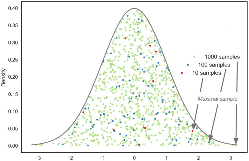
We now explore the behaviour of the maximum k-subnetwork score $S_k^{\ast }$ under the null hypothesis, with increasing k, for small values of k. As |A_k(G)| tends to increase strongly with small k (Section 4.1), and the distribution of jActiveModules scores S_k is independent of k (cf. Section 3.2), one may expect $S_k^{\ast }$ to strongly increase with k. Figure 2 illustrates this effect in the case of independent identically distributed (i.i.d.) samples.

Figure 2. Sample maxima from independent identically distributed samples are likely to increase with sample size.

Subnetwork scores S_k are not independent, as subnetworks in A_k(G) are overlapping. To explore whether the same effect as in the independent case can still be observed, we computed scores $S_k^{\ast }$ in our sample network G = G₅₀ for 100 000 random instantiations of (p₁, …, p₅₀). Figure 3 shows the resulting empirical distributions of $S_k^{\ast }$, for some small values of k, with a clear increase of $S_k^{\ast }$ with increasing k.

Figure 3. Empirical distributions of jActiveModules maximum subnetwork scores $S_k^{\ast }$ for small values of k under the null hypothesis.

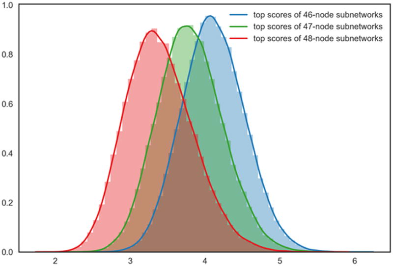
We note in passing that, for large values of k, the number |A_k(G)| of connected subnetworks must, at some point, decrease (note that |A_N(G)| = 1 for any connected graph G). Accordingly, one may expect decreasing maximum scores $S_k^{\ast }$ when k approaches N. Our empirical evaluation, shown in Figure A.1, is consistent with this idea: On our sample graph G₅₀, jActive-Modules scores $S_k^{\ast }$ decrease for k = 46, 47, 48.

4.3. Maximum scores may follow an extreme value distribution under the null hypothesis

Maxima of i.i.d. scores have been proven to follow an extreme value distribution [31] (Appendix B.1). However, due to the overlap between subnetworks, subnetwork scores S_k are not independent. Nevertheless, most pairs of small subnetworks of a larger network do not overlap, and their dependency structure is therefore local.

Extreme value distributions are used in other cases when dependency structure is local. They have been been proved to accurately approximate certain sequences of random variables whose high scores (block maxima) have a local dependency structure [31]. In sequence alignment, high-scoring alignments tend to overlap locally, and Karlin and Altschul [32] demonstrated that the null distribution of local similarity scores can be approximated by an extreme value distribution. Here, a weighting parameter K explicitly accounts for the non-independence of the positions of high-scoring matches. K is specific to the search database, and its estimation is computationally intensive.

Figure 4.3 shows that generalised extreme value distributions also fit empirically observed distributions $S_k^{\ast }$ quite well in the sample network G₅₀ (fit parameters given in Table 1; probability plots in Appendix C). The fit can be observed to be good for smaller values of k, and to deteriorate with increasing k, concomitant with the loss of locality in the subnetwork dependency structure.

Table 1. Parameters for the fits F(x; μ_k,σ_k, ξ_k) in Figure 4.3.

k	μk	σk	ξk
1	2.1	0.33	0.08
2	2.3	0.36	0.12
3	2.6	0.40	0.16
4	2.9	0.41	0.18
5	3.2	0.42	0.20

4.4. The jActiveModules score and other normalised scores are biased towards larger subnetworks

Our empirical study of maximal subnetwork scores suggests that maximum scores $S_k^{\ast }$ strongly increase under the null hypothesis when k is small (cf. Figure 3). This implies that certain non-significant subnetworks of larger size are systematically scored higher than other, smaller, subnetworks that have a significantly high score relative to their size. Figure 5 illustrates this effect: a score that is unlikely to be observed by chance in a 3-subnetwork is much more likely to be observed by chance in a 5-subnetwork. Even though we were not able to explicitly calculate $S_k^{\ast }$ for k > 5, we deem it likely that, larger k-subnetworks (with, say, k > 7) with even better scores are almost certain to exist in random data. As many methods do not provide an assessment of the statistical significance of the reported subnetworks, these methods not only prefer spurious larger subnetworks over—potentially biologically relevant—smaller ones, but also fail to provide their users with an indication that the reported networks are indistinguishable from chance observations.

Figure 5.

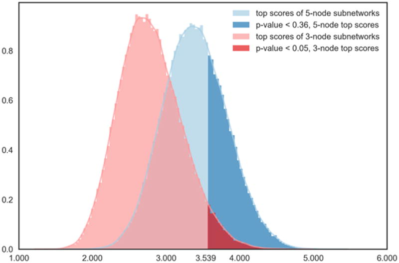
Scenario illustrating the bias of normalised scores towards larger subnetworks. Distributions shown are jActiveModules null distributions $S_3^{\ast }$ and $S_5^{\ast }$ for the sample network G50. Under the null hypothesis, a normalised score of 3.538 is unlikely to occur by chance for a 3-subnetwork A₃ $(P(S_3^{\ast }\ge \mathrm{3.538})\approx \mathrm{0.05})$, but the same score is much more likely to occur by chance for a 5-subnetwork A₅ $(P(S_5^{\ast }\ge \mathrm{3.538})\approx \mathrm{0.36})$. The unbiased score function s˜ takes this into account by scoring A₃ much higher than A₅: s˜(A₃) ≈ 1 – 0.05 = 0.95, but s˜(A₅) ≈ 1 – 0.36 = 0.64.

5. Unbiased module detection—theory and practice

5.1. An unbiased score function s˜

It is straightforward to mathematically remove the size bias of any (normalised or unnormalised) score s(A) by calibrating it relative to its size-specific null distribution (which requires taking into account the maximisation over subnetworks). For a k-subnetwork A, we define the score

$$\stackrel{\sim }{s}(A)={\stackrel{\sim }{s}}_k(A)=1-P(S_k^{\ast }\ge s(A)).$$

The negative sign of the P-value ensures the expected directionality of the score, i.e., that subnetworks with high aggregate gene-level scores receive a high score s˜. The resulting maximum scores ${\stackrel{\sim }{S}}_k^{\ast }$ are approximately uniformly distributed on [0,1], i.e., $P({\stackrel{\sim }{S}}_k^{\ast }\le x)\approx x$. Note that this correspondence is only approximate, as ${\stackrel{\sim }{S}}_k^{\ast }$ is a discrete distribution.

5.2. Computing the unbiased score s˜ by sampling is computationally hard, but it may be possible to approximate S˜ by an extreme value distribution

Even though the unbiased score s˜ can be easily defined, it is not straight-forward to compute it efficiently. In principle, s˜(A) could be approximated by sampling from $S_k^{\ast }$, but each sample requires the computation of a maximum of s(A) over all subnetworks A in a network — a problem that has been shown to be NP-hard even in a simplified form [8]. Approaches to solve this problem nonetheless exist [15, 17], but under the reported running times in the range of minutes to hours for a single sample from $S_k^{\ast }$, current approaches still remain impractical for any but the smallest networks.

The locality of the dependency structure among small subnetworks and our empirical results from Section 4.3 suggest that $S_k^{\ast }$ can possibly be approximated by an extreme value distribution. However, it is not obvious how the parameters of this distribution can be estimated practically without recourse to sampling, which, as discussed above, is impractical.

5.3. Current best practices for the unbiased identification of network modules

In the absence of practical solutions to compute the unbiased subnetwork score S˜, what are the current practical options for the unbiased scoring and detection of network modules?

One possibility is to use one of the approaches that find highest-scoring subnetworks of a fixed, or limited, subnetwork size k [16, 10, 11, 12, 13, 14, 29], and to evaluate these subnetworks on the basis of their biological interpretation. Since only small networks tend to be biologically interpretable, only small k would have to be tested. As the statistical significance of a subnetwork can be expected to be relatively stable upon removal or addition of a few neighbours, not all values of k would need to be tested. While this approach has obvious shortcomings (multiple statistical tests, often unclear biological interpretation), each computation by itself would only compare subnetworks of same size, and thus avoid size bias.

There are other, non-statistical (e.g., algorithmic/physical) principles for identifying aggregates of signals in networks [33, 34]. The lack of clear mathematical relationships between inputs and outputs, or lacking information about statistical significance may make it difficult to assess the properties of these approaches, and their applicability to any given biological scenario. The recently developed LEAN approach preserves mathematical clarity and statistical tools, and obtains computational tractability through a restriction to a simplified subnetwork model [35], whose significance for biological applications remains to be confirmed.

6. Conclusions

The identification of network modules of highest aggregate scores is an important approach to analyse biological datasets. In small and sparse networks, modules can be identified visually as regions of high gene-level scores, when visualised on top of network drawings, but this approach breaks down for large networks resulting from typical high-dimensional, genome-wide datasets. An array of methods and software addresses this problem computationally, but many of them are plagued by an empirically recognised strong tendency towards large subnetworks that ad hoc adjustments have not been able to remedy.

Here, we present a first direct analysis of the origins of this phenomenon, and uncover a strong statistical size bias in the underlying score function. By mathematical normalisation against size-specific null distributions, we derive a new, unbiased, score function. Straightforward computation of this score is computationally infeasible, and we outline our view of currently best other practical options on the basis of existing tools. Finally, we hope that our observation, demonstrating that the unbiased score function may be approximated using extreme value distributions, will motivate further practical developments towards the unbiased identification of modules in networks.

Highlights.

• The identification of network modules in genome-scale datasets is a long-standing problem.

• Current approaches tend to return large subnetworks that are hard to interpret.

• We identify a size bias in the score function underlying many of these approaches.

• We derive practical recommendations to minimize size bias using existing tools.

• Our new, unbiased, score function can be approximated using extreme value distributions.

Appendix A. For large values of k, maximal subnetwork scores decrease

Figure A.1. Distributions of maximum subnetwork scores $S_k^{\ast }$ for large values of k under the null hypothesis.

Appendix B. Approximate normality of subnetworks scores S_k

Figure B.1.

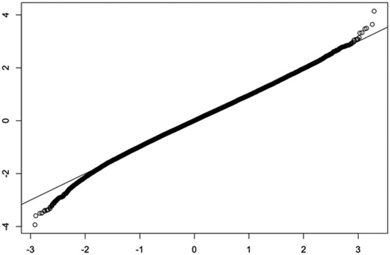
Quantile-quantile plot between standard normal distribution and jActiveModules scores S₅ for the sample graph G₅₀ under the null hypothesis. Other scores S_k have similar quantile-quantile plots (not shown).

Appendix C. Quality of extreme value distribution fits for maximal subnetwork scores $S_k^{\ast }$

Figure C.1. Probability plot for the extreme value model fit to maximal scores of subnetworks of size 1, $S_1^{\ast }$, in G₅₀.

Figure C.2. Probability plot for the extreme value model fit to $S_2^{\ast }$.

Figure C.3. Probability plot for the extreme value model fit to $S_3^{\ast }$.

Figure C.4. Probability plot for the extreme value model fit to $S_4^{\ast }$.

Figure C.5. Probability plot for the extreme value model fit to $S_5^{\ast }$.

Appendix D. Implementation: Code used to generate data for Figures in the main text

All plots have been generated using Python. jActiveModules Java code that has been modified to run independently from Cytoscape environment, and augmented with options used to generate Figures in the article, can be found in the github repository:

https://github.com/schwikowskilab/jActiveModulesHeadless/tree/paper

To compile, go into the main folder and execute mvn clean package.

To run, execute java -jar -Xss4m -Xmx14848M target/jActiveModulesHeadless-1.0.jar -help.

To generate the data used in the paper, use option -t with the available parameters.

Figure 1: Use −t 3. The option will calculate numbers of subnetworks starting from size 1 to number of nodes in the network. Here is an example:

java -jar -Xss4m -Xmx14848M target/jActiveModulesHeadless-1.0.jar -t 3 -nf testNetworkSmall 50nodes 136edges.sif -df testdata 50nodes.txt

Figure 2: Use −t 2. The number of samples from which you take the maximum is defined in the file src/main/resources/jActiveModules.props with the option AP.samplingIterationSize. The size of subnetworks is defined in the same file by AP.subnetworkSize. If you change any values in this file, you need to recompile the code to take modifications into account. The output is written to the output directory (by default jActiveModulesResults folder in your home directory) into file scoreTestInd.txt.

Figure 3: Use −t 1. The size of subnetworks is defined in

src/main/resources/jActiveModules.props by AP.subnetworkSize.

The output is written to the output directory (by default jActiveModulesResults folder in your home directory) into file scoreTest.txt.

Figure 4: Extreme value distributions have been fitted using stats.genextreme.fit() function of the stats package from the Python scipy environment (http://www.scipy.org/).

Figure 4. Fits of generalised extreme value distributions F(x; μ_k,σ_k,ξ_k) to empirical distributions of $S_k^{\ast }$.

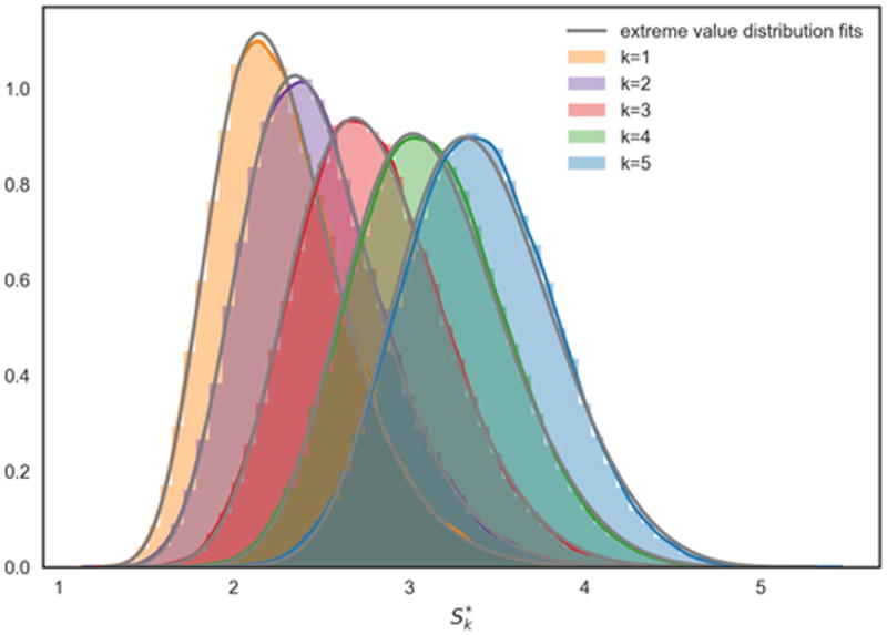
Figure 5: Distributions are an extract of the ones represented on Figure 3 (distributions for k=3 and k=5). Darker zones have been computed from this same data.

References

- 1.Alon U. Biological networks: the tinkerer as an engineer. Science (New York, N Y) 2003;301(5641):1866–7. doi: 10.1126/science.1089072. URL http://www.ncbi.nlm.nih.gov/pubmed/14512615. [DOI] [PubMed] [Google Scholar]
- 2.Hartwell LH, Hopfield JJ, Leibler S, Murray AW. From molecular to modular cell biology. Nature. 1999;402(6761 Suppl):C47–C52. doi: 10.1038/35011540. arXiv:0521865719 9780521865715. [DOI] [PubMed] [Google Scholar]
- 3.Khatri P, Sirota M, Butte AJ. Ten years of pathway analysis: Current approaches and outstanding challenges. PLoS Computational Biology. 8(2) doi: 10.1371/journal.pcbi.1002375. [DOI] [PMC free article] [PubMed] [Google Scholar]
- 4.Mitra K, Carvunis AR, Ramesh SK, Ideker T. Integrative approaches for finding modular structure in biological networks. Nature Reviews Genetics. 2013;14(10):719–732. doi: 10.1038/nrg3552. URL http://www.nature.com/doifinder/10.1038/nrg3552. [DOI] [PMC free article] [PubMed] [Google Scholar]
- 5.Szklarczyk D, Franceschini A, Wyder S, Forslund K, Heller D, Huerta-Cepas J, Simonovic M, Roth A, Santos A, Tsafou KP, Kuhn M, Bork P, Jensen LJ, von Mering C. STRING v10: protein-protein interaction networks, integrated over the tree of life. Nucleic acids research. 2014 Oct;43:447–452. doi: 10.1093/nar/gku1003. 2014. URL http://www.ncbi.nlm.nih.gov/pubmed/25352553. [DOI] [PMC free article] [PubMed] [Google Scholar]
- 6.Keshava Prasad TS, Goel R, Kandasamy K, Keerthikumar S, Kumar S, Mathivanan S, Telikicherla D, Raju R, Shafreen B, Venugopal A, Balakrishnan L, Marimuthu A, Banerjee S, Somanathan DS, Sebastian A, Rani S, Ray S, Harrys Kishore CJ, Kanth S, Ahmed M, Kashyap MK, Mohmood R, Ramachandra YI, Krishna V, Rahiman BA, Mohan S, Ranganathan P, Ramabadran S, Chaerkady R, Pandey A. Human Protein Reference Database -2009 update. Nucleic Acids Research. 2009;37(SUPPL. 1):767–772. doi: 10.1093/nar/gkn892. [DOI] [PMC free article] [PubMed] [Google Scholar]
- 7.Lee I, Blom UM, Wang PI, Shim JE, Marcotte EM. Prioritizing candidate disease genes by network-based boosting of genome-wide association data. Genome research. 2011;21(7):1109–21. doi: 10.1101/gr.118992.110. URL http://www.pubmedcentral.nih.gov/articlerender.fcgi?artid=3129253&tool=pmccentrez&rendertype=abstract. [DOI] [PMC free article] [PubMed] [Google Scholar]
- 8.Ideker T, Ozier O, Schwikowski B, Andrew F. Discovering regulatory and signalling circuits in molecular interaction networks. Bioinformatics. 2002;18(Suppl):233–240. doi: 10.1093/bioinformatics/18.suppl_1.s233. [DOI] [PubMed] [Google Scholar]
- 9.Bakir-Gungor B, Sezerman OU. A new methodology to associate SNPs with human diseases according to their pathway related context. PloS one. 2011;6(10):e26277. doi: 10.1371/journal.pone.0026277. URL http://www.pubmedcentral.nih.gov/articlerender.fcgi?artid=3201947&tool=pmcentrez&rendertype=abstract. [DOI] [PMC free article] [PubMed] [Google Scholar]
- 10.Jia P, Zheng S, Long J, Zheng W, Zhao Z. dmGWAS: dense module searching for genome-wide association studies in protein-protein interaction networks. Bioinformatics. 2011;27(1):95–102. doi: 10.1093/bioinformatics/btq615. URL http://www.pubmedcentral.nih.gov/articlerender.fcgi?artid=3008643&tool=pmcentrez&rendertype=abstract. [DOI] [PMC free article] [PubMed] [Google Scholar]
- 11.Wang Q, Yu H, Zhao Z, Jia P. EW dmGWAS: edge-weighted dense module search for genome-wide association studies and gene expression profiles. Bioinformatics. 2015 Mar;31:2591–2594. doi: 10.1093/bioinformatics/btv150. URL http://bioinformatics.oxfordjournals.org/cgi/doi/10.1093/bioinformatics/btv150. [DOI] [PMC free article] [PubMed] [Google Scholar]
- 12.Wang L, Matsushita T, Madireddy L, Mousavi P, Baranzini SE. PINBPA: Cytoscape app for network analysis of GWAS data. Bioinformatics. 2015;31(2):262–264. doi: 10.1093/bioinformatics/btu644. [DOI] [PubMed] [Google Scholar]
- 13.Nacu S, Critchley-Thorne R, Lee P, Holmes S. Gene expression network analysis and applications to immunology. Bioinformatics (Oxford, England) 2007;23(7):850–8. doi: 10.1093/bioinformatics/btm019. URL http://www.ncbi.nlm.nih.gov/pubmed/17267429. [DOI] [PubMed] [Google Scholar]
- 14.Chuang HY, Lee E, Liu YT, Lee D, Ideker T. Network-based classification of breast cancer metastasis. Molecular systems biology. 2007;3(140):140. doi: 10.1038/msb4100180. URL http://www.pubmedcentral.nih.gov/articlerender.fcgi?artid=2063581&tool=pmcentrez&rendertype=abstract. [DOI] [PMC free article] [PubMed] [Google Scholar]
- 15.Dittrich MT, Klau GW, Rosenwald A, Dandekar T, Müller T. Identifying functional modules in protein-protein interaction networks: an integrated exact approach. Bioinformatics (Oxford, England) 2008;24(13):i223–31. doi: 10.1093/bioinformatics/btn161. URL http://www.pubmedcentral.nih.gov/articlerender.fcgi?artid=2718639&tool=pmcentrez&rendertype=abstract. [DOI] [PMC free article] [PubMed] [Google Scholar]
- 16.Backes C, Rurainski A, Klau GW, Müller O, Stöckel D, Gerasch A, Küntzer J, Maisel D, Ludwig N, Hein M, Keller A, Burtscher H, Kaufmann M, Meese E, Lenhof HP. An integer linear programming approach for finding deregulated subgraphs in regulatory networks. Nucleic acids research. 2012;40(6):e43. doi: 10.1093/nar/gkr1227. URL http://www.pubmedcentral.nih.gov/articlerender.fcgi?artid=3315310&tool=pmcentrez&rendertype=abstract. [DOI] [PMC free article] [PubMed] [Google Scholar]
- 17.Liu Y, Brossard M, Roqueiro D, Margaritte-Jeannin P, Sarnowski C, Bouzigon E, Demenais F. SigMod: an exact and efficient method to identify a strongly interconnected disease-associated module in a gene network. Bioinformatics (January) 2017:btx004. doi: 10.1093/bioinformatics/btx004. URL http://bioinformatics.oxfordjournals.org/lookup/doi/10.1093/bioinformatics/btx004. [DOI] [PubMed]
- 18.Sharma A, Gulbahce N, Pevzner SJ, Menche J, Ladenvall C, Folkersen L, Eriksson P, Orho-Melander M, Barabási AL. Network-based analysis of genome wide association data provides novel candidate genes for lipid and lipoprotein traits. 2013 doi: 10.1074/mcp.M112.024851. URL http://www.ncbi.nlm.nih.gov/pubmed/23882023. [DOI] [PMC free article] [PubMed]
- 19.Olex AL, Turkett WH, Fetrow JS, Loeser RF. Integration of gene expression data with network-based analysis to identify signaling and metabolic pathways regulated during the development of osteoarthritis. Gene. 2014;542(1):38–45. doi: 10.1016/j.gene.2014.03.022. URL http://dx.doi.org/10.1016/j.gene.2014.03.022. [DOI] [PMC free article] [PubMed] [Google Scholar]
- 20.Smith CL, Dickinson P, Forster T, Craigon M, Ross A, Khondoker MR, France R, Ivens A, Lynn DJ, Orme J, Jackson A, Lacaze P, Flanagan KL, Stenson BJ, Ghazal P. Identification of a human neonatal immune-metabolic network associated with bacterial infection. Nature communications. 2014;5:4649. doi: 10.1038/ncomms5649. URL http://www.nature.com/ncomms/2014/140814/ncomms5649/full/ncomms5649.html%5. [DOI] [PMC free article] [PubMed] [Google Scholar]
- 21.Pérez-Palma E, Andrade V, Caracci MO, Bustos BI, Villaman C, Medina MA, Ávila ME, Ugarte GD, De Ferrari GV. Early Transcriptional Changes Induced by Wnt/ β -Catenin Signaling in Hippocampal Neurons. Neural Plasticity. 2016;2016:1–13. doi: 10.1155/2016/4672841. URL https://www.hindawi.com/journals/np/2016/4672841/ [DOI] [PMC free article] [PubMed] [Google Scholar]
- 22.Jin G, Zhou X, Wang H, Zhao H, Cui K, Zhang XS, Chen L, Hazen SL, Li K, Wong STC. The knowledge-integrated network biomarkers discovery for major adverse cardiac events. Journal of Proteome Research. 2008;7(9):4013–4021. doi: 10.1021/pr8002886. [DOI] [PMC free article] [PubMed] [Google Scholar]
- 23.Dao P, Wang K, Collins C, Ester M, Lapuk A, Sahinalp SC. Optimally discriminative subnetwork markers predict response to chemotherapy. Bioinformatics. 2011;27(13):205–213. doi: 10.1093/bioinformatics/btr245. [DOI] [PMC free article] [PubMed] [Google Scholar]
- 24.Liu M, Liberzon A, Sek WK, Lai WR, Park PJ, Kohane IS, Kasif S. Network-based analysis of affected biological processes in type 2 diabetes models. PLoS Genetics. 2007;3(6):0958–0972. doi: 10.1371/journal.pgen.0030096. [DOI] [PMC free article] [PubMed] [Google Scholar]
- 25.Qiu YQ, Zhang S, Zhang XS, Chen L. Detecting disease associated modules and prioritizing active genes based on high throughput data. BMC bioinformatics. 2010;11:26. doi: 10.1186/1471-2105-11-26. URL http://www.pubmedcentral.nih.gov/articlerender.fcgi?artid=2825224&tool=pmcentrez&rendertype=abstract. [DOI] [PMC free article] [PubMed] [Google Scholar]
- 26.Hormozdiari F, Penn O, Borenstein E, Eichler EE. The discovery of integrated gene networks for autism and related disorders. 2015 doi: 10.1101/gr.178855.114. [DOI] [PMC free article] [PubMed] [Google Scholar]
- 27.Rajagopalan D, Agarwal P. Inferring pathways from gene lists using a literature-derived network of biological relationships. Bioinformatics (Oxford, England) 2005;21(6):788–93. doi: 10.1093/bioinformatics/bti069. URL http://www.ncbi.nlm.nih.gov/pubmed/15509611. [DOI] [PubMed] [Google Scholar]
- 28.Batra R, Alcaraz N, Gitzhofer K, Pauling J, Ditzel HJ, Hellmuth M, Baumbach J, List M. On the performance of de novo pathway enrichment. npj Systems Biology and Applications. 2017;3(1):6. doi: 10.1038/s41540-017-0007-2. URL http://www.nature.com/articles/s41540-017-0007-2. [DOI] [PMC free article] [PubMed] [Google Scholar]
- 29.Beisser D, Klau GW, Dandekar T, Müller T, Dittrich MT. BioNet: an R-Package for the functional analysis of biological networks. Bioinformatics (Oxford, England) 2010;26(8):1129–30. doi: 10.1093/bioinformatics/btq089. URL http://www.ncbi.nlm.nih.gov/pubmed/20189939. [DOI] [PubMed] [Google Scholar]
- 30.Stouffer SA, Suchman EA, DeVinney LC, Star SA, Williams RM. The American soldier: Adjustment during Army life. (Studies in social psychology in World War II, Vol. I) Princeton University Press. 1949;28(1):87–90. URL http://dx.doi.org/10.2307/2572105. [Google Scholar]
- 31.Coles S. An Introduction to Statistical Modeling of Extreme Values. Springer Series in Statistics. 2001 [Google Scholar]
- 32.Karlin S, Altschul SF. Methods for assessing the statistical significance of molecular sequence features by using general scoring schemes. Proceedings of the National Academy of Sciences of the United States of America. 1990 Mar;87:2264–2268. doi: 10.1073/pnas.87.6.2264. [DOI] [PMC free article] [PubMed] [Google Scholar]
- 33.West J, Beck S, Wang X, Teschendorff AE. An integrative network algorithm identifies age-associated differential methylation interactome hotspots targeting stem-cell differentiation pathways. Scientific reports. 2013;3:1630. doi: 10.1038/srep01630. URL http://www.nature.com/articles/srep01630%5Cnhttp://www.pubmedcentral.nih.gov/articlerender.fcgi?artid=3620664&tool=pmcentrez&rendertype=abs. [DOI] [PMC free article] [PubMed] [Google Scholar]
- 34.Alcaraz N, Pauling J, Batra R, Barbosa E, Junge A, Christensen AGL, Azevedo V, Ditzel HJ, Baumbach J. KeyPathwayMiner 4.0: condition-specific pathway analysis by combining multiple omics studies and networks with Cytoscape. BMC systems biology. 2014;8(1):99. doi: 10.1186/s12918-014-0099-x. URL http://bmcsystbiol.biomedcentral.com/articles/10.1186/s12918-014-0099-x. [DOI] [PMC free article] [PubMed] [Google Scholar]
- 35.Gwinner F, Boulday G, Vandiedonck C, Arnould M, Cardoso C, Nikolayeva I, Guitart-Pla O, Denis CV, Christophe OD, Beghain J, Tournier-Lasserve E, Schwikowski B. Network-based analysis of omics data: The LEAN method. Bioinformatics (Oxford, England) 2016 Dec;33(5):701–709. doi: 10.1093/bioinformatics/btw676. 2016. URL http://www.ncbi.nlm.nih.gov/pubmed/27797778. [DOI] [PMC free article] [PubMed] [Google Scholar]