Clustal Omega for making accurate alignments of many protein sequences

Abstract

Clustal Omega is a widely used package for carrying out multiple sequence alignment. Here, we describe some recent additions to the package and benchmark some alternative ways of making alignments. These benchmarks are based on protein structure comparisons or predictions and include a recently described method based on secondary structure prediction. In general, Clustal Omega is fast enough to make very large alignments and the accuracy of protein alignments is high when compared to alternative packages. The package is freely available as executables or source code from www.clustal.org or can be run on‐line from a variety of sites, especially the EBI www.ebi.ac.uk.

Introduction

Clustal Omega1 is a package for making multiple sequence alignments (MSAs). It was developed almost a decade ago in response to greatly increasing numbers of available sequences and the need to make big alignments quickly and accurately. The most widely used packages for making MSAs over the past 30 years have been Clustal W2 and Clustal X3 but well over a hundred MSA packages have been released in that time. They have roughly fallen into two main groups: those that are fast and able to make very large alignments or those that are more accurate and restricted to smaller numbers of sequences. MUSCLE4 and MAFFT5 are widely used examples of the former while T‐Coffee6 and MAFFT L‐INS‐i7 are examples of the latter. Clustal W and Clustal X are widely used because of their widespread availability for personal computers and on servers and because of the robustness and portability of the code as well as the very flexible and intuitive user interface. Our original motivation, when designing Clustal Omega, was to make a package that could make very large alignments but without sacrificing accuracy.

The first Clustal package featured a fast and simple method for making “guide trees.”8 These are clusterings of the sequences that are used to decide the order of alignment during the later progressive alignment phase. Clustal is an example of a group of related methods that date back to the first fully automated MSA method from the 1970s.9 The general idea is to start with alignments of just two sequences, usually the closest ones in the dataset. The alignment is then built up by aligning alignments with each other or sequences to alignments, according to the topology of the guide tree. The complexity of the guide tree construction is usually O(N²) for N sequences because all N sequences have to be compared to each other. Earlier versions of Clustal used fast word based alignments for these comparisons which made it memory efficient and fast enough to work on PCs and Macintosh computers. However, as the number of sequences grows above a few thousand, the O(N²) complexity becomes very time consuming and makes very big alignments difficult to make. We developed an O(NlogN) method called mBed,10 that allows guide trees of hundreds of thousands of sequences to be made by restricting the calculation of sequence alignment scores to NLog(N). This mBed method is what is used in Clustal Omega to give capacity and scalability for very large datasets.

The second main development in Clustal Omega was to use an alignment engine for aligning profile hidden Markov models (HMMs) to each other instead of the conventional dynamic programing and profile alignment. We used HHalign11 which had been shown to have very high accuracy for profile HMM alignment. This gives greatly increased accuracy to Clustal Omega when compared to earlier Clustal programs, as measured on structure based alignment benchmarks. Only a small amount of original code from the earlier Clustal programs was used for the new program: the fast word‐based pairwise alignment routines. The rest of the code was coded new from scratch or taken from publically available libraries.

This gave a brand new program that was able to align many thousands of sequences without losing accuracy. It was released in 2011 and is freely available for download of all source code under an Open Source license. Users can also download executables for most operating systems (www.clustal.org) or use the program on‐line at many sites, especially the EMBL European Bioinformatics Institute (www.ebi.ac.uk). In this article, we wish to describe some features of Clustal Omega that have been added since the original release and to show some benchmark results of various program options using a recently described protein benchmark based on accuracy of secondary structure prediction.12

Benchmarking Clustal Omega

We will benchmark the performance of Clustal Omega, its various command‐line options and some other widely used programs using different data sets. The most well established benchmark for multiple sequence alignment is BAliBASE.13 Here, we will use BAliBASE version 3.0.14 It is comprised of 218 reference alignments, grouped into six categories: (BB11/12) equidistant sequences of similar length, (BB2) families containing orphan sequences, (BB3) equidistant divergent families, (BB4) N/C‐terminal extensions, and (BB5) alignments with insertions. The number of sequences of the reference alignments varies from four to 142, with a median of 21 sequences. Reference alignments range in length from 88 positions to 8481 and in average pairwise identity from 10.80% to 54.08%. We will measure the time and memory required to construct the test alignments and the quality of the alignments in terms of the sum‐of‐pairs (SP) score and the total column (TC) score. The SP score measures the fraction of aligned residue pairs that agree in the reference alignment and the test alignment. The TC score measures the fractions of columns that are perfectly aligned. As already one misplaced residue can nullify the contribution of an entire column, this score is much more severe than the SP score.

Another widely used MSA benchmark is Prefab. Prefab is a collection of 1682 reference sequence pairs, whose alignment is known, to which between 0 and 48 (median 48, mean 45.2) nonreference sequences are added. Prefab is therefore larger in terms of the number of families than BAliBASE 3.0 with its 218 families. With 50 versus 21, Prefab's median number of sequences per alignment is larger than in BAliBASE 3.0, but BAliBASE 3.0 has a larger maximum number of sequences per alignment (142 versus 50). The longest sequence in Prefab is 1132 residues long, while in BAliBASE 3.0 this value is 7923. A qualitative difference between Prefab and BAliBASE is that in BAliBASE every sequence is a reference sequence and contributes to assessing the alignment quality. In Prefab, however, there are only two reference sequences which determine the alignment quality. Alignment of the nonreference sequences does not impact on the score given to the alignment. This is particularly true if in the guide‐tree the two reference sequences are aligned early on. No sequence that is aligned to the reference sequences after this can modify the relative positioning of the residues in the reference sequences.

The largest alignment in BAliBASE, in terms of sequence number, has 142 sequences. BAliBASE can therefore not stress test MSA software regarding memory or time usage for large datasets. A benchmark that is comprised of families with up to almost 100,000 sequences is HomFam.10 In HomFam, a few sequences with a known alignment are blended with a large number of homologous sequences with an unknown alignment. The reference alignments are derived from Homstrad15 and the bulk of sequences come from Pfam.16 The MSA is performed of all the sequences in a HomFam family, however, the quality can only be assessed for the few Homstrad sequences. Using HomFam, one can certainly exercise MSA software for large numbers of sequences but scoring the alignment may be unreliable. This may occur, if the Homstrad and Pfam sequences separate in the guide‐tree due to length mismatches or homology. That way the effective size of the alignment that can be probed may be reduced to not much more than the number of reference sequences. We will use HomFam to exhibit memory and CPU consumption only. We will not use the entire HomFam data set of 95 families but only some example families. To show the scalability of the execution times we will use a very short protein domain (Homstrad: zf‐CCHH; PF00096 Zinc finger C2H2 type; length range 23 to 34 residues), a medium length domain (Homstrad: rvp; PF00077 Retroviral aspartyl protease; length range: 94 to 124) and a long protein domain (Homstrad: RuBisCO_large; PF00016 Ribulose bisphosphate carboxylase large chain, catalytic domain; length range 295 to 329). For the memory consumption, we will use a long domain (Homstrad: p450; Pfam PF00067, Cytochromes P450; average length 329.9).

Recently, benchmarks have been developed, that are comprised of large numbers of sequences, require few reference sequences but still guarantee, that all the sequences in the alignment contribute to the alignment score. In ContTest,17 one uses the test MSA to construct a contact map prediction for one (or few) of the reference sequences, the accuracy of which serves as a proxy for the alignment quality. Here, we will use QuanTest12 which is based on using an MSA to predict the secondary structure of three embedded reference sequences, of known structure. The secondary structure prediction accuracy (SSPA) is then used to measure alignment quality. SSPA for one structure is the ratio of correctly predicted secondary structure states (helix, sheet, coil) over the total length of the structure. In QuanTest, the SSPA for an alignment is the average SSPA for the three individual structures embedded in the alignment. QuanTest has two benchmark sub‐sets, a smaller one, comprised of 151 families and a larger one of 238 families. Here, we will use the smaller one to demonstrate the accuracy of the aligners and their respective command‐lines. In QuanTest one can measure SP/TC scores apart from the SSPA score. Here, all secondary structures are predicted using JPred.18

Benchmarks were performed either on an 8‐core Intel i7–3779 CPU, clocked at 3.40 GHz with 8 MB cache, 8 GB RAM and 8 cores, running Ubuntu 16.04.2 or a 48‐core AMD Opteron 6234, clocked at 2.4 GHz with 2 MB cache, 256 GB of RAM, and running Ubuntu 14.04.5.

Clustal Omega Updates

The first working version (0.0.1) of Clustal Omega was released on 2010‐06‐17. The version described in Sievers et al.1 is 1.0.2, released on 2011‐06‐23. This version was a fully functioning aligner for protein sequences only. One could read in unaligned sequence data in various formats. For large enough numbers of sequences, the mBed10 algorithm would calculate a partial distance matrix. This step had been parallelized. This distance matrix was used to calculate a guide‐tree, which encoded the order in which pairwise alignments would be performed, building up the final alignment. Depending on the length of the sequences or sub‐alignments the pairwise aligner would switch between high accuracy MAC mode or lower accuracy Viterbi mode. This stage had not been parallelized.

DNA/RNA Support

While version 1.0.2 of Clustal Omega was only designed to align protein sequences, it did accept nucleotide sequences as input. However, these were treated as protein; in particular guanine was treated as glycine, cytosine as cystine, adenine as alanine and thymine as threonine. While this usually produced more or less sensible alignments it was clearly unsatisfactory. Consequently, the first major update to version 1.1.0 on 2012‐04‐25 added explicit support for DNA and RNA. The sequence type was automatically detected or could be specified by hand, using the ‐‐seqtype flag. While the substitution matrix for protein alignments is a 20 × 20 Gonnet matrix, the nucleotide substitution matrix is an identity matrix, with 1 along the diagonal and 0 elsewhere. Initial pseudo‐count transfer and gap parameters for RNA were determined using BRaliBase II.19

Input Formats

Clustal Omega was able, from the beginning, to read sequence input in various formats. These are a2m/Fasta, Clustal, msf, phylip, selex, Stockholm, and Vienna. Since version 1.0.4 as of 2012‐03‐27 these input files are now also accepted as zipped input.

Ideally sequence labels should be comprised of standard 1‐byte characters but multi‐byte characters are accepted and will be rendered in the output. However, prior to version 1.2.1 (2014‐02‐28) these did upset the label justification in Clustal output format. This has now been remedied.

New Command‐Line Flags

‐‐is‐profile

It is necessary to allow pre‐aligned sequences (sequence profiles) to be used as input. To recognize that the input sequences are already aligned, Clustal Omega requires that all sequences have the same length and that at least one sequence contains one gap. However, this failed to recognize valid alignments that did not contain any gaps. The ‐‐is‐profile flag over‐rules this check.

‐‐pileup

By default, Clustal Omega aligns sequences in the order specified by the guide‐tree. Depending on sequence similarities, this guide‐tree can vary between very balanced and very imbalanced. Recently, it has been shown20 that perfectly imbalanced (or chained) guide‐trees may produce high quality alignments. Specifying the ‐‐pileup flag aligns sequences in a chained fashion in the order in which they appear in the input file. This option can be very slow.

‐‐cluster‐size

If the mBed mode is selected the sequences will be clustered according to a bisecting k‐means algorithm, such that the final cluster sizes do not exceed a certain threshold. This threshold has been set to 100. This value was selected at a time when usual alignments would not routinely exceed 10,000 sequences. That way one would not end up with more than 100 clusters of 100 sequences each. However, when the number of sequences is much greater than 10,000, one will obtain more than 100 clusters with 100 sequences each. This can be adjusted with the ‐‐cluster‐size flag.

‐‐clustering‐out

The clustering of sequences is perfectly encoded in the guide‐tree, which can be output using the ‐‐guidetree‐out flag. However, sometimes it may be awkward to parse this guide‐tree by hand or even automatically. In this case the ‐‐clustering‐out flag may be useful. It attaches to every sequence label a binary code, which encodes the splitting sequence of the bisecting k‐means in a supplemental file.

‐‐use‐kimura

This flag applies the Kimura distance correction for aligned sequences.

‐‐percent‐id

In combination with the ‐‐distmat‐out flag this flag converts distances into percent identities.

‐‐residuenumber, ‐‐resno

In Clustal output format this flag prints residue numbers at the end of each line.

‐‐wrap

This flag specifies the number of residues before line‐wrap in the output.

‐‐output‐order

By default the order of aligned sequences in the output is the same as in the input. This order in general does not reflect the clustering of the sequences. Conversely, it may be useful to group aligned sequences according to their similarity. If the ‐‐output‐order flag is specified then the sequence order in the alignment is the same as in the guide‐tree.

Compliance

Since version 1.2.4 (2016‐12‐20) the Clustal Omega code base is gcc6 compliant.

Results

BAliBASE

We use BAliBASE version 3.0 to measure the quality and execution times for alignments comprised of small numbers of sequences. All aligners were run using one thread. The results are shown in Figure 1. The fastest aligner to align all 218 families is MAFFT in default mode, requiring less than a minute on the 3.4 GHz/8 GB RAM platform. Excluding options that use an externally generated guide‐tree, Clustal Omega default is the second fastest method, using just over 4 minutes of compute time. Since the alignments in BAliBASE 3.0 have few sequences, there is no significant difference in run time between Clustal Omega, using a full distance matrix and using the default mBed algorithm, which is only activated for more than 100 sequences. MUSCLE, MAFFT L‐INS‐i and ClustalW2 are slower than Clustal Omega default. All the Clustal Omega options invoking iteration or a background HMM are between two to ten times slower than the default version. A default Clustal Omega alignment of N sequences involves one distance matrix calculation plus clustering and one set of N‐1 pairwise alignments. Any extra iteration adds on another distance matrix calculation plus three sets of N‐1 pairwise alignments. The three pairwise alignments are due to aligning the two sequences or sub‐alignments with the background HMM, derived after the initial (or previous) alignment, and then aligning the two sequences or sub‐alignments themselves. Different iteration schemes perform these operations a different number of times, accounting for the wide spread in computation times. Where we used maximum likelihood trees as external guide‐trees for Clustal Omega, these were constructed from the reference alignment using FastTree2. The time requirements for this option are substantial and add another 20 minutes onto the total alignment time (for 218 families). Since the quality of this option is poor (see below) and a maximum likelihood estimation actually requires the alignment that is to be constructed, this is not a viable solution. However, calculating a distance matrix in Clustal Omega is fast (in total less than half a minute for all 218 families) and constructing the single linkage tree is almost instantaneous.

Figure 1.

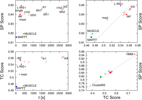
Performance measures for different aligners/command‐lines for BAliBASE3. Left‐hand panels show sum‐of‐pairs (SP) score on top or total column (TC) score at bottom against execution time. Right‐hand panels show SP vs TC score. Clustal Omega data points are shown in red (default with a solid bullet, single linkage guide‐tree with a cross, maximum likelihood guide‐tree with a star, various iteration schemes with circles, itr1 and itr2 are single and double iterations). The remaining Clustal Omega data points correspond to options where guide‐tree and HMM iterations are performed a different number of times. For example, t2h1 performs two guide‐tree iterations and one HMM iteration. MAFFT data points are shown in blue (default mode with solid bullet, L‐INS‐i mode with triangle). MUSCLE data point is in green. The bottom‐right panel contains the same data points as the top‐right panel, with two extra data points (ClustalW2 and HMM over‐training) added

Considering the SP score, averaged over all 218 families, and excluding Clustal Omega's external HMM option, MAFFT L‐INS‐i exhibits the highest score. ClustalW2, MAFFT default and MUSCLE deliver the lowest average SP scores, slightly outperformed by Clustal Omega default. With the exception of refining the guide‐tree twice but not using HMM information, all Clustal Omega iteration schemes perform better than the default option, with two outright iterations delivering the best average SP score, only marginally less accurate than MAFFT L‐INS‐i, but eight times as slow. The data suggest that guide‐tree refinement should not be performed more often than HMM iteration. There are also listed three nonstandard Clustal Omega options. The first uses as a guide‐tree the maximum likelihood tree derived from the reference alignment, calculated by FastTree‐2.21 This option delivers a poor result, which is unsurprising as it has been systematically shown for small alignments that phylogenetic trees do not make for good guide‐trees.22 The second option uses an externally generated single‐linkage tree as a guide‐tree. For small alignments, as in BAliBASE3 this option is of medium quality. The third nonstandard option uses an external HMM, which has been constructed from the reference alignment, using HMMER3.23 This, of course, is an unashamed exercise in over‐fitting, but has been included here to demonstrate the potential of using HMM background information. In terms of the average SP score this option almost recovers 100% of all residue pairs.

The overall picture is slightly different, when considering the TC score. Here all Clustal Omega default and iteration schemes perform better than MAFFT L‐INS‐i, which in turn is better than MUSCLE, MAFFT default and ClustalW2. Using a maximum likelihood tree still is a bad option and using an over‐trained HMM retrieves more than three quarters of all columns, delivering by far the highest average TC score.

Prefab

Results for Prefab follow a similar pattern as for BAliBASE. As can be seen in Figure 2, default MAFFT is the fastest program to align the 1682 families with on average 45 sequences. MAFFT L‐INS‐i, again is the aligner that achieves the highest average sum‐of‐pairs (SP) score. There are only two reference sequences in each Prefab alignment, therefore the SP score is the same as the total column (TC) score. The default version of Clustal Omega, again, strikes the optimum balance, being faster than MAFFT L‐INS‐i and more accurate than default MAFFT. All Clustal Omega iteration schemes deliver an improvement in the SP score; however, they increase the run time by a factor of two to six. The data point for ClustalW2 has been omitted from Figure 2, as its SP score is 0.06 lower than MUSCLE and its execution time twice as long. Constructing all distance matrices using Clustal Omega took around 2.5 minutes, constructing the single linkage trees less than ten seconds; so there is an overhead to the single linkage times of less than three minutes.

Figure 2.

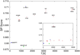
Performance measures for different aligners/command‐lines for Prefab, showing sum‐of‐pairs score versus execution time in seconds. The data point colors and symbols are the same as in Figure 1 (Clustal Omega red, MAFFT blue, MUSCLE green etc.). The main panel shows options without external HMM information. The small inset shows the same points as in the main panel with the one data point for external HMM added

HomFam

We selected three HomFam data sets to demonstrate how the execution time scales with the number of sequences. Error bars indicate the run times for the individual families. The lower edge of the bar corresponds to the time for the shortest family (zf‐CCHH), the top edge for the longest family (RuBisCO_large) and the solid data point between the upper and lower edge for the medium length family (rvp). One can see that for 100 sequences, default MAFFT is faster than default Clustal Omega and default MUSCLE. MUSCLE has a higher‐speed option, which employs a smaller number of refinements than the default (two as opposed to 16). For 100 sequences this option is faster than Clustal Omega, but still not as fast as default MAFFT. However, as the number of sequences is increased to around 2000, Clustal Omega overtakes the high speed MUSCLE version, and for around 10,000–20,000 sequences, overtakes default MAFFT. This is because computation times in Clustal Omega scale like Nlog(N), while for default MAFFT and both versions of MUSCLE they scale quadratically. In Figure 3, we fitted a power law to the data points for 1000 or more sequences. The exponent of this power law, given in brackets in the key, is a measure for the scalability. Small exponents correspond to a shallow curve in double‐logarithmic representation, and indicate good scalability; high exponents correspond to steeper curves and indicate poor scalability. MAFFT also has an option called PartTree, that scales basically like Nlog(N) and for this data set is faster than default Clustal Omega. However, alignments produced by this option are of lower quality than for default MAFFT or Clustal Omega (results not shown, but see, for example12). ClustalW2 and default MUSCLE exhibit similar quadratic scalability, being slower than Clustal Omega, while MAFFT L‐INS‐i is consistently the slowest aligner in this study. However, the exponent for MAFFT L‐INS‐i is 2.02, which is much smaller than would be expected for a consistency based high‐quality aligner.

Figure 3.

Execution times for different aligners/options as number of input sequences is changed. The color scheme is the same as in Figures 1 and 2 (Clustal Omega red, MAFFT blue, MUSCLE green, ClustalW2 orange). Solid bullets are used for default options: blue triangle for MAFFT L‐INS‐i, blue box for MAFFT PartTree, green box for fast MUSCLE option, orange circles for ClustalW2. Error bars indicate times for short (bottom), medium (middle) and long (top) protein domains. Solid lines connecting middle points are used to guide the eye

QuanTest

The QuanTest data set, used in this study, is comprised of 151 families of 1000 sequences, containing three reference sequences of known 3D structure, for which the correct alignments and secondary structures are known. The results are shown in Figure 4. Again, MAFFT default is the fastest aligner, taking on average less than 10 s for each alignment. The next fastest standard aligner is default Clustal Omega with an average time of about one minute. The slowest aligners are MUSCLE, ClustalW2 and Clustal Omega, using an externally generated single‐linkage tree. Single linkage trees tend to be more imbalanced than neighbor joining or UPGMA trees. It has long been recognized that Clustal Omega produces high quality alignments but slow response times when using highly imbalanced guide‐trees.20 MAFFT L‐INS‐i is roughly five times slower than default Clustal Omega. There is a small difference in the run times of default Clustal Omega and its full distance matrix option. Times for external tree options do not include times for construction of the trees.

Figure 4.

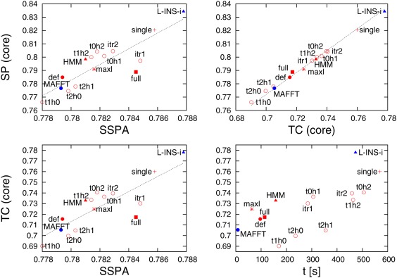
Performance measures for different aligners/command‐lines for QuanTest. Top‐left panel shows sum‐of‐pairs (SP) score versus secondary structure prediction accuracy (SSPA). Bottom‐left panel shows total column (TC) score versus SSPA score. Top‐right panel shows SP score versus TC score. Bottom‐right panel shows TC score versus execution time. Colour scheme and symbol shapes are the same as in Figures 1 and 2

In terms of the SP score, averaged over all 151 QuanTest families, MAFFT L‐INS‐i achieves the highest score, followed by Clustal Omega, using a single linkage tree. Again, iteration schemes, where the guide‐tree is refined more often than HMM background iteration, perform poorer than default Clustal Omega or its other iteration schemes. Using the full distance matrix delivers a marginally better average SP score than the Clustal Omega default option. For QuanTest, we do not have a standard reference alignment of all (in this case 1000) sequences. Therefore, a maximum likelihood tree cannot be derived from a reference alignment but is calculated from the default Clustal Omega alignment. Using this as a guide tree, we get an SP score that is only slightly better than Clustal Omega default but not worse, as for BAliBASE. This appears to justify using maximum likelihood trees as guide‐trees for large alignments but not for small ones. Equally, the background HMM is not over‐trained, like for BAliBASE, but is “off the shelf,” down‐loaded from Pfam. The SP scores vary by about 7% for the different Clustal Omega and MAFFT options.

The first thing to notice about the SSPA score is that it varies much less than the SP score, that is, by about 1% for the different Clustal Omega and MAFFT options. This variation grows to about 2% if ClustalW2 and MUSCLE are included. Unlike BAliBASE, the ranking of the different options is better preserved when switching from SP score to SSPA score (or TC score). The only noticeable exception being Clustal Omega's full distance matrix option, which moves from tenth best to fourth best in terms of SSPA score.

Memory and parallelization

In Figure 5, we show the CPU utilization and memory consumption, when aligning 20,000 HomFam sequences (Homstrad: p450; Pfam PF00067, Cytochromes P450; average length 329.9) on the 48‐core/256 GB platform. On the top row we show the utilization, when using six threads, on the bottom row the memory requirements. The left‐hand panels shows the initial phase of the MSA process, plotted against user time. User time measures the amount of work done by all threads together. The right‐hand panels show the entire alignment process, plotted against wall clock time, which is the actual time experienced by the person performing the alignment. Results for version 1.0.2 (2011) are shown in blue; results for the current version 1.2.3 (2016) are shown in red.

Figure 5.

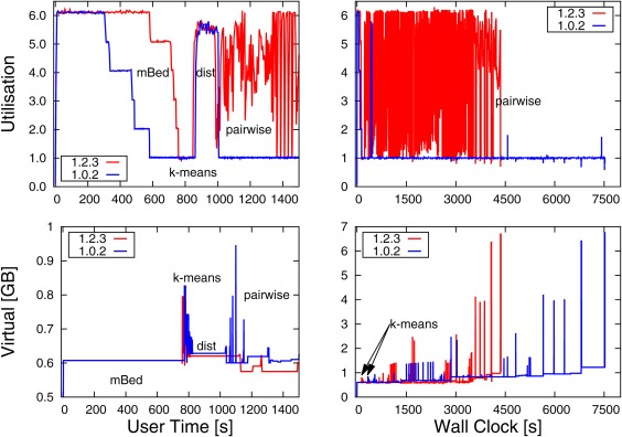
Resource requirements to align 20,000 p450 sequences, using default Clustal Omega. Top panels show utilization (out of 6 cores) when using six threads. Bottom panels show memory requirements. Left‐hand panels show requirements during initial alignment phase (pairwise distances and clustering), plotted against user time. Right‐hand panels show requirements during entire execution, plotted against wall clock time. Results for old Clustal Omega version 1.0.2 in blue, for current version 1.2.3 in red

The part of a progressive multiple aligner, that is easiest to parallelize, is the distance matrix calculation. The calculation of every distance between sequence pairs is completely independent from all the other distance pairs. Work can be effectively allocated at the beginning to different compute nodes, and the results can be easily combined at the end of the distance matrix calculation. This had already been implemented in version 1.0.2 of Clustal Omega1 and perfect load balancing was achieved for full distance mode, where the distance matrix is square. In default mBed mode, however, one does not calculate an all‐against‐all distance matrix but a distance matrix of all sequences against a small number of seed sequences. The distance matrix is therefore not square but oblong, with a large aspect ratio. However, the full matrix implementation was naively adapted to mBed mode, leading to imperfect load‐balancing. This can be seen in the top‐left panel. The process begins, after a negligible time for reading in the sequence data, with the mBed phase. Here the blue curve starts off with perfect utilization of 6 (given 6 threads). However, it then gradually decays until the k‐means phase begins at around 800 s of user time. The new 1.2.3 version (in red) maintains perfect utilization for longer, and only drops off, once the mBed phase has come to an end. The area between the blue and red curve during the mBed phase corresponds to a speed‐up in the actual running time. Memory consumption during the mBed phase is constant, as can be seen in the bottom‐left panel.

The next phase is the k‐means clustering. There, the sequences are clustered into groups of around 100 sequences. This phase has not been parallelized, and the utilization is 1. The bottom‐left memory panel shows a modest spike in memory consumption, which quickly decays, as the bi‐partitioning breaks down the clusters. However, this phase scales very unfavorably with the number of sequences. If, say, one million sequences were to be aligned, then this stage would be the bottle‐neck, consuming hundreds of GB of RAM (results not shown). Since the left‐hand panel are plotted against user time, which corresponds to the total amount of work being done by all threads, the red and blue segments for the k‐means memory requirements are congruent and are not shifted against each other as might have been expected due to the improved utilization of version 1.2.3 during the mBed phase.

During the final phase, full distance matrices are being calculated for each cluster, produced during the previous phase. Since the clusters are small, usually smaller than 100 sequences, utilization does not quite reach the maximum possible value of 6. Again, the red and blue curves for the small distance matrix calculation are congruent, because times are given in user time.

After the small distance matrix calculation follows the pairwise alignment phase. This phase had not been parallelized in version 1.0.2, and consequently the utilization is constantly 1 for the rest of the run‐time. This can be seen at the right edge of the top‐left panel but especially in the top‐right panel. Here the utilization is 1 for most of the time with two small blips at the left edge correspond to the mBed and small distance matrix calculation, described in the previous paragraphs. The red curve, however, shows utilization of greater than 1 for most of the time. This can be seen at the right edge of the top‐left panel but especially in the top‐right panel. The right‐hand panel is plotted against wall clock time, and one can see that the red curve giving results for version 1.2.3 terminates much earlier than the blue curve for version 1.0.2, reducing the over‐all time by roughly half. It should be noted that Clustal Omega by default tries to allocate all physically available compute nodes. This is not always necessary or desirable. On a busy machine, that is running other processes than Clustal Omega, this can lead to over‐threading, which may cause a dramatic increase in the response time. Also, due to Amdahl's law (law of diminishing returns), good speed‐up can be achieved for small numbers of threads, but very large numbers of threads are only useful for very large numbers of sequences.

The bottom‐right panel shows the memory consumption over the entire run‐time, plotted against wall clock time. At the very left edge one can see the exponentially decaying memory requests for the k‐means phase. These are displaced because the right‐hand panels show wall clock time. The displacement corresponds to the improved utilization due to improved load‐balancing of the mBed phase in version 1.2.3. The most noticeable feature of the bottom‐right memory panel is that the memory consumption during the pair‐wise alignment stage can soar to much higher values than during the distance matrix or clustering phase. Memory consumption during the initial phase is predominantly determined by the number of sequences. However, memory consumption during the pair‐wise alignment phase is exclusively determined by the lengths of the sequences and/or sub‐profiles to be aligned. In Clustal Omega's high accuracy MAC mode, one requires 48 times L1 times L2 bytes to perform an alignment, where L1 and L2 are the lengths of the two sequences or sub‐alignments to be aligned. In version 1.0.2 there were by default 2 GB available for MAC mode, which allowed to align two sequences or sub‐alignments that were each about 6500 residues long. In version 1.2.3 there are now 8 GB available to MAC by default. This allows us to align two sequences or sub‐alignments that are each about 13,000 residues long. While most protein sequences are shorter than 13,000 residues, large numbers of difficult to align sequences may incorporate many gaps, thereby inflating the total alignment size to well beyond the length of the longest unaligned sequence. In this case, Clustal Omega will switch from the high‐accuracy but memory hungry MAC mode to the lower‐quality but more memory‐frugal Viterbi mode. The point where this transition occurs can be specified by the user.

It is essential to note that all versions of Clustal Omega have always been thread‐safe. This means, that the alignment output does not depend on the number of threads used. Programs that are thread‐safe can create alignments in a reproducible manner. This is not the case if nonthread‐safe programs like MAFFT L‐INS‐i or PASTA are run with more than one thread. Here, every invocation may produce a different alignment, as the algorithm is inherently chaotic. If alignments have to be reproducible, then MAFFT L‐INS‐i or PASTA must be run using one thread only.

Discussion

Clustal Omega is now 8 years old and this paper is a convenient place to describe updates and to explore the accuracy of some of the iteration options that are provided. These options were described in the original paper but never explored in any detail. Here, we can see trade‐offs between speed and accuracy for some options and these are compared to some alternative MSA packages.

Over the past 8 years, the code of Clustal Omega has been maintained and numerous bug fixes dealt with. We have also added new functionality, often as a result from feedback from users. The most obvious of these is support for nucleotide sequences but we have also added a range of extra input and output features, including the ability to read zipped files and multi byte characters in sequence names. New output features include printing of residue numbers and control of line lengths and sequence order. Clustal Omega run times scale well with numbers of sequences. This is due to the use of the mBed algorithm for guide trees as well as parallelization of the distance matrix calculation to use multiple threads. The progressive phase has also now been partially parallelized, giving further scalability, especially for large numbers of sequences.

In terms of measuring accuracy, we have used three benchmarks, based on protein structural similarity. These were BALiBASE and Prefab which use relatively small alignments that have been carefully curated and QuanTest which is automatically generated and can realistically test large alignments. With BALiBASE, default Clustal Omega is almost as good as MAFFT L‐INS‐i in terms of SP score but better in terms of TC score. MAFFT L‐INS‐i is designed for very accurate alignment of just a few hundred sequences. It uses a consistency based algorithm, like that in the original T‐Coffee program. The QuanTest benchmark alignments we use, all have embedded sequences with known structure. These are used to test secondary structure prediction accuracy as a proxy for alignment accuracy; the alignments are used to predict secondary structure and the predicted structures are compared to the known ones. The alignment of the embedded reference sequences can also be used to test alignment accuracy by comparing their alignment to a structure based alignment, with TC and SP scores. Here, the QuanTest and SP/TC scores agree well but the QuanTest benchmarks are easier to generate fully automatically and properly test the alignment of all the sequences, not just the references.

All of the iteration schemes improve alignment quality but at the expense of run‐times. There is tremendous potential to use the external HMM facility to improve accuracy. Here, we use an existing profile HMM of sequences that are homologous to the input sequences. Then, each sequence is aligned to the HMM and residue pseudo counts are taken from the HMM and transferred, position by position to the sequences to be aligned. It is a way to use existing alignment information. These profile HMMs can be generated locally from a curated alignment or taken from HMM repositories such as Pfam.

Finally, we notice a great deal of variation in accuracy, depending on the algorithms used to generate the guide trees. These algorithms vary enormously in terms of algorithmic complexity. In a worst case scenario we would like to point out that some supposedly rigorous methods for calculating pair‐wise distances and clustering can give the worst of both worlds: slow run times and poor alignments. This is an area that has great potential for further improvements.

References

- 1. Sievers F, Wilm A, Dineen D, Gibson TJ, Karplus K, Li W, Lopez R, McWilliam H, Remmert M, Soeding J, Thompson JD, Higgins DG (2011) Fast, scalable generation of high‐quality protein multiple sequence alignments using Clustal Omega. Mol Syst Biol 7:539. [DOI] [PMC free article] [PubMed] [Google Scholar]
- 2. Thompson JD, Higgins DG, Gibson TJ (1994) CLUSTAL W: improving the sensitivity of progressive multiple sequence alignment through sequence weighting, position‐specific gap penalties and weight matrix choice. Nucleic Acids Res 22:4673–4680. [DOI] [PMC free article] [PubMed] [Google Scholar]
- 3. Thompson JD, Gibson TJ, Plewniak F, Jeanmougin F, Higgins DG (1997) The CLUSTAL_X windows interface: flexible strategies for multiple sequence alignment aided by quality analysis tools. Nucleic Acids Res 25:4876–4882. [DOI] [PMC free article] [PubMed] [Google Scholar]
- 4. Edgar RC (2004) MUSCLE: multiple sequence alignment with high accuracy and high throughput. Nucleic Acids Res 32:1792–1797. [DOI] [PMC free article] [PubMed] [Google Scholar]
- 5. Katoh K, Kazuharu M, Kuma K, Miyata T (2002) MAFFT: a novel method for rapid multiple sequence alignment based on fast Fourier transform. Nucleic Acids Res 30:3059–3066. [DOI] [PMC free article] [PubMed] [Google Scholar]
- 6. Notredame C, Higgins DG, Heringa J (2000) T‐Coffee: A novel method for multiple sequence alignments. J Mol Biol 302:205–217. [DOI] [PubMed] [Google Scholar]
- 7. Katoh K, Kuma K, Toh H, Miyata T (2005) MAFFT version 5: improvement in accuracy of multiple sequence alignment. Nucleic Acids Res 33:511–518. [DOI] [PMC free article] [PubMed] [Google Scholar]
- 8. Higgins DG, Bleasby AJ, Fuchs R (1992) CLUSTAL V: improved software for multiple sequence alignment. Comput Appl Biosci 8:189–191. [DOI] [PubMed] [Google Scholar]
- 9. Sankoff D, Morel C, Cedergen RJ (1973) Evolution of 5S RNA and the non‐randomness of base replacement. Nature 245:232–234. [DOI] [PubMed] [Google Scholar]
- 10. Blackshields G, Sievers F, Shi W, Wilm A, Higgins DG (2010) Sequence embedding for fast construction of guide trees for multiple sequence alignment. Algorithms Mol Biol 5:21. [DOI] [PMC free article] [PubMed] [Google Scholar]
- 11. Söding J (2005) Protein homology detection by HMM‐HMM comparison. Bioinformatics 21:951–960. [DOI] [PubMed] [Google Scholar]
- 12. Le Q, Sievers F, Higgins DG (2017) Protein multiple sequence alignment benchmarking through secondary structure prediction. Bioinformatics 33:1331–1337. [DOI] [PMC free article] [PubMed] [Google Scholar]
- 13. Thompson JD, Plewniak F, Poch O (1999) A comprehensive comparison of multiple sequence alignment programs. Nucleic Acids Res 27:2682–2690. [DOI] [PMC free article] [PubMed] [Google Scholar]
- 14. Thompson JD, Koehl P, Ripp R, Poch O (2005) BAliBASE 3.0: latest developments of the multiple sequence alignment benchmark. Proteins 61:127–136. [DOI] [PubMed] [Google Scholar]
- 15. Mizuguchi K, Deane CM, Blundell TL, Overington JP (1998) HOMSTRAD: a database of protein structure alignments for homologous families. Protein Sci 7:2469–2471. [DOI] [PMC free article] [PubMed] [Google Scholar]
- 16. Finn RD, Bateman A, Clements J, Coggill P, Eberhardt RY, Eddy SR, Heger A, Hetherington K, Holm L, Mistry J, Sonnhammer EL, Tate J, Punta M (2014) Pfam: the protein families database. Nucleic Acids Res 42:D222–D230. [DOI] [PMC free article] [PubMed] [Google Scholar]
- 17. Fox G, Sievers F, Higgins DG (2016) Using de novo protein structure predictions to measure the quality of very large multiple sequence alignments. Bioinformatics 32:814–820. [DOI] [PMC free article] [PubMed] [Google Scholar]
- 18. Drozdetskiy A, Cole C, Procter J, Barton GJ (2015) JPred4: a protein secondary structure prediction server. Nucleic Acids Res 43:W389–W394. [DOI] [PMC free article] [PubMed] [Google Scholar]
- 19. Gardner PP, Wilm A, Washietl S (2005) A benchmark of multiple sequence alignment programs upon structural RNAs. Nucleic Acids Res 33:2433–2439. [DOI] [PMC free article] [PubMed] [Google Scholar]
- 20. Boyce K, Sievers F, Higgins DG (2014) Simple chained guide trees give high‐quality protein multiple sequence alignments. Proc Natl Acad Sci USA 111:10556–10561. [DOI] [PMC free article] [PubMed] [Google Scholar]
- 21. Price MN, Dehal PS, Arkin AP (2010) FastTree 2–approximately maximum‐likelihood trees for large alignments. PLoS One 5:e9490. [DOI] [PMC free article] [PubMed] [Google Scholar]
- 22. Sievers F, Hughes GM, Higgins DG (2014) Systematic exploration of guide‐tree topology effects for small protein alignments. BMC Bioinform 15:338. [DOI] [PMC free article] [PubMed] [Google Scholar]
- 23. Finn RD, Clements J, Eddy SR (2011) HMMER web server: interactive sequence similarity searching. Nucleic Acids Res 39:W29–W37. [DOI] [PMC free article] [PubMed] [Google Scholar]