

Abstract
Xplor‐NIH is a popular software package for biomolecular structure determination from nuclear magnetic resonance (NMR) and other data sources. Here, some of Xplor‐NIH's most useful data‐associated energy terms are reviewed, including newer alternative options for using residual dipolar coupling data in structure calculations. Further, we discuss new developments in the implementation of strict symmetry for the calculation of symmetric homo‐oligomers, and in the representation of the system as an ensemble of structures to account for motional effects. Finally, the different available force fields are presented, among other Xplor‐NIH capabilities.
Keywords: structure determination, NMR restraints, SAXS, cryo‐electron microscopy, optimization, computational toolbox, protein, nucleic acid
Introduction
Xplor‐NIH1 is a software package for biomolecular structure determination from various experimental data sources combined with known geometric data. Structure determination is achieved by seeking the minimum of a target energy function comprising terms for the experimental restraints, covalent geometry and non‐bonded contacts using a variety of optimization procedures such as molecular dynamics in Cartesian and torsion angle space, Monte Carlo methods and conventional gradient‐based minimization.
Xplor‐NIH was originally derived from XPLOR2 version 3.851 and contains all of the functionality therein. While this legacy component is supported and readily accessed, a completely reworked framework with a Python scripting language front end has been the basis of development for the past 15 or so years.
Xplor‐NIH is written in a combination of languages, with the older XPLOR interface coded in Fortran 77. This component corresponds closely to XPLOR 3.851, with some additions, bug fixes and enhancements. One major change to the Fortran code was the removal of all structure‐based limits, so that the maximum number of atom, bonds, and so forth, is now determined by the amount of the computer's random access memory (RAM), and not by precompiled constants. Most recent computationally intensive code has been developed in the C++ language, with interfaces to the Python and Tcl scripting languages generated automatically with the SWIG package.3 Most of Xplor‐NIH's code is now being developed directly in the Python language, and thus is directly accessible for modification by the end‐user without recompilation, while code paths which require high performance, such as those executed at every timestep of molecular dynamics, are coded in C++. The Python interface to Xplor‐NIH provides an extensible toolbox for developing further functionality. Precompiled packages for most popular Unix and Unix‐like operating systems (such as Linux and Mac OS X), as well as documentation and support are available directly from http://nmr.cit.nih.gov/xplor-nih/. The full source code package is available by email request to requests@nmr.cit.nih.gov. Xplor‐NIH is freely available (in both source and executable formats) for research purposes. For commercial use of Xplor‐NIH, contact C.D.S.
Xplor‐NIH is a collaborative effort, with groups worldwide contributing advice and computer code. Additional contributions are particularly encouraged as these are advantageous to the contributors as well as to other end‐users. New contributions should adhere to Xplor‐NIH coding conventions, and be accompanied by appropriate testing scripts to assure reproducible future operation.
This article provides an overview of the current state of Xplor‐NIH, and references an earlier review4 where features have not changed. The previous general description of Xplor‐NIH was published 11 years ago,4 and this work documents the significant changes and enhancements which have been implemented since then.
Here we assume some familiarity with the Python language as example code is included throughout. For a good introduction to the language see Ref. 5. This article is organized as follows. The following Section presents a brief introduction to the Python interface. This is followed by an introduction to some of the most often used energy terms in structure determination, along with Python example code. The next Section details commonly used force fields. This is followed by an overview of Xplor‐NIH's new strict symmetry facility, and then an update on the use of facilities for ensemble refinement, including population optimization. The following Section covers new standard data formats supported by Xplor‐NIH. The final Section presents other Xplor‐NIH facilities, including external helper programs.
Overview of the Python Interface
In the most common use of Xplor‐NIH, an energy metric is minimized by a combination of simulated annealing using molecular dynamics, and gradient minimization. The energy metric is a sum of terms corresponding to experimental, chemical and knowledge‐based restraints. Experimental restraints include traditional NMR restraints, such as those based on interatomic distances obtained from Nuclear Overhauser Effect (NOE) experiments, and torsion angles, obtained from chemical shifts or scalar coupling data. Chemical restraints consist of those corresponding to covalent geometry and a desire to prevent atomic overlap. Knowledge‐based terms restrain structures based on statistical trends seen in a database of structures, an example of which is an energy term which biases torsion angles to regions of dihedral angle space that are populated by well‐defined regions in high‐quality crystal structures.
Atomic properties such as Cartesian coordinates, atom names, masses, and so forth are contained in a Simulation object. The default Simulation is a xplorSimulation.XplorSimulation object which can be accessed as xplor.simulation. The coordinates in xplor.simulation are mirrored in the XPLOR interface. A separate set of atomic properties can be created by instantiating a new XplorSimulation object, which will be associated with a separate Unix process. For instance, an extra XplorSimulation object can be useful for holding coordinates of a homologous structure for comparison or to be used as a restraint. Other simulations are used with ensemble and strict symmetry calculations as described below. Direct access to atomic properties can be obtained via methods of a simulation object, or using an atomSel.AtomSel object. Commands in the old XPLOR language can be executed by calling the command method of xplor.simulation.
The atom selection language is almost identical to that in the XPLOR interface and is documented in the atomSelLang module. Additions to the selection language include the INDEx keyword which allows one to reference atoms by their internal 0‐offset reference number, the PSEUdo keyword which selects all pseudo atoms, and the RECAll keyword which allows one to reference by name an atom selection previously defined by the atomSelLang.setNamedSelection function.
Atomic coordinates can be read and written using a pdbTool.PDBTool object, but in most scripts, higher level functions perform this function. For instance, coordinates are most often read using protocol.initCoords or protocol.loadPDB, which also understand how to convert atom names from different schemes to those used in Xplor‐NIH. Coordinates are most easily written using the protocol.writePDB function, or by the automatic facilities provided by simulationTools.StructureLoop. Torsion angles can be set to nominal values from a XPLOR‐formatted restraint table using the torsionTools.setTorsionsFromTable function. On the other hand, the monteCarlo.randomizeTorsions function can be used to randomize all torsion angles active in a particular IVM object.
By convention, Xplor‐NIH energy terms exist in Python modules with the suffix PotTools. So, for instance, the terms for distance restraints and residual dipolar couplings (RDCs) are in the modules noePotTools and rdcPotTools, respectively. In these modules, the functions that create the energy terms take the prefix create_, so that the creation functions corresponding to the above terms are create_NOEPot and create_RDCPot, respectively. On the other hand, energy terms defined in the legacy XPLOR interface are instantiated via the XplorPot constructor function from the xplorPot module. XplorPot energies typically used in modern Xplor‐NIH scripts include BOND, ANGL and IMPR, the covalent energy terms for bonds, angles and improper dihedral angles, respectively, and CDIH, the energy term which restrains dihedral angles to experimentally determined values. There are helper functions in the protocol module to help initialize and configure commonly used XPLOR terms, where appropriate.
The internal variable module (IVM)6 is used to manipulate coordinates either by molecular dynamics or gradient minimization. This facility allows generalized internal coordinates ranging from the three degrees of freedom per atom in Cartesian coordinates to torsion angle space, to allowing rigid‐body motions of arbitrarily large subunits. IVM objects can be created by the ivm.IVM constructor and the desired degrees of freedom then specified. The final step in the topology setup of an IVM object should be a call to either of the helper functions protocol.torsionTopology or protocol.cartesianTopology. These functions configure those degrees of freedom not already specified, for either torsion or Cartesian degrees of freedom, respectively. torsionTopology groups in rigid bodies atoms in aromatic and other known planar regions. Its use is demonstrated in Figure 1. In addition, these functions take care of proper configuration of pseudo atoms, used to encode non‐atomic coordinates such as those atoms which describe the RDC alignment tensor, and those which encode ensemble populations (see below). IVM objects are configured for dynamics or minimization by use of the protocol.initDynamics or protocol.initMinimize functions, respectively.
Figure 1.
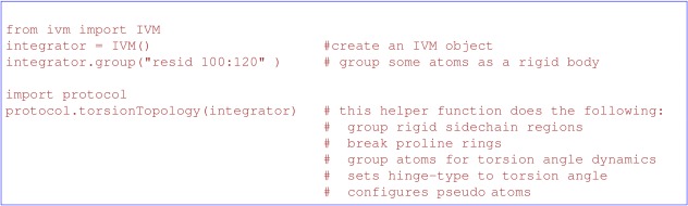
Topology setup for torsion angle dynamics with a grouped region composed of residues numbered from 100 to 120, inclusive.
As described above, functions used to configure standard settings for dynamics, minimization and XPLOR energy terms can be found in the protocol module. For example, to load a protein structure file (PSF) (which contains atom information and covalent geometry definitions for a particular structure, used for proteins and all other types of molecules), the initStruct function can be used as seen in Figure 2. Figure 2 also shows that PSF information can also be directly generated from a residue sequence using functions in the psfGen module. Alternatively, for proteins and nucleic acids containing standard residues, protocol.loadPDB can be used to generate PSF information directly from a PDB or mmCIF file, and the coordinates then loaded. [loadPDB can also optionally generate subunits related by crystallographic symmetry from a PDB BIOMT record.]
Figure 2.
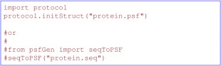
Loading PSF information from a file, or generating it from sequence. protein.psf would contain a pre‐calculated PSF file, while protein.seq would contain a list of whitespace‐separated 3‐character residue names. PSF information is required for any Xplor‐NIH functionality which references atomic coordinates.
An outline of a complete structure calculation script can be found in Figure 3, which introduces AnnealIVM, used to perform simulated annealing, and StructureLoop, which repeatedly calls a function to compute the requested number of structures (optionally in parallel) and then writes out the coordinates.
Figure 3.
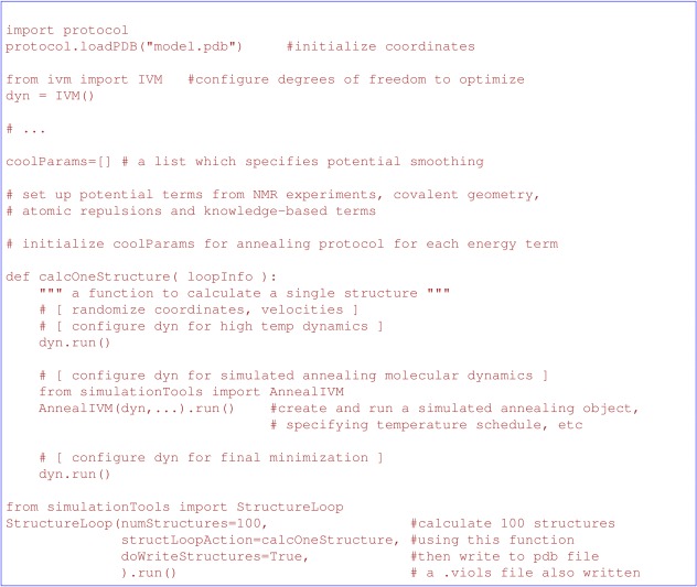
Schematic of a structure calculation script.
The Python interpreter is invoked via the xplor ‐py or pyXplor commands. In Xplor‐NIH's Python interface, functions and class definitions are placed in module namespaces; a reference manual for all Xplor‐NIH modules is available.7 The Python built‐in function help can be used to get immediate help about Python objects. The following conventions are used in Xplor‐NIH's Python interface: module and function names start with lower‐case letters and class names start with upper‐case letters.
While the primary interface for Xplor‐NIH is via Python, the legacy XPLOR interface continues to be maintained, and can be utilized for additional functionality not yet supported by the Python interface, such as refinement against X‐ray crystallographic or fiber data. Xplor‐NIH's Tcl interface is used solely for the PASD8 automatic NOE assignment facility. Xplor‐NIH ships with multiple additional facilities including the numpy9 and matplotlib10 packages.
Options for parallel structure calculation
To ascertain the range of conformations consistent with the experimental restraints and other energy terms, multiple structures are usually computed which differ in the random number seed used for generation of initial random coordinates and velocities. Additionally, it is common that some structures will fail to converge to an acceptable solution, so running multiple calculations increases the chance of success. For a production refinement calculation, it is common to compute 100 or more structures.
On a workstation with multiple cores, one may specify the ‐smp command line option to run structure calculations in parallel. Similarly, on Scyld ClusterWare systems, one specifies ‐scyld . Xplor‐NIH also supports clusters running the PBS11 or SLURM12 queuing software using the pbsxplor and slurmXplor commands, respectively. These commands will create a job submission script appropriate for the queuing system, and help assure that Xplor‐NIH is run efficiently on each node of the cluster. For example, with pbsxplor, the number of cluster nodes N is specified with the ‐l nodes= N option, and is then automatically computed.
Energy Terms
Xplor‐NIH energy terms can be divided into four general classes:
Terms that reflect how well experimental observables are predicted from the molecular structure. Examples of NMR terms include those that enforce NOE and RDC restraints. Examples of non‐NMR data terms are those from small angle solution scattering (SASS),13 cryo‐electron microscopy (cryo‐EM),14 and X‐ray crystallography.15, 16, 17
Those terms which enforce covalent geometry and prevent bad atom–atom contacts. Example terms include bond, angle, improper dihedral, and non‐bonded terms.
Statistical or knowledge‐based energy terms derived from the Protein Data Bank which bias structures towards existing features seen in the database. An example is the torsionDB multi‐dimensional torsion angle database energy term.18, 19 When these terms are designed, special care is taken so that they are readily overridden by experimental restraints in cases of conflict.
Other energy terms used to aid with structure determination—generally to aid with convergence or to enforce other physical information gleaned about the structure. For example, such terms include XPLOR's NCS and HARM terms, which enforces symmetry, and restrains atomic positions, respectively.
Ideally, only the first class of energy terms would be necessary in structure determination, but the problem is underdetermined, such that experimental restraints alone usually do not contain sufficient structural information.
Standard energy terms
Energy terms for various NMR experiments are listed here. The following energy terms are implemented in the modern Python/C++ interface:
The previously mentioned NOEPot term is usually used for distance restraints. This term supports the XPLOR ASSIgn OR format to provide pairs of ambiguous assignments, and different averaging options such as sum averaging.20 This term supports the standard piece‐wise quadratic,4 log‐normal,21 and soft forms of the energy function.
The RDCPot term can be used for RDC restraints, as well as dipolar coupling restraints from solid state NMR. It allows one to choose the flexibility of the alignment tensor, from being fully fixed to allowing all five degrees of freedom. One can treat through‐space RDCs by enabling the distance dependence of this term by setting the useDistance accessor. This form of the energy term thus also supports pseudo‐contact shift restraints.
Chemical shift anisotropy can be measured in solid state NMR and using weakly aligning media in solution.22 These data can be used as restraints on bond vector orientation using the CSAPot term.
Restraints on torsion angles from three‐bond J coupling experiments are supported by the JCoupPot term.4
DiffPot 23 is an energy term restraining the shape of a protein using components of the rotation diffusion tensor extracted from NMR relaxation data.
Direct use of ratios from relaxation data is afforded by the RelaxRatioPot term to provide information on overall molecular shape and local bond vector orientations in docking24 and all‐atom structure determination.25
Refinement against cross‐correlation relaxation (CCR) can be performed using CCRPot.26 This term is only meaningful in the context of an EnsembleSimulation.
Solvent NOE and PRE data can be qualitatively incorporated into structure calculations using the NBTargetPot term.27
The OrderPot term can be used to refine against bond angle S 2 parameters. This term is only meaningful in the context of an EnsembleSimulation.
Paramagnetic relaxation enhancement (PRE) can be used to derive long‐range (10–30 Å) distance information via the Solomon–Bloembergen equation. While PREs are sometimes converted to distance restraints, Xplor‐NIH supports structure calculation directly from PRE values with the PREPot term,28 and includes an extension which better describes motional effects due to flexibly‐linked paramagnetic groups. Because of the distance dependence of PREs, these are powerful in characterizing minor populations of a species in the case where there are distances in the minor species which are smaller than the corresponding distances in the major species.29
Experimentally measured scalar coupling values30, 31 can be fit to single structures using the h3JNCPot energy term to provide an empirical measure of the quality of hydrogen bond geometries.
Certain possibly useful NMR energy terms in the old XPLOR interface are listed next:
Torsion angle restraints32 derived from three‐bond J couplings in combination with NOE/ROE data are available in the CDIH XPLOR energy term accessed via the RESTraints DIHEdral XPLOR statement.
The couplings are related to ϕ and ψ angles by an empirical relationship.33 coupling restraints are available via the ONEBond XPLOR term (J.J. Kuszewski and G.M.C., unpublished).
/ secondary shifts,34 which are empirically related to ϕ/ψ values,35 are available in the CARBon XPLOR term.
1H chemical shifts restraints,36, 37 which include the capability of dealing with nonstereospecifically assigned methylene and methyl groups are available in the PROTon XPLOR term.
Direct refinement against NOE intensities using complete relaxation matrix calculations38, 39 are available via the RELAxation XPLOR term. This approach is computationally intensive, and for this reason is used infrequently and then only in the very last stages of a refinement protocol.
Heteronuclear ratios for molecules that tumble anisotropically40, 41 also provide orientational information. Associated restraints can be applied using the DANI XPLOR term.
Alternative RDC energy terms are available. The Implicit Saupe tensor Alignment Constraint (ISAC)42 code available via the XPLOR TENS energy term allows for a floating orientational tensor without explicit tensor atoms. The VEAN term43 imposes intramolecular angle restraints derived from RDCs in a smooth energy term which can be useful for early stages of refinement. The VEAN term is also useful to apply restraints from tensor‐based solid state NMR experiments in structure calculations.44
In addition to torsionDB (discussed further below) other knowledge‐based terms derived from the Protein Data Bank (PDB) are also available. Backbone amide hydrogen bonding is encoded via two terms. The HBDA XPLOR term45 employs an empirical relationship between hydrogen‐oxygen distance and the NHO angle. An alternative representation of backbone hydrogen bonding is encoded in the HBDB XPLOR term,46 which is a direct potential of mean force.
The ORIE XPLOR energy term comprises another database term containing information about the relative positioning of groups close in space. The term currently encodes base‐base information for DNA47 and RNA,48 as well as protein sidechain‐sidechain interactions (J.J. Kuszewski and G.M.C., unpublished). For nucleic acids, use of this term leads to a significant increase in accuracy as judged by cross‐validation against dipolar couplings and circumvents limitations associated with conventional NMR representations of non‐bonded contacts. The term's usefulness was underscored by comparison of high‐angle X‐ray scattering data with the calculated structures of a double‐stranded DNA dodecamer.49
The gyration volume50 and radius of gyration51 energy terms are useful to obtain structures with approximately correct atomic density. These restraints can be applied to well‐packed ellipsoidal regions of protein structures using the create_GyrPot and create_RgyrPot functions from the gyrPotTools modules. residueAffPot 23 implements a per‐residue packing potential energy which encodes the arrangement of hydrophobic, polar and charged residues.
New energy terms can be written purely in Python. Thus, new terms can be prototyped rapidly. If execution speed requires, such a term can later be recoded in C++, with no change to the structure calculation scripts.
New RDC terms
Aside from the standard Xplor‐NIH RDC energy term,4 we have implemented two additional terms which are particularly useful for ensemble calculations. For interconversion fast on the RDC timescale, each ensemble member has its own effective alignment tensor, and if one were to use the common practice of letting the alignment tensors float to optimize fit to experiment, there would be far too many parameters for the given data.
SARDC
The SARDC energy term52 computes the alignment tensor from molecular shape, which is appropriate for experiments performed using purely steric alignment media. After initial publication, the SARDC term was updated and corrected.53 Corrections included proper calculation of the gradient with respect to the alignment tensor. Updates included adding support for pairwise averaging such that a single restraint table can simultaneously be used for symmetric homodimers and the monomeric species.
The target function for the SARDC term is proportional to the metric:
| (1) |
where δ i is the calculated RDC value for residue i, is the observed experimental value, is an error, and the sum extends over all NRDC observed RDCs. Errors arise from experiment and due to coordinate error.
While the alignment tensor is computed from the structure, there remains an overall scale factor which is chosen to optimize the fit to experiment. RDCs from multiple experiments can be combined to use a shared tensor. They can be read as a single set, or placed in separate terms for convenience, but in the later case they must be linked so that they share the overall RDC scale factor.
RDCCorrPot
An alternative approach for treating RDCs in an ensemble calculation is to compute RDCs from structure using a tensor‐less approach.54 Here, the proper overall RDC scale factor is again unknown, so the default target function is , the correlation of observed to calculated RDCs:
| (2) |
where and are the average of the calculated and observed RDC values, respectively. For this term, the usual form for the energy is
| (3) |
where k RDC is a force constant. The rdcCorrPotTools.calibrate function can be used to compute the appropriate scale factor so that RDC values can be compared, and (optionally) a “harmonic” potential energy type then used to restrain individual restraints.
Non‐NMR energy terms
In addition to the full set of facilities for refining against X‐ray crystallographic2 and X‐ray fiber diffraction data55 implemented in the XPLOR interface, we implemented two sets of facilities for which increasing amounts of data are now available.
SASS data
Small angle X‐ray scattering (SAXS) and small‐angle neutron scattering (SANS) can be used to study samples under conditions very similar to those of NMR. As these data are sensitive to overall size and shape information, they are complementary to NMR data. A detailed review of Xplor‐NIH's SASS facilities has been reported13 and the reader is directed there for a description and for Python snippets to use for incorporating SASS data into an existing script. The SASS terms are implemented in solnScatPot.SolnScatPot terms created by create_ functions in the modules solnXRayPotTools and sansPotTools.
Cryo‐EM maps
Xplor‐NIH has a native OpenMP‐parallelized facility to handle cryo‐EM density maps.14 Recent advances in cryo‐EM technology has enabled the technique to achieve nearly atomic resolution. An example snippet for using cryo‐EM data in structure determination can be found in Figure 4.
Figure 4.
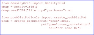
Setup of the energy term for refining against an atomic probability density map (e.g., generated from cryo‐electron microscopy).
Force Fields
The force field describes molecular motion in the absence of experimental restraints. Xplor‐NIH can support and is shipped with multiple force fields, the choice of which can be tailored for one's particular need.
The default force field
The default force field includes bonds and angles designed to agree with the Engh and Huber parameter set56 for proteins and those of Parkinson et al.57 for nucleic acids, with improper dihedral angles used to uniquely define tetrahedral centers and to restrain rigid regions, such as aromatic rings. Dihedral angles are restrained using TorsionDBPot,18, 19 a multi‐dimensional knowledge‐based potential of mean force derived from high‐quality structures from the PDB. TorsionDB is an improvement over the earlier RAMA term,58, 59 and completely supersedes it. TorsionDB applies to proteins, RNA and DNA.
The default nonbonded term RepelPot is a simple excluded volume term which is a re‐implementation of the XPLOR VDW REPEl term.60 RepelPot implements only the purely quartic repulsive term, but allows more convenient specification of which atoms are included or excluded, and has been efficiently OpenMP‐parallelized. With older force fields, the atomic radii were modified by a scale factor during simulated annealing. With the adoption of Molprobity radii,19 a single constant scale factor of 0.9 is now applied during simulated annealing. An example of typical RepelPot setup is shown in Figure 5.
Figure 5.
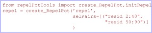
Setup of the RepelPot energy term for atom‐atom repulsion with the correct radius scale factor set automatically. This setup specifies that only interactions between residues 2–40 and 50–90 are computed. This setting can speed up non‐bonded calculations when regions are grouped as rigid bodies.
By default, the RepelPot setup excludes non‐bonded interactions between atoms separated by three or fewer bonds (i.e., 1–4 interactions) because most such interactions are implied by the torsionDB term. However, since the torsionDB term is derived from X‐ray structures, it only involves torsion angles defined by heavy atoms. Thus, torsion angles involved in methyl and O‐H group rotations are not restrained, which may lead to eclipsed conformations unless 1–4 non‐bonded interactions are introduced for these groups (e.g., between the H and C in serine residues). A separate RepelPot instance must be configured for this purpose, as shown in Figure 6.
Figure 6.
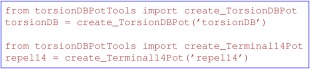
Instantiating the dihedral portion of the default force field using TorsionDBPot and Terminal14Pot for dihedral angles which contain one or more protons (see text).
EEFx
It has been noted that refinement of NMR structures in fully realistic force fields including electrostatics and the effects of solvent can improve NMR structures.61 Thus, an implementation of the EEF162 implicit solvent force field has been introduced into Xplor‐NIH as the EEFx term.63 While there is a modest slow down in computation time, this force field has been shown to be usable in all stages of structure determination, and can provide improvements over the results from the default RepelPot‐based force field.
The EEFx term also contains an implicit representation of lipid bilayer membranes,64 in which the dielectric constant modulates from that of bulk water at the membrane surface, to that appropriate for the lipid interior. This term has been shown to help determine the overall orientation of a membrane protein, and can help exclude hydrophilic regions from the membrane.
Figure 7 shows how the EEFx energy term is added to an Xplor‐NIH Python script. This term includes van der Waals, electrostatic and solvent contributions. It can be used in concert with either TorsionDBPot or the standard XPLOR DIHE dihedral term using CHARMM22 parameters.65
Figure 7.
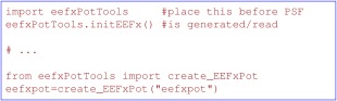
An example of how to include the EEFx energy term. The initEEFx function loads the appropriate electrostatic, non‐bonded and solvation parameters, while the eefxpot object is instantiated later in a script with other energy terms.
Alternate force fields
In addition to the EEFx term, Xplor‐NIH ships with support for the explicit water refinement protocol introduced in Ref. 66. Force field parameters may be easily modified by end‐users so as to ensure very small deviations from idealized covalent geometry, while satisfying experimental restraints and achieving good non‐bonded contacts (i.e., no atomic overlaps). Full empirical energy functions (CHARMM19/20/22, OPLS67) are also available. Finally, it is straightforward to adapt parameter and topology files for any empirical energy function (e.g., AMBER,68 etc.) which employs the same analytic form for the electrostatics, hydrogen bonding and van der Waals Lennard–Jones energy terms as CHARMM19/20. Note that obtaining parameters and topology information for other systems, including polysaccharides and small molecules, is relatively simple. Non‐proton information can be generated from arbitrary molecular coordinates using the Dundee PRODRG2 Server,69 XPLO2D,70 program, or ACPYPE.71 Frequently, some amount of manual editing of the generated topology and parameter data is required. If coordinates are known, the LEARn facility in the XPLOR interface can be used to generate the parameters.
Strict Symmetry
While approximate symmetry can be maintained using the terms PosDiffPot (which restrains atomic coordinates in different subunits to have the same relative configurations) and DistSymmPot (which implements distance symmetry20), Xplor‐NIH also has a strict symmetry facility implemented in the symSimulation module, in which only a single copy of protomer1 coordinates are maintained, and the other subunits are generated by rigid body rotations and translations.72 The advantages of this strict symmetry representation are that the number of coordinates are reduced by a factor of the size of the oligomer, and that only a subset of interactions need be computed, leading to faster sampling and reduced computational cost. See Figure 8 for an example of a symSimulation setup appropriate for a symmetric homodimer. All of the native Python energy terms can be applied to the full oligomer, or to the protomer alone, as is appropriate, while the old XPLOR terms have the limitation of only applying to the protomer. For example, torsion angle restraints only need be applied to the protomer, while intersubunit restraints would need be applied to the full SymSimulation. When setting up energy terms or IVM objects, the current Simulation is used unless otherwise specified. Hence, in strict symmetry calculations it is convenient to switch the current Simulation between the initial XplorSimulation containing protomer coordinates, and the SymSimulation which contains coordinates of the full construct using the function simulation.setCurrentSimulation. Strict symmetry has not yet been implemented in the EnsembleSimulation facility.
Figure 8.
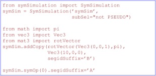
Example of generating a second subunit related by a rotation about the z axis relative to the protomer. The segment name of the second subunit is set to “B” while that of the first subunit is set to “A”.
Unlike the normal circumstance where the center of mass location is irrelevant, in strict symmetry calculations, the protomer center of mass location can encode subunit translational distances such as that involved in intersubunit packing. Normally, the center of mass velocities are zeroed at each time step for trajectory stability, but in strict symmetry calculations, one should allow some of this motion through a call to the setResetCMInterval method of IVM objects after a call to protocol.initDynamics so that different packing distances can be sampled during molecular dynamics.
A novel aspect of this strict symmetry implementation is the ability to optimize symmetry operations on the fly, for cases in which the rigid body rotations or translations are not known. For instance, for a molecule with helical symmetry, the amount and/or direction of helical twist can be allowed to float during structure calculations. Floating rotation and translation parameters are encoded in pseudo atoms, and allowed only appropriate degrees of freedom using the IVM.
With the symSimulation strict symmetry facility, there are two representations of the full oligomer: the protomer coordinates (possibly accompanied by pseudo atoms), and the complete set of atomic coordinates. While the StructureLoop facility will output protomer coordinates, for viewing and fitting the full oligomer, it is useful to have a PDB file containing all the coordinates. Such a file can be generated at the end of the calcOneStructure function using protocol.writePDB as shown in Figure 9.
Figure 9.
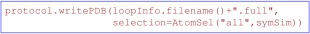
At the end of the calcOneStructure function introduced in Figure 3, add this call to write out the coordinates of all subunits with the suffix .full. symSim is the SymSimulation object created in Figure 8.
Ensemble Refinement
When a molecular system undergoes significant motion on timescales short relative to that of an experiment, the resulting observables will contain contributions from the various substates. A facility to fit an ensemble of structures to data was introduced73 and expanded significantly since the publication of Ref. 4. We now recommend sum averaging of energy terms over an ensemble to avoid implicit scaling of time so that the setup of an EnsembleSimulation object should now follow that in Figure 10. Most native Python terms which correspond to experimental observables have EnsembleSimulation support.
Figure 10.
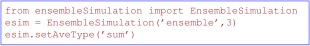
Code to create a three‐membered ensemble. Creation of the EnsembleSimulation makes copies of the current atom positions, velocities, and so forth. The constituent structures do not interact except by special ensemble‐aware energy terms. The sum averaging setting specifies that energies (including kinetic energy) increase in proportion to the ensemble size.
A major enhancement to the ensemble refinement facility has been the ability to determine ensemble member populations in concert with structure determination.53 Ensemble populations can be allowed to vary to improve fit, and to reduce the ensemble size required for a good fit. Ensemble populations are encoded in N‐sphere coordinates, x i:
| (4) |
| (5) |
| (6) |
⋮
| (7) |
| (8) |
with the radial component r taken to be 1, and the angular coordinates encoded as bond‐angles of pseudo atoms. Ensemble populations wi are then given as
| (9) |
and they obey the normalization condition . Because it is not useful to compute ensemble members with population zero, we further constrain the populations to lie in a reduced range by specifying to the minimum population we believe we can represent with a given set of data, so that
With this representation of ensemble populations, computation of the gradient with respect to pseudo atom coordinates is straightforward. Facilities within Xplor‐NIH are now provided to make it convenient to optimize ensemble populations for any ensemble energy term by providing the derivative with respect to ensemble population. As of this writing, ensemble population derivative support has been added to the SolnScatPot, SARDCPot, RDCCorrPot, CCRPot, and GyrPot terms. Support for additional terms can be added as needed.
In addition to setting a minimum ensemble population, instabilities due to wild gyrations in ensemble population values early in structure calculations are avoided by introducing a stabilizing energy term:
| (10) |
where is a force constant which is generally large at the start of a structure calculation, and small at the end. The target population values might initially take values of , but can be tuned from prior knowledge, or during the course of a structure calculation.
Finally, symmetry may dictate that there be relationships between ensemble populations. Consider a symmetric dimer in which each subunit takes two conformations X and Y, neither of which influences the dimerization interface. In this case, there will be three distinct states denoted XX, YY, and XY, the last of which would be indistinguishable from YX. In this case, if the populations of the two subunit conformations are wX and wY, the populations of the full dimer would be and , respectively. Xplor‐NIH now has a facility to derive the three dimer populations from the two subunit populations with a rather general mechanism for specifying constraints between populations. In vector notation one can write
| (11) |
where are base populations defined in Eq. (9) and A i, and contain coefficients which define w i populations of the system of interest in terms of the base populations. For the dimer example discussed above, A i = 0, for all i and the nonzero elements of the are:
| (12) |
where the 0, 1, 2 states correspond to the dimer XX, YY, and XY states, respectively. Figure 11 shows the creation of a pop object which contains a description of the three state symmetric dimer system described above.
Figure 11.
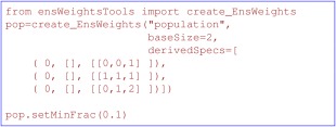
The pop object contains a description of the populations of a three‐state symmetric dimer with two substates in each subunit. The minimal population is set to be . The pop object is also an energy term, implementing the regularizing energy defined in Eq. (10).
Modern Data Formats
The NMR exchange format (NEF)74 is a standard simple file format intended to be used to store NMR data and derived restraints. As of this writing, it supports storing chemical shift data, peak lists from multidimensional NOE experiments, RDCs and distance and torsion angle restraints. Xplor‐NIH can read and write NEF files as shown in Figure 12.
Figure 12.
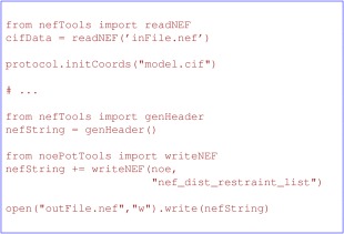
Examples of reading and writing NEF formatted files. The readNef function will generate PSF information, and additional energy terms can be initialized using content in the cifData object. Here, coordinates are read in mmCIF format. For writing a NEF file the genHeader function will generate connectivity information and the noePotTools.writeNEF will then add restraint data from noe, an NOEPot object defined previously in the script (not shown).
The mmCIF file format is a successor to the venerable PDB format which addresses limitations of the later including a rather limited number of possible chains and fixed precision atomic coordinates. The mmCIF format also allows one to define custom fields to represent per‐atom data. Xplor‐NIH supports reading and writing these files.
Other Xplor‐NIH Facilities
Probabilistic NOE assignment algorithm for automated structure determination (PASD)
Xplor‐NIH includes the PASD facility for automatic NOE assignment from completely automatically peak‐picked multi‐dimensional NMR spectra, with simultaneous structure determination.8 The key features of this facility are:
An initial analysis of possible assignments before structure determination, giving high‐likelihood to assignments which are consistent with other assignments.
For a given NOE peak, multiple possible assignments are simultaneously enabled.
A linear NOE potential is used in early stages of the calculation so that all assignments contribute equal magnitude forces.
Successive passes of assignment calculation are not based on previously determined structures, thus greatly reducing the chances of converging on incorrect structure/assignment combinations.
More details can be found in Refs. 8 and 75.
The PASD algorithm has been found to be highly robust in the face of bad NOE data (including missing or bad chemical shift assignments), with the ability to tolerate about 80% bad long‐range data (i.e., data between residues separated by more than five residues in primary sequence). Failure of the method is clearly indicated by lack of convergence of assignment likelihoods, and by a large spread (poor precision) in the calculated set of structures. The following input formats are currently supported: NEF, nmrdraw, nmrstar, pipp, and xeasy. It is a simple task to write filters to support additional formats.
The user interface to PASD is a set of Tcl scripts, examples of which can be found in the eginput/pasd/* subdirectories of the Xplor‐NIH distribution. These scripts are written at a very high level such that they are each to understand and modify.
Chirality determination in small molecules
Xplor‐NIH contains support for the progressive stereo locking (PSL) algorithm76 for determination of the chirality of natural products and other small molecules using primarily RDC data measured in aligning media coupled with NOE‐derived distance restraints. In this protocol, chirality at the centers in question are allowed to float during structure calculation by removing the associated improper dihedral term and greatly relaxing the force constants on the associated bond angle terms. It was found that the PSL approach results in a unique configuration (for rigid molecules) or a very small number of configurations (for less rigid molecules), and has been applied to systems with up to 14 chiral centers. Facilities developed for this algorithm include the protocol itself (available in the eginput/psl subdirectory of the Xplor‐NIH distribution) coupled with facilities for determination of absolute chirality in the chirality module.
Analysis and validation
Information on how well a given structure satisfies experimental restraints is given in the standard coordinate files produced by the StructureLoop class introduced in Figure 3. The resulting coordinate files contain a summary of the number of restraints which are violated by more than a given standard (but adjustable) threshold value, and the root‐mean‐square deviation of the difference between calculated and experimental observables. A detailed listing of the specific violations for each term is given in a separate file whose name has a .viols suffix. More global structural analysis is triggered by setting the genViolationStats argument to True, and is based on the top fraction of structures specified by averageTopFraction, after all structures have been sorted from low to high energy using the terms in averageSortPots. The results of the analysis are stored in a file with the .stats suffix, which reports on all the energy terms specified in averagePotList. The .stats file contains averages of fit RMSD and number of violations for each energy term. For some energy terms, averages of associated properties are reported in the .stats file. For instance, average alignment tensor properties and R‐factor fit metric are reported for the RDCPot term. For most terms for which the concept of violation is meaningful, a list of restraints violated most often is listed in the .stats file, along with the fraction of the analyzed set of structures for which the violation was present. A persistently violated restraint frequently indicates some sort of problem with the input data. The averagePotList argument is also used to compute a regularized average structure to which the analyzed structures are fit (using the selection string given in the argument averageFitSel) to report the coordinate precision. Although not exercised in Figure 3, the average structure can be written out by specifying the extra argument averageFilename to StructureLoop. Final validation of a structure can be accomplished using the wwPDB Validation Service.77 This performs the same validation procedure as used during submission of a structure to the PDB.
Helper programs
A number of helper programs are distributed with Xplor‐NIH so that common tasks can be performed from the Unix command line without writing or editing a separate script. These programs include
targetRMSD—rigid‐body fit of one or more structures to a target structure and compute the positional RMSD.
calcTensor—given RDC data and one or more structures, compute the alignment tensor via singular value decomposition, and report the fit of back‐calculated RDCs to the data. The back‐calculated RDCs can be output as text, or as a plot.
calcSARDC—given RDC data measured in steric alignment media and one or more structures, back‐calculate RDCs and report the fit to the data, optionally in graphical form.
calcDaRh—Calculate an estimate of the alignment tensor D a and rhombicity from input RDC values (without structures) using the assumption of isotropically distributed bond vectors and a maximum likelihood approach.78
calcSAXS—Given a molecular structure, compute a SAXS or SANS curve, optionally fitting to experiment.
torsionReport—Generate report on all protein torsion angle values for one or more PDB files.
aveStruct—given a set of input files, compute an unregularized average structure.
ens2pdb—Converts a set of structure files to a single PDB file, with structures separated by MODEL records resulting in a file for PDB submission.
contactMap—Generate contact map from one or more PDB files.
ramaStrip—Given one or more input PDB files, generate a sequence of two‐dimensional Ramachandran plots, one for each residue. In each plot is plotted the ϕ/ψ position associated with each input PDB, overlaid on contours indicating residue‐specific allowed regions as determined by the methodology described in Ref. 18.
scriptMaker—a graphical interface for generating Xplor‐NIH scripts.
A full list and documentation can be found here: https://nmr.cit.nih.gov/xplor-nih/doc/current/helperPrograms/.
Test suite
Xplor‐NIH is distributed with a full suite of regression tests both in the source and binary‐only packages. These tests are essential to obtain confidence that the package operates properly. For end‐users, possible problems can be caused by moving to a system with slightly different hardware or operating system configuration different from those used for compilation. For developers, a seemingly unrelated change might break some other functionality within Xplor‐NIH. These tests provide some assurance that the package does indeed behave as expected, and allows quick identification as to where an error is located. In the source package, components are tested hierarchically: the C++ template library contains a test suite, as does the IVM and each energy term. In both the source and binary distributions, the XPLOR, Python and Tcl interfaces contain a large collection of test scripts along with the expected output. The bin/testDist command invokes an automated procedure which runs each script and reports discrepancies. These tests are essential to validate a new installation of Xplor‐NIH.
Extensive sets of full scripts with all supporting data are present in the eginput subdirectory of a Xplor‐NIH distribution. Basic validation of the suite of example scripts in the eginput subdirectory is performed using the runAll script in that directory, while a more thorough validate script will run a complete calculation for one or more examples, and check that the computed results are within a tolerance of published values.
Conclusion
This article provides an overview of using the Xplor‐NIH Python interface for structure determination. The example code here is by necessity fragmentary and incomplete. Many facilities have not been touched upon at all. Much more complete documentation is available from the Xplor‐NIH website at https://nmr.cit.nih.gov/xplor-nih/doc/current/. Specific questions should be addressed to the Xplor‐NIH mailing list at xplor‐nih@nmr.cit.nih.gov. Proper journal citation for this program should include the original Ref. 1 and this article.
Acknowledgments
Many of the components of this package are the product of a large number of workers over three decades. The authors thank the many NMR groups who have given useful feedback over the years. The authors declare no conflicts of interest.
Footnotes
Of course, this facility can be used in non‐protein contexts. We use this word here for convenience.
References
- 1. Schwieters CD, Kuszewski JJ, Tjandra N, Clore GM (2003) The Xplor‐NIH NMR molecular structure determination package. J Magn Reson 160:65–73. [DOI] [PubMed] [Google Scholar]
- 2. Brünger AT (1993) XPLOR Manual Version 3.1. New Haven: Yale University Press. [Google Scholar]
- 3.Available at: http://www.swig.org/. [Google Scholar]
- 4. Schwieters CD, Kuszewski JJ, Clore GM (2006) Using Xplor‐NIH for NMR molecular structure determination. Progr NMR Spectrosc 48:47–62. [Google Scholar]
- 5. Lutz M, Ascher D (2004) Learning python, 2th ed. Sebastopol: O'Reilly. [Google Scholar]
- 6. Schwieters CD, Clore GM (2001) Internal coordinates for molecular dynamics and minimization in structure determination and refinement. J Magn Reson 152:288–302. [DOI] [PubMed] [Google Scholar]
- 7.Available at: http://nmr.cit.nih.gov/xplor-nih/doc/current/python/ref/index.html.
- 8. Kuszewski J, Schwieters CD, Garrett DS, Byrd RA, Tjandra N, Clore GM (2004) Completely automated, highly error tolerant macromolecular structure determination from multidimensional nuclear Overhauser enhancement spectra and chemical shift assignments. J Am Chem Soc 126:6258–6273. [DOI] [PubMed] [Google Scholar]
- 9.Available at: http://www.numpy.org/
- 10. Hunter JD (2007) Matplotlib: a 2D graphics environment. Comput Sci Eng 9:90–95. [Google Scholar]
- 11.Available at: http://www.pbspro.org/
- 12. Yoo A, Jette M, Grondona M (2003) SLURM: simple linux utility for resource management: job scheduling strategies for parallel processing, volume 2862 of lecture notes in computer science. Berlin, Heidelberg: Springer‐Verlag, pp 44–60. [Google Scholar]
- 13. Schwieters CD, Clore GM (2014) Using small angle solution scattering data in Xplor‐NIH structure calculations. Prog NMR Spectrosc 80:1–11. [DOI] [PMC free article] [PubMed] [Google Scholar]
- 14. Gong Z, Schwieters CD, Tang C (2015) Conjoined use of EM and NMR in RNA structure refinement. Plos One 10:e0120445. [DOI] [PMC free article] [PubMed] [Google Scholar]
- 15. Brünger AT, Kuriyan J, Karplus M (1987) Crystallographic R‐factor refinement by molecular‐dynamics. Science 235:458–460. [DOI] [PubMed] [Google Scholar]
- 16. Brünger AT, In Isaacs NW, Taylor MR, Eds. (1988) Crystallographic computing 4: techniques and new technologies. (IUCr Crystallographic Symposia No. 3.). Oxford: International Union of Crystallography and Oxford University Press; pp. 126–140. [Google Scholar]
- 17. Brünger AT (1992) Free R‐value—a novel statistical quantity for assessing the accuracy of crystal‐structures. Nature 355:472–475. [DOI] [PubMed] [Google Scholar]
- 18. Bermejo GA, Clore GM, Schwieters CD (2012) Smooth statistical torsion angle potential derived from a large conformational database via adaptive kernel density estimation improves the quality of NMR protein structures. Protein Sci 21:1824–1836. [DOI] [PMC free article] [PubMed] [Google Scholar]
- 19. Bermejo GA, Clore GM, Schwieters CD (2016) Improving NMR structures of RNA. Structure 24:806–815. [DOI] [PMC free article] [PubMed] [Google Scholar]
- 20. Nilges M (1993) A calculational strategy for the solution structure determination of symmetric dimers by 1H‐NMR. Proteins 17:297–309. [DOI] [PubMed] [Google Scholar]
- 21. Rieping W, Habeck M, Nilges M (2005) Modeling errors in NOE data with a lognormal distribution improves the quality of NMR structures. J Am Chem Soc 127:16026–16027. [DOI] [PubMed] [Google Scholar]
- 22. Cornilescu G, Bax A (2000) Measurement of proton, nitrogen, and carbonyl chemical shielding anisotropies in a protein dissolved in a dilute liquid crystalline phase. J Am Chem Soc 122:10143–10154. [Google Scholar]
- 23. Ryabov Y, Suh J‐Y, Grishaev A, Clore GM, Schwieters CD (2009) Using the experimentally determined components of the overall rotational diffusion tensor to restrain molecular shape and size in NMR structure determination of globular proteins and protein‐protein complexes. J Am Chem Soc 131:9522–9531. [DOI] [PMC free article] [PubMed] [Google Scholar]
- 24. Ryabov Y, Clore GM, Schwieters CD (2010) Direct use of 15N relaxation rates as experimental restraints on molecular shape and orientation for docking of protein‐protein complexes. J Am Chem Soc 132:5987–5989. [DOI] [PMC free article] [PubMed] [Google Scholar]
- 25. Ryabov Y, Schwieters CD, Clore GM (2011) Impact of 15N R2/R1 relaxation restraints on molecular size, shape and bond vector orientation for NMR protein structure determination with sparse distance restraints. J Am Chem Soc 133:6154–6157. [DOI] [PMC free article] [PubMed] [Google Scholar]
- 26. Fenwick R, Schwieters CD, Vögeli B (2016) Direct investigation of slow correlated dynamics in proteins via dipolar interactions. J Am Chem Soc 138:8412–8421. [DOI] [PMC free article] [PubMed] [Google Scholar]
- 27. Wang Y, Schwieters CD, Tjandra N (2012) Parameterization of solvent‐protein interaction and its use on NMR protein structure determination. J Magn Res 221:76–84. [DOI] [PMC free article] [PubMed] [Google Scholar]
- 28. Iwahara J, Schwieters CD, Clore GM (2004) Ensemble approach for NMR structure refinement against 1H paramagnetic relaxation enhancement data arising from a flexible paramagnetic group attached to a macromolecule. J Am Chem Soc 126:5879–5896. [DOI] [PubMed] [Google Scholar]
- 29. Tang C, Iwahara J, Clore GM (2006) Visualization of transient encounter complexes in protein‐protein association. Nature 444:383–386. [DOI] [PubMed] [Google Scholar]
- 30. Barfield M (2002) Structural dependencies of interresidue scalar coupling (h3)J(NC') and donor 1H chemical shifts in the hydrogen bonding regions of proteins. J Am Chem Soc 124:4158–4168. [DOI] [PubMed] [Google Scholar]
- 31. Sass HJ, Schmid FF, Grzesiek S (2007) Correlation of protein structure and dynamics to scalar couplings across hydrogen bonds. J Am Chem Soc 129:5898–5903. [DOI] [PubMed] [Google Scholar]
- 32. Clore GM, Nilges M, Sukumaran DK, Brünger AT, Karplus M, Gronenborn AM (1986) The three‐dimensional structure of α1‐purothionin in solution: combined use of nuclear magnetic resonance, distance geometry and restrained molecular dynamics. EMBO J 5:2729–2735. [DOI] [PMC free article] [PubMed] [Google Scholar]
- 33. Vuister GW, Delaglio F, Bax A (1993) The use of 1J coupling constants as a probe for protein backbone conformation. J Biomol NMR 3:67–80. [DOI] [PubMed] [Google Scholar]
- 34. Kuszewski J, Qin J, Gronenborn AM, Clore GM (1995) The impact of direct refinement against and chemical shifts on protein structure determination by NMR. J Magn Reson Series B 106:92–96. [DOI] [PubMed] [Google Scholar]
- 35. Spera S, Bax A (1991) Empirical correlation between protein backbone conformation and C and C 13C nuclear‐magnetic‐resonance chemical shifts. J Am Chem Soc 113:5490–5492. [Google Scholar]
- 36. Kuszewski J, Gronenborn AM, Clore GM (1995) The impact of direct refinement against proton chemical shifts in protein structure determination by NMR. J Magn Reson Series B 107:293–297. [DOI] [PubMed] [Google Scholar]
- 37. Kuszewski J, Gronenborn AM, Clore GM (1996) A potential involving multiple proton chemical shift restraints for non‐stereospecifically assigned methyl and methylene protons. J Magn Reson Series B 112:79–81. [DOI] [PubMed] [Google Scholar]
- 38. Yip P, Case DA (1989) A new method for refinement of macromolecular structures based on nuclear overhauser effect spectra. J Magn Reson 83:643–648. [Google Scholar]
- 39. Nilges M, Habazettl J, Brünger AT, Holak TA (1991) Relaxation matrix refinement of the solution structure of squash trypsin‐inhibitor. J Mol Biol 219:499–510. [DOI] [PubMed] [Google Scholar]
- 40. Tjandra N, Garrett DS, Gronenborn AM, Bax A, Clore GM (1997) Defining long range order in NMR structure determination from the dependence of heteronuclear relaxation times on rotational diffusion anisotropy. Nat Struct Biol 4:443–449. [DOI] [PubMed] [Google Scholar]
- 41. Clore GM, Gronenborn AM, Szabo A, Tjandra N (1998) Determining the magnitude of the fully asymmetric diffusion tensor from heteronuclear relaxation data in the absence of structural information. J Am Chem Soc 120:4889–4890. [Google Scholar]
- 42. Sass HJ, Musco G, Stahl SJ, Wingfield PT, Grzesiek S (2001) An easy way to include weak alignment constraints into NMR structure calculations. J Biomol NMR 21:275–280. [DOI] [PubMed] [Google Scholar]
- 43. Meiler J, Blomberg N, Nilges M, Griesinger C (2000) A new approach for applying residual dipolar couplings as restraints in structure elucidation. J Biomol NMR 16:245–252. [DOI] [PubMed] [Google Scholar]
- 44. Franks WT, Wylie BJ, Schmidt HL, Nieuwkoop AJ, Mayrhofer RM, Shah GJ, Graesser DT, Rienstra CM (2008) Dipole tensor‐based atomic‐resolution structure determination of a nanocrystalline protein by solid‐state NMR. Proc Natl Acad Sci USA 106:4621–4626. [DOI] [PMC free article] [PubMed] [Google Scholar]
- 45. Lipsitz RS, Sharma Y, Brooks BR, Tjandra N (2002) Hydrogen bonding in high‐resolution protein structures: a new method to assess NMR protein geometry. J Am Chem Soc 124:10621–10626. [DOI] [PubMed] [Google Scholar]
- 46. Grishaev A, Bax A (2004) An empirical backbone‐backbone potential in proteins and its application to NMR structure refinement and validation. J Am Chem Soc 126:7281–7292. [DOI] [PubMed] [Google Scholar]
- 47. Kuszewski J, Schwieters CD, Clore GM (2001) Improving the accuracy of NMR structures of DNA by means of a database potential of mean force describing base‐base positional interactions. J Am Chem Soc 123:3903–3918. [DOI] [PubMed] [Google Scholar]
- 48. Clore GM, Kuszewski J (2003) Improving the accuracy of NMR structures of RNA by means of conformational database potentials of mean force as assessed by complete dipolar coupling cross‐validation. J Am Chem Soc 125:1518–1525. [DOI] [PubMed] [Google Scholar]
- 49. Zuo X, Tiede DM (2005) Resolving conflicting crystallographic and NMR models for solution‐state DNA with solution X‐ray diffraction. J Am Chem Soc 127:16–17. [DOI] [PubMed] [Google Scholar]
- 50. Schwieters CD, Clore GM (2008) A pseudopotential for improving the packing of ellipsoidal protein structures determined by NMR. J Phys Chem B 112:6070–6073. [DOI] [PubMed] [Google Scholar]
- 51. Kuszewski J, Gronenborn AM, Clore GM (1999) Improving the packing and accuracy of NMR structures with a pseudopotential for the radius of gyration. J Am Chem Soc 121:2337–2338. [Google Scholar]
- 52. Huang J‐R, Grzesiek S (2010) Ensemble calculations of unstructured proteins constrained by RDC and PRE data: a case study of urea‐denatured ubiquitin. J Am Chem Soc 132:694–705. [DOI] [PubMed] [Google Scholar]
- 53. Deshmukh L, Schwieters CD, Grishaev A, Ghirlando R, Baber JL, Clore GM (2013) Structure and dynamics of full‐length HIV‐1 capsid protein in solution. J Am Chem Soc 135:16133–16147. [DOI] [PMC free article] [PubMed] [Google Scholar]
- 54. Camilloni C, Vendruscolo M (2015) A tensor‐free method for the structural and dynamical refinement of proteins using residual dipolar couplings. J Phys Chem B 9:653–661. [DOI] [PubMed] [Google Scholar]
- 55. Straus SK, Scott WRP, Schwieters CD, Marvin DA (2011) Consensus structure of Pf1 filamentous bacteriophage from X‐ray fibre diffraction and solid‐state NMR. Eur Biophys J 40:221–234. [DOI] [PMC free article] [PubMed] [Google Scholar]
- 56. Engh RA, Huber R (1991) Accurate bond and angle parameters for X‐ray protein structure refinement. Acta Cryst A47:392–400. [Google Scholar]
- 57. Parkinson G, Vojtechovsky J, Clowney L, Brünger AT, Berman HM (1996) New parameters for the refinement of nucleic acid‐containing structures. Acta Crystallogr D Biol Crystallogr 52:57–64. [DOI] [PubMed] [Google Scholar]
- 58. Kuszewski J, Gronenborn AM, Clore GM (1996) Improving the quality of NMR and crystallographic protein structures by means of a conformational database potential derived from structure databases. Protein Sci 5:1067–1080. [DOI] [PMC free article] [PubMed] [Google Scholar]
- 59. Kuszewski J, Gronenborn AM, Clore GM (1997) Improvements and extensions in the conformational database potential for the refinement of NMR and X‐ray structures of proteins and nucleic acids. J Magn Reson 125:171–177. [DOI] [PubMed] [Google Scholar]
- 60. Nilges M, Clore GM, Gronenborn AM (1988) Determination of three‐dimensional structures of proteins from interproton distance data by hybrid distance geometry‐dynamical simulated annealing calculations. FEBS Lett 229:317–324. [DOI] [PubMed] [Google Scholar]
- 61. Nabuurs SB, Nederveen AJ, Vranken W, Doreleijers JF, Bonvin AMJJ, Vuister GW, Vriend G, Spronk CAEM (2004) DRESS: a database of refined solution NMR structures. Proteins 55:483–486. [DOI] [PubMed] [Google Scholar]
- 62. Lazaridis T, Karplus M (1999) Effective energy function for proteins in solution. Proteins 35:133–152. [DOI] [PubMed] [Google Scholar]
- 63. Tian Y, Schwieters CD, Opella SJ, Marassi FM (2014) A practical implicit solvent potential for NMR structure calculation. J Magn Res 243:54–64. [DOI] [PMC free article] [PubMed] [Google Scholar]
- 64. Tian Y, Schwieters CD, Opella SJ, Marassi FM (2015) A practical implicit membrane potential for NMR structure calculations of membrane proteins. Biophys J 109:574–585. [DOI] [PMC free article] [PubMed] [Google Scholar]
- 65. Tian Y, Schwieters CD, Opella SJ, Marassi FM (2017) High quality NMR structures: a new force field with implicit water and membrane solvation for Xplor‐NIH. J Biomol NMR 67:35–49. [DOI] [PMC free article] [PubMed] [Google Scholar]
- 66. Nederveen AJ, Doreleijers JF, Vranken W, Miller Z, Spronk CAEM, Nabuurs SB, Guentert P, Livny M, Markley JL, Nilges M, Ulrich EL, Kaptein R, Bonvin AMJJ (2005) "RECOORD: a recalculated coordinates database of 500+ proteins from the PDB using restraints from the BioMagResBank. Proteins 59:662–672. [DOI] [PubMed] [Google Scholar]
- 67. Jorgensen WL, Tirado‐Rives J (1988) The OPLS potential functions for proteins—energy minimizations for crystals of cyclic‐peptides and crambin. J Am Chem Soc 110:1666–1671. [DOI] [PubMed] [Google Scholar]
- 68. Weiner SJ, Kollman PA, Case DA, Singh UC, Ghio C, Alagona G, Profeta S, Weiner P (1984) A new force‐field for molecular mechanical simulation of nucleic‐acids and proteins. J Am Chem Soc 106:765–784. [Google Scholar]
- 69. Schuettelkopf AW, van Aalten DMF (2004) PRODRG—a tool for high‐throughput crystallography of protein‐ligand complexes. Acta Crystallograph D60:1355–1363. [DOI] [PubMed] [Google Scholar]
- 70. Kleywegt GJ, Zou JY, Kjeldgaard M, Jones TA, In: Rossmann MG, Arnold E, Eds. (2001) International Tables for Crystallography Volume F: Crystallography of biological macromolecules. Dordrecht: Kluwer Academic Publishers; pp. 353–356, 366–367. [Google Scholar]
- 71.Available at: http://webapps.ccpn.ac.uk/acpype/
- 72. Bardiaux B, van Rossum BJ, Nilges M, Oschkinat H (2012) Efficient modeling of symmetric protein aggregates from NMR data. Angew Chem Int Ed Engl 51:6916–6919. [DOI] [PubMed] [Google Scholar]
- 73. Clore GM, Schwieters CD (2004) How much backbone motion in ubiquitin is required to be consistent with dipolar coupling data measured in multiple alignment media as assessed by independent cross‐validation. J Am Chem Soc 126:2923–2938. [DOI] [PubMed] [Google Scholar]
- 74. Gutmanas A, Adams P, Berman H, Case D, Fogh R, Hendrickx P, Herrmann T, Kleywegt G, Kobayashi N, Lange O, Markley J, Montelione G, Nilges M, Ragan T, Schwieters C, Tejero R, Ulrich E, Velankar S, Vranken W, Wishart D, Westbrook J, Bardiaux B, Güntert P, Wedell J (2015) NMR exchange format: a unified and open standard for representation of NMR restraint data. Nat Struct Bio 22:433–434. [DOI] [PMC free article] [PubMed] [Google Scholar]
- 75. Kuszewski JJ, Augustine Thottungal R, Clore GM, Schwieters CD (2008) Automated error‐tolerant macromolecular structure determination from multidimensional nuclear Overhauser enhancement spectra and chemical shift assignments: improved robustness and performance of the PASD algorithm. J Biomol NMR 41:221–239. [DOI] [PMC free article] [PubMed] [Google Scholar]
- 76. Cornilescu G, Ramos Alvarenga RF, Wyche TP, Bugni TS, Gil RR, Cornilescu CC, Westler WM, Markley JL, Schwieters CD (2017) Progressive stereo locking (PSL): a residual dipolar coupling based force field method for determining the relative configuration of natural products and other small molecules. ACS Chem Biol. 7:2157–2163. [DOI] [PMC free article] [PubMed] [Google Scholar]
- 77.Available at: https://validate-rcsb-1.wwpdb.org/
- 78. Warren JJ, Moore PB (2001) A maximum likelihood method for determining and R for sets of dipolar coupling data. J Magn Res 149:271–275. [DOI] [PubMed] [Google Scholar]