

Abstract
Purpose
To investigate deep reinforcement learning (DRL) based on historical treatment plans for developing automated radiation adaptation protocols for nonsmall cell lung cancer (NSCLC) patients that aim to maximize tumor local control at reduced rates of radiation pneumonitis grade 2 (RP2).
Methods
In a retrospective population of 114 NSCLC patients who received radiotherapy, a three‐component neural networks framework was developed for deep reinforcement learning (DRL) of dose fractionation adaptation. Large‐scale patient characteristics included clinical, genetic, and imaging radiomics features in addition to tumor and lung dosimetric variables. First, a generative adversarial network (GAN) was employed to learn patient population characteristics necessary for DRL training from a relatively limited sample size. Second, a radiotherapy artificial environment (RAE) was reconstructed by a deep neural network (DNN) utilizing both original and synthetic data (by GAN) to estimate the transition probabilities for adaptation of personalized radiotherapy patients’ treatment courses. Third, a deep Q‐network (DQN) was applied to the RAE for choosing the optimal dose in a response‐adapted treatment setting. This multicomponent reinforcement learning approach was benchmarked against real clinical decisions that were applied in an adaptive dose escalation clinical protocol. In which, 34 patients were treated based on avid PET signal in the tumor and constrained by a 17.2% normal tissue complication probability (NTCP) limit for RP2. The uncomplicated cure probability (P+) was used as a baseline reward function in the DRL.
Results
Taking our adaptive dose escalation protocol as a blueprint for the proposed DRL (GAN + RAE + DQN) architecture, we obtained an automated dose adaptation estimate for use at ∼2/3 of the way into the radiotherapy treatment course. By letting the DQN component freely control the estimated adaptive dose per fraction (ranging from 1–5 Gy), the DRL automatically favored dose escalation/de‐escalation between 1.5 and 3.8 Gy, a range similar to that used in the clinical protocol. The same DQN yielded two patterns of dose escalation for the 34 test patients, but with different reward variants. First, using the baseline P+ reward function, individual adaptive fraction doses of the DQN had similar tendencies to the clinical data with an RMSE = 0.76 Gy; but adaptations suggested by the DQN were generally lower in magnitude (less aggressive). Second, by adjusting the P+ reward function with higher emphasis on mitigating local failure, better matching of doses between the DQN and the clinical protocol was achieved with an RMSE = 0.5 Gy. Moreover, the decisions selected by the DQN seemed to have better concordance with patients eventual outcomes. In comparison, the traditional temporal difference (TD) algorithm for reinforcement learning yielded an RMSE = 3.3 Gy due to numerical instabilities and lack of sufficient learning.
Conclusion
We demonstrated that automated dose adaptation by DRL is a feasible and a promising approach for achieving similar results to those chosen by clinicians. The process may require customization of the reward function if individual cases were to be considered. However, development of this framework into a fully credible autonomous system for clinical decision support would require further validation on larger multi‐institutional datasets.
Keywords: adaptive radiotherapy, deep learning, lung cancer, reinforcement learning
1. Introduction
Most nonsmall cell lung cancer (NSCLC) patients are inoperable due to locally advanced disease or distant metastases and thus radiation therapy (radiotherapy) becomes the main option for treatment of these patients. However, treatment outcomes remain relatively poor despite significant advances in the technologies of radiotherapy planning, image‐guidance, and delivery.1 It is conjectured that escalation of radiation dose is an option to improve treatment outcome results. For instance, a dose increment by 1 Gy can lead to 1% improvement in local progression free survival.2, 3 However, this has not always been demonstrated to be the case, as was learned from RTOG‐0617 clinical trial results, where dose escalation has led to surprisingly negative results.4 Though the specific causes of this negative finding are still being worked out, it is clear that dose escalation cannot be employed using a one‐size‐fits‐all approach to the patient population. While necessary for cancer treatment, radiotherapy provides cure but can also pose risks that need to be tailored according to each individual patients characteristics. For treatment of lung cancer, a major limiting constraint to dose escalation is the toxicity risk from thoracic irradiation that leads to radiation‐induced pneumonitis (RP). RP causes cough, fever, etc, and it affects the quality of life for patients even if the local control (LC) of the tumor is assured. Therefore, an important question that the current studies are attempting to address is: can machine learning algorithms identify from patient characteristics an optimal dose schedule to render LC with maximally reduced RP in an individual patient? However, before attempting to address this challenging question, we need to demonstrate that machine learning algorithms can actually be taught to mimic clinicians decision making processes.
With the latest advances in machine reinforcement learning (RL) algorithms, which provide better dynamic learning options, we are poised to explore the feasibility of automated decision making for dose escalation in NSCLC patients. Traditional machine learning methods have witnessed increased applications in radiotherapy including quality assurance, computer‐aided detection, image‐guided radiotherapy, respiratory motion management, and now outcomes prediction.5 However, traditional machine learning methods may lack the ability to handle the dynamics of highly complex decision‐making process in a clinical radiotherapy environment. For instance, our institutional protocol UMCC 2007‐1232, 3 defines dose escalation under a sophisticated adaptation policy (see Section 2.G.2) towards improved treatment outcomes. Thus, it could be utilized as a suitable testbed to assess our proposed RL methods for automated radiation adaptation. The rationale for utilizing reinforcement learning in automating radiation dose adaptation is that it allows exploration of all possible paths into the future so that expected benefits and risks can be weighed into the decision‐making process. In an analogous fashion such as playing chess or board games, the decision maker needs to explore the consequences of the next moves and develop an optimal strategy to win the game, which in our case is controlling cancer while reducing treatment side effects. To realize this task within the complex radiotherapy environment, we developed dynamical procedures to utilize the existing historical treatment plans to represent the radiotherapy environment (Section 2.G.2), where the states within this environment are defined as predictor factors of local control (LC) and radiation‐induced pneumonitis (RP) responses.
In recent years, deep learning applications have gained success in variety of fields including video games, computer vision, and pattern recognition. A key factor in this success is that deep learning can abstract and extract high‐level features directly from the data. This helps avoid complex feature engineering or delicate feature hand‐crafting and selection for an individual task.6 Recent studies have demonstrated that using a class of deep learning algorithms based on convolution neural networks can efficiently replace traditional feature selection in image segmentation. while at the same time providing superior performance.7, 8 These strengths motivated Google DeepMind's incorporation of deep neural networks (DNN) into the known Q‐learning search algorithm of RL,9 which enabled it to master a diverse range of Atari games with human‐level performance using the raw pixels and scores as inputs.10 The DQN algorithm has been shown to display actions similar to human instincts in playing these games. Such ability was demonstrated by AlphaGo when it dethroned the world champion of the ancient Chinese game GO, a 19 × 19 grid board game considered to have intractable (316! ≃ 10678) possibilities. The sheer complexity of GO renders the ability to make human decisions from intuitive intelligence indispensable for playing properly and having a credible chance at winning. This study tends to pursue the characteristic of intuition‐driven decisions in the DQN for mimicking and comparing clinicians dose adaptation decisions in treatment planning. However, there are millions of records with detailed moves of previously played games that could be used in training the DQN algorithm; this is a luxury that we do not possess in the clinical or the radiotherapy world. Therefore, we also incorporated new developments in deep learning for generating synthetic data to help meet the goal of training automated actions owing to the demand of high‐sample‐size requirement by the DQN. Specifically, we deployed three different DNNs to tackle several problems in building a machine learning approach for completing automation of clinical decision‐making for adaptive radiotherapy, see Fig. 1(b). The first DNN (GAN, Section 2.E) aims to generate sufficiently large patient data from existing small‐sized observations for training the simulated radiotherapy environment. The second DNN is tasked to learn the radiotherapy environment, i.e., where and how states would transit under different actions (dose fraction modifications) based on the data synthesized from the GAN and real clinical data available, Section 2.G.3. The third DNN is the innovative DQN itself responsible for prompt and accurate evaluation of the different possible strategies (dose escalation/de‐escalation) and optimizing future rewards (radiotherapy outcomes). In contrast, classical RL methods such as the model‐free temporal difference (TD) algorithm,9 which require a sufficiently larger number of observations to be sampled and high consistency in the states (variables) and actions (decisions), do not fit well with the complex, real clinical radiotherapy environment where the data are noisy and complete information may be missing as well as limited sample size. Moreover, clinical decisions are in general likely to be more subjective than objective. These are some of the hurdles that our approach based on the three‐component DNN design attempts to overcome. We believe that the proper integration of these three components based on deep learning is essential for building a robust RL environment for decision support in radiotherapy adaptation.
Figure 1.

A three‐component DNN solution to overcome limited sample size and model the radiotherapy environment for DRL decision‐making.
In previous work,11 Kim et al. developed a Markov decision process (MDP) from the perspective of analytical radiobiological response to compute optimal fractionation schemes in radiotherapy. The MDP design was based on delicate assumptions on the latent behavior of the tumor and the organs‐at‐risk (OAR) with respect to given dose. Several numerical simulations were presented and their behavior, based on the assumptions made, were discussed but no realistic clinical scenarios were evaluated. Another similar approach based on analyzing stochastic processes of reinforcement learning with TD techniques12 was used to dynamically explore the transition probability with varying fractionation schedules. Based on simplified radiobiological assumptions, different reward (utility) functions were tested in preclinical cell culture data to nonuniformally optimize the prescribed dose per fraction.12
Here, implementation details and network architectures are described and organized as follows. In Section 2, we succinctly introduce the methods and rationale of our utilization; Section 3 demonstrates the results of the different components of our proposed approach and their benchmarking against real clinical protocol results. In Sections 4 and 5, we summarize our methods presentation as an integrated system and discuss future potential developments as well as the limitations of our current study.
2. Materials and methods
2.A. Overview
In our investigation to apply DQN for escalation of dose in NSCLC data, we first faced the obstacle of the absence of a well‐characterized radiotherapy environment (i.e., the rules of the game) as shown in Figs. 1(a) and 4. This is unlike the case of applying DQN to board games where complete information of the game rules are defined beforehand and also one can play the game repeatedly almost at no real cost. In the case of patient care in general or radiotherapy specifically, this would be ethically and practically prohibitive due to the consideration of patients’ safety and the cost of time. To alleviate this difficulty, we developed a radiotherapy artificial environment (RAE), also referred to as the (approximate) transition DNN in Section 2.G.3 for simulating the radiotherapy treatment response environment. Due to the limited available sample size, we combined the GAN with the transition DNN to support the fidelity of reconstructing a RAE. As the GAN can generate synthetic patient data very similar in its characteristics to the real ones, we then trained the RAE with mixed data; the synthesized data by the GAN and the available real clinical data. After the reconstruction of the radiotherapy environment, we introduced the DQN agent (decision maker) into this environment to interact with it, as indicated in Fig. 1(b) and evaluated its performance by learning the adaptive behavior of a dose escalation clinical protocol conducted successfully in our institution and recently published in JAMA Oncology.3
2.B. Datasets
We used historical treatment plans of 114 NSCLC patients for training our three‐component DRL for decision support of response‐based dose adaptation. The patients had been treated on prospective protocols under IRB approval as described in Ref. 13 All tumor and lung dose values were converted into their 2 Gy equivalents (EQD2) by an in‐house developed software using the linear‐quadric model with an α/β of 10 Gy and 4 Gy for the tumor and the lung, respectively. Generalized equivalent uniform doses (gEUDs) with various parameters a were calculated for gross tumor volumes (GTVs) and uninvolved lungs (lung volumes exclusive of GTVs). Blood samples were obtained at baseline and after approximately 1/3 and 2/3 of the scheduled radiation doses were completed. A total of 250 features including dosimetric variables, clinical factors, circulating microRNAs, single‐nucleotide polymorphisms (SNPs), circulating cytokines, and positron emission tomography (PET) imaging radiomics features before and during radiotherapy were collected. Pretreatment blood samples were analyzed for cytokine levels, micro RNAs (miRNAs), and single nucleotide polymorphisms (SNPs), which have been identified as candidates from the literature as related to lung cancer response. FDG‐PET/CT images were acquired using clinical protocols and the pretreatment and intratreatment PET images were registered to the treatment planning CT using rigid registration. The image features analysis was performed using customized routines in MATLAB and the features included metabolic tumor volume, intensity statistics, and texture‐derived metrics.14, 15 Part of this population, with dose adaptations at ∼2/3 of the way through treatment as served by Protocol UMCC 2007‐123,2, 3 are described in Section 2.G.1. Nine predictive features, defined in Eq. (14) with characteristics described in Table 1, were selected for modeling the RAE. These features are related to LC and RP2 responses based on Markov blankets and Bayesian analyses as detailed in Ref. 13 and briefly reviewed below.
Table 1.
Selected predictors for LC and RP2 and their characteristics
| Predictors | Biological/clinical characteristics | References |
|---|---|---|
| IL4 | Th2 cytokines. Regulates antibody production, haematopoiesis, and inflammation. Promotes the differentiation of naive helper T cells into Th2 cells. Decreases the production of Th1 cells | 26, 27, 28 |
| IL15 | Th1 cytokines. Induces activation and cytotoxicity of natural kill (NK) cells. Activates macrophages. Promotes proliferation and survival of T and B‐lymphocytes and NK cells | 26, 27, 28 |
| GLSZM.GLN | The gray‐level nonuniformity (GLN) feature of a gray‐level size zone matrix (GLSZM), defined by | Notations see Ref. 29 |
| GLRLM.RLN | The run‐length nonuniformity (RLN) feature of a gray‐level run length matrix (GLRLM) defined by | Notations see Ref. 29 |
| MCP1 | Chemokine expressed and secreted by adipocytes. Adipocyte expression of MCP‐1 is increased by TNF‐α | 30, 31 |
| TGFβ1 | Th2 cytokines. An important role in regulation of immune system. Produced by every leukocyte lineage, including lymphocytes, macrophages, and dendritic cells | 32 |
| Lung/tumor gEUD (α/β=4Gy,10Gy resp) | Generalized equivalent uniform dose of lung/tumor converted from EQD2 dose distributions: | 33, 34 |
| MTV | Metabolic tumor volume from PET imaging | – |
2.C. Variable selection for simulating radiotherapy environment
In order to define the radiotherapy environment via a large‐scale variable list, we used techniques based on Bayesian network graph theory, which allows for identifying the hierarchical relationships among the variables and outcomes of interest. The approach we used is based on identifying separate extended Markov blankets (MBs) for LC and RP2 from the above high‐dimensional dataset of 297 candidate variables. An MB of LC (or RP2) is the smallest set containing all variables carrying information about LC (or RP2) that cannot be obtained from any other variable (inner family); then for each member in the blanket of LC (or RP2), a next‐of‐kin MB for this member was also derived using a structure learning optimization algorithm.13 The algorithm combines efficient graph‐search techniques with statistical resampling for robust variable selection.13 The selected variables by this approach are summarized in Eq. (14). It should be emphasized that the purpose of this step is to provide an approximate radiotherapy environment that would allow simulating transitions between its states when the DQN agent is making decisions.
2.D. Deep neural networks
We mainly utilized deep neural networks (DNNs) for our proposed DRL approach and the main notations used are summarized here for convenience. Denoting data {x i } with labels {y i } such that , a DNN finds a function to weave through the data such that f DNN(x i ) ≅ y i as much as possible via the utility of three distinct components: neurons , layers of k neurons z = (z 1,…,z k ), and activation functions σ, see Fig. 6 (left). If a DNN has layers j = 0,…,ℓ, each of which has neurons, then j = 0 and ℓ would denote the first (input) and final (output) layer, respectively. An activation function connecting the neurons of the (j−1)th layer and those of the jth layer would satisfy:
| (1) |
where and represent the unknown weights and biases to be estimated. A typical choice of σ is a sigmoid or a rectified linear unit (ReLU), where we empirically choose σ = eLU 16 in this study for better convergence. Our best parameters are then derived from the forward dynamics and backward (error) propagation resulting from the DNN loss function:17
| (2) |
where are the Lagrange multipliers at layer j − 1 to preserve layerwise information Eq. (1).
Figure 6.

Random dropout DNNs (left) are used with data (z (0),z (l)) = (x,y) following notations in Sec. IID to reconstruct the transition probability of the environment (right), where is an approximation to the real world. Different layers are consequences of different actions made on the state (x 1,x 2,…,x 9). At each layer, 100 possible status of a patient are considered according to top transition probabilities. This process repeats itself at every state of each layer. [Color figure can be viewed at wileyonlinelibrary.com]
In this study, we primarily rely on the universality of DNNs to model the dynamic complexity hidden in the radiotherapy data. This universality refers to the capability of a neural network to approximate any continuous function (on a compact subset of ) with suitable activation functions.18 Due to limited patient sample size, we implemented random dropouts on neurons to efficiently mitigate overfitting19 throughout. In such scenario, randomly selected neurons are assigned zero weights, which is a form of regularization to prevent the network from overadaptation (overfitting) to the data during training process.
2.E. Generative adversarial nets
To alleviate the problem of small sample size in clinical datasets when modeling the complex state transitions in a radiotherapy environment, we utilize generative adversarial nets (GANs)20 to synthesize more radiotherapy patient‐like data. A GAN consists of two neural nets, one of which is generative (G) and responsible for generating synthetic data, and the other one is discriminative (D), which tries to measure the (dis)‐similarity between the synthesized and real data as shown in Fig. 2. The basic underlying idea is simple: by learning to confuse D, G can get more sophisticated in generating similar data through the following setup.
Figure 2.

GAN is used to generate new data, where G asks D to verify the authenticity of the data source. From latent points z, generated patients are synthesized as in G. With mixing with real and the generated patient data, D is trying to verify its source. [Color figure can be viewed at wileyonlinelibrary.com]
Denote the space containing the (original) dataset with distribution x ∼ P data, and there is a latent space with a prior distribution z ∼ P prior, where in our case a Gaussian distribution is assumed. The generative network tries to learn a map from to such that an induced probability distribution on is close to the original P data. The discriminative network then simultaneously learns to discriminate observations from the true data and the synthesized data generated by G. In general, G aims at generating indistinguishable data to confuse D, whereas D attempts to distinguish the data produced by G or not. They interact with each other in a competitive sense, hence the name GAN. The adversarial characters of D and G are created via the loss function of two‐player mini‐max game:
| (3) |
where .
Subsequently, we introduce the algorithm for generating synthetic data for building our DRL for dose adaption.
2.F. Deep Q‐networks
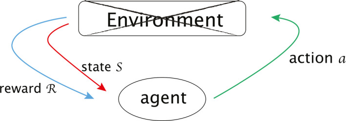
We are applying reinforcement learning to mimic how physicians decide dynamically on the dose fraction trade‐offs needed to prescribe to a certain patient. In reinforcement learning, there is the environment (an MDP) and an agent (an optimal action search algorithm). An agent takes charge of delivering actions in an environment, which is a world described by the various states s ∈ S in the environment. Upon a decision made under a current state , an agent receives corresponding reward R and gets promoted to another state. The transition between states and rewards R are feedback for the agent to perceive how to optimize its subsequent strategy for future actions. In our setting, an artificial agent would provide a second opinion or take place of a physician to deliver actions. Specifically, in this study, we will evaluate the required dose per fraction (adaptation) in the second period of a dose‐escalation radiotherapy treatment course. This agent will then interact with the radiotherapy artificial environment (RAE) reconstructed by the transitional DNN, Fig. 1(b), and adjust its own adaptation strategy based on received feedback.
Reinforcement learning is essentially formulated as a Markov decision process (MDP), denoted by , where be the space of states, is the collection of actions, is the reward function, and is the transition probability function between two states under an action with Ω a σ‐algebra of that naturally induces a conditional probability on space of next states t ∈ S from previous observation . A sequence of actions acting on an initial state leads to the dynamics of an MDP:
The Q‐learning search algorithm is a common method to find an optimal policy given an MDP or an RAE in our case, where a Q‐function is defined as the average discounted sum of rewards R in all future steps from current state s under a policy as in Eq. (4). The expectation value is considered in the sense of computing all possible paths starting from current states to represent all possible benefits received in the future. A discounting factor 0 ≤ γ ≤ 1 diminishes how we perceive future profits, providing a trade‐off between the importance of immediate reward versus future ones, i.e., short‐term responses versus long‐term outcomes.
In Q‐learning, an optimal policy is defined such that is satisfied when the value iteration scheme is adapted for computation. Via the Bellman's equation of off‐policy, the estimation of optimal is converted into an iterative sequence defined by9:
| (4) |
| (5) |
Upon the contraction mapping theorem,21 the convergence is reached at the unique fixed point as i→∞,
| (6) |
It can be noticed that computation of Eq. (5) can quickly become cumbersome when the cardinality |S| or is large. A recent solution proposed by Google DeepMind in Refs. 22 and 9 was to evaluate the Q‐function efficiently using supervised learning by DNNs by , where denotes the weights of DNNs in Eq. (1) at ith iteration with a sequence of loss functions to be minimized where:
| (7) |
where ρ is the probability distribution over policy sequences s and actions a also called the behaviour distribution. The loss function (7) can be understood to pursue a DNN sequence such that since (7) indicates:
| (8) |
by defining using at previous time t − 1. It is also understood that since one is not able to duplicate Y i exactly using a DNN approximator at every iteration i due to the finite degrees of freedom in DNN, namely (1), there always exists a small error to be compensated by the loss function (8), where Fig. 3 (left) shows their intertwined relationship. The sequence approached by both operations of the DNN and the loss function (8) can be proven to approximate the self‐iterated sequence , whose convergence to the optimal Q‐function is already guaranteed by the contraction mapping theorem. Summing up all the facts one derives an operational sequence by DNN as illustrated in Fig. 3 (right).
Figure 3.
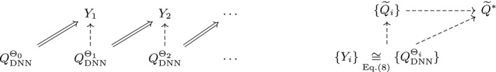
Machinery of DQN convergence. The left figure depicts the relation between {Y i } and , where arrow “⇒” denotes “create” and “” denotes “approximate”. The right figure illustrates the convergence relationship between three sequences.
The reason a DNN approximator fails to play the role directly is because of the finite approximation ability as mentioned above. Should a DNN have a perfect deformation such that is true for all i, then , which leads to the whole sequence by definition of (5). In this perfect case, the three characters , , and coincide. Due to the imperfect nature of the DNN approximator, the sequences , , and split with tiny differences from one another. In fact, the approximation accuracy of can impact the performance of a RL algorithm. A linear function approximator was first considered in early literature23 for computational reasons.
Besides using DNN for Q‐function iteration, DQN also utilizes techniques of experience replay memory and separating target networks to enhance its performance stability.22 As mentioned in Section 2.A, since our DQN agent is not allowed to explore optimal actions based on trial‐and‐error (risky actions) in real patients, our approach towards deep RL has to be different from common RL realizations used in nonclinical applications. The autonomous actions will instead be based on supervised learning from historical data rather than direct online (or model‐free) MDP learning as shown in Fig. 4, which could complement previously learned actions.
Figure 4.
An incomplete MDP where the environment is unknown or missing. [Color figure can be viewed at wileyonlinelibrary.com]
First, we attempt to reconstruct the environment of radiotherapy lung cancer patients from the existing data by an approximate transition of the real world. An accurate reconstruction of the environment will require a large amount of data to be available and reliable. This is why we utilized GAN to synthesize patient‐like data. After the reconstruction of the radiotherapy artificial environment (RAE), we then adopt deep Q‐learning to search for the optimal policy sequence for response‐based dose adaptation.
2.G. Deep reinforcement learning for radiotherapy dose adaptation
Before attempting to apply DRL for autonomous clinical decision‐making, a main purpose of this study was to evaluate whether we can actually utilize reinforcement learning to reproduce or mimic known clinical decisions that have been previously made. To achieve this goal, we design the following setup for dose adaptation of NSCLC patients and test its performance using data from a successful dose escalation protocol UMCC 2007‐123.2, 3 We will first provide a brief description of this dose escalation protocol, which will be used for benchmarking, followed by the design of our proposed DRL system to mimic this protocol.
2.G.1. Setting of protocol UMCC 2007‐123
Protocol UMCC 2007‐123 is a phase II dose escalation clinical trial.3 The study aimed to demonstrate that adaptive radiotherapy‐escalated radiation dose to the 18F‐fludeoxyglucose (FDG)‐avid region detected by midtreatment PET can improve local tumor control at 2 yr follow‐up, with a reasonable rate of radiotherapy‐induced toxicity. In a population of 42 patients who had inoperable or unresectable stage II to stage III NSCLC, the trial demonstrated an 82% local control. The radiation was delivered in 30 daily fractions of 2.1 to 5.0 Gy: 2.1 to 2.85 Gy fractions for the initial dose of approximately 50 Gy EQD2, and 2.85 to 5.0 Gy for the adaptive phase of treatments up to a total RT dose of 92 Gy EQD2.3 For the purpose of the DRL analysis, we present the protocol succinctly as follows. A treatment has total fractions f(t) and dose/fraction a(t) as functions of time t with:
| (9) |
where t * is the time for adaptation, T is the time of a complete treatment with 0<t *<T and are constants subject to the conditions Gy, Gy, and the total dose
| (10) |
As mentioned above, the first 50 Gy (EQD2) of radiation will be given based on pre‐PET and pre‐CT, the remaining dose is delivered to the target based on avid mid‐treatment FDG‐PET uptake as identified by the metabolic tumor volume (MTV). The protocol requires NTCP of lung to be maintained ≤ 17.2% (approximately equivalent to 20 Gy mean lung dose) based on estimates by the LKB model:24
| (11) |
with
| (12) |
The clinical endpoint for lung NTCP in the protocol UMCC 2007‐123 was RP2. The dataset of NSCLC has:
| (13) |
as shown in Fig. 5. We designed our agent to adapt dose after week 4 of the treatment, i.e., to find the best policy for of Eq. (9) after t = t *.
Figure 5.
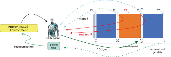
An approximated environment reconstructed from data to simulate radiotherapy adaptation response of patients. A DQN agent manages to extract information from the data of the right‐hand side based on the two transitions (blue‐dashed and red‐solid arrows, explained in Eq. (17) later) and submit actions at the 2/3 period of a treatment (right solid‐green arrow), where the environment is hidden in this illustration. At the end of a whole treatment course, the complete information is then collected for reconstructing the radiotherapy environment (dashed‐green arrow). [Color figure can be viewed at wileyonlinelibrary.com]
2.G.2. Setting for deep reinforcement learning
In DRL, one needs to decide the representation of states, where in our case the states should contain enough patients information to indicate or reflect changes in possible treatment outcomes. In reality, there are numerous variables including hidden ones that may be related to radiotherapy treatment outcomes; it is not feasible to choose all of them. Hence, to develop the transition probabilities, we selected nine variables related to cytokines, SNPs, miRNA, and PET radiomics features in order to predict LC and RP2 (see Table 1) by using the Bayesian network approach developed in Ref. 13 to represent the RAE states. Hence, to develop the transition probabilities, we selected important variables to represent the RAE states for LC and RP2 prediction (see Table 1) based on our previous Bayesian network analysis13 as follows. Firstly, constraint‐based local discovery algorithms using Markov blankets were employed to select the variables that are mostly related to LC or RP2 from the high dimensional dataset (297 candidate variables). Then we built a single Bayesian network from these selected variables for both LC and RP2 prediction by using graph learning algorithms (score‐based learning algorithm and leaf node elimination) with statistical resampling by bootstrapping to mitigate overfitting. Finally, the nodes in the BN with the highest AUC value for joint prediction of LC and RP2 were determined and evaluated using cross‐validation. This process resulted in nine selected features, which included cytokines, SNPs, miRNA, and PET radiomics features that were considered important predictors to represent the state variables.
In this study, we are interested in determining how much dose should be delivered according to patients’ information and thus compute an optimal policy of dose/fraction to mimic/compare with known clinical decisions based on dose adaptation protocols as benchmark for evaluation. This leads us to define the reward (15), as a trade‐off between encouraging improved LC and attempting to suppress RP2. The last term here is meant to comply with the clinical protocol requirement for the probability of RP2 risk not to exceed 17.2%.
Define the state variables with n = 9,
(14) where x1, x2, x5, x6, x9 are cytokines, x3, x4 are of PET radiomics, and x7, x8 are dose features. Let be the allowed actions after t = t * and define our reward function R(s,a) = R(s) based on the complication‐free tumor control (P+) utility25 while respecting the dose escalation clinical protocol requirement:
(15) where s ∈ S, Prob(LC|s) is the conditional probability of obtaining tumor local control after observing state s, similar for Prob(RP2|s).
In the computational aspect of DQN, the Q‐function in Eq. (7) is defined to have a similar form to (4) but with a DNN structure and weights Θ that could be tuned for better approximation of the real Q‐function:
| (16) |
where the inputs and the outputs are adjusted in order to take advantage of deep learning capabilities rather than literally follow (4). We remark that at each state s, another two DNN classifiers were trained for predicting prob (LC|s) and prob (RP2|s) for more accurate computation of the reward (15). Since accurate evaluation of LC and RP2 is also considered as part of the natural transition of the environment that requires as much precision as possible, another two classifiers based on the selected 9 predictors were built to predict the LC and RP2 probabilities trained using the clinical outcomes rather than only the approximation by the LKB model (11). An episode is a sequence of states performed by an agent according to a developed policy π. The termination of an episode was set to invoke whenever Prob(LC|s) > 70% and Prob(RP2|s) < 17.2% are attained.
2.G.3. Setting for probability transition function and building the radiotherapy artificial environment (RAE)
The reconstruction of the RAE then relies on a well‐approximated transition function from the dataset. For this purpose, our data of NSCLC of N = 114 patients are organized in the following form,
where denotes the ith patient at the kth period of treatment with n predictors, i = 1,…,N. k = 0 denotes the period of the treatment t = 0∼week 2; k = 1 is t = week 2∼week 4 and k = 2 stands for t = week 4∼week 6. In full expansion, the data corresponding to Fig. 5 has the form of table with 3 blocks:
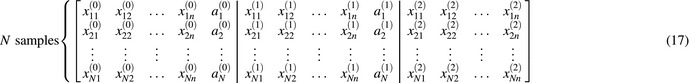
An approximate transition probability trained by a DNN indicates the probability transforming from an old state s to a new states t under action a: . The training was performed by state transitions from different patients and two time periods (pre‐ and during radiotherapy) (k = 0,1) with a total sample size of twice the size of the patients.
| (18) |
with served as labels in the loss function
| (19) |
where y DNN is a set of DNN classifiers to simulate . In our pilot DNN simulations, we observed that the range of state variables has large variations from one another and a single network architecture did not provide satisfying predictions. Thus, to achieve better approximation, we employed n = 9 sets of independent DNNs, denoted by DNN1,DNN2,…,DNN9, to predict the i th variable with its own DNN i such that the ensemble prediction of all variables would yield . By doing this, we were able to calculate the corresponding probabilities of next possible states as the product of each separate variable's transition probability.
Furthermore, to increase the credibility of the Q‐function evaluation based upon the Bellman's iteration (5), we searched up to N possible = 100 next possible transitions via top probabilities of y DNN to distribute possible Q‐values visualized in Fig. 6 (right) where each layer displays the 100 most possible moves under any given action. For comparison with board games, it worth noting that in chess, the possible number of moves is around 20 for the average position while in GO it is about 200.
Although the Bayesian network may provide some constraints on the state transitions, for the majority in our fully connected neural network, there is no obvious causal relationship between state variables x i that could be proven. Therefore, we only considered independent DNNs instead of recurrent neural network approaches.35 Our design of the transition function is shown in Fig. 6.
2.G.4. Setting for generative adversarial network (GAN)
To generate necessary patient sample size for the training of the transition probability function, we chose a feature space containing 3 periods of a treatment plan altogether:
and define a prior latent space equipped with multivariate normal distribution where μ = 0 and Σ = 0.05·I are used. With the completed settings of GAN + transition DNN + DQN, our framework for lung dose adaptation is depicted by Fig. 5.
3. Experiments and results
3.A. Model architecture and computational performance
Each DNN of , i = 1,…,9 in y DNN contains two hidden layers with exponential linear unit (eLU) activations16 and softmax for output layer such that the topology resulted in [n,60,60,n levels], where n levels denotes the number of category variables being discretized. Particularly, we took n levels = 3 since according to Ref. 13 the best prediction falls within range denoting the low, mid, or high value of a given predictor. All DNNs were trained with random dropouts in neurons to avoid overfitting pitfalls. The DNN of the DQN is equipped with two hidden layers in eLU activation functions with topology . Training operations for the DNNs under the described structure utilized the ADAM optimizer, which is a first‐order gradient‐based optimization of stochastic objective functions using adaptive estimates of lower‐order moments.36 In our case, the GAN training took roughly 7,000 epochs with two batches for generating synthetic data; the transition DNN training took 35,000 iterations and the DQN learning ran 30,000–50,000 iterations. Our deep learning algorithms are based on Tensorflow.37 All experiments were implemented in ARC‐TS high‐performance computer cluster (FLUX) with 6 NVIDIA K40 GPUs.
3.B. Results
3.B.1. Generated adversarial network
With the setting of Section 2.G.4, 4,000 new patients were synthesized based on the original data by GAN, which attempts to infer the probability distribution of patients characteristics from limited sample size. As an unsupervised learning method, we measured the GAN performance using the loss function (3) and analyzed the data similarity between the original clinical data and the generated ones as shown in the histograms of Fig. 7. The results show good agreement between our original and synthesized patients characteristics based on the selected nine variables.
Figure 7.

Each subfigure demonstrates approximate probability distribution of a predictor x i , i = 1∼9 by its histogram. Blue‐shaded areas represent the distributions of the original data, while the green‐shaded areas represent the distributions of the generated data by GAN. [Color figure can be viewed at wileyonlinelibrary.com]
3.B.2. The transition probability function of radiotherapy artificial environment
With the generated patient data provided by GAN, the transition probability function of nine discretized chosen variables could be trained more reliably. We predicted each variable interaction independently as mentioned in Section 2.G.3 such that an ensemble DNN classifier would represent the radiotherapy artificial environment with its inputs and outputs given by:
| (20) |
where the cross‐entropy loss function of multiclass prediction was adopted for training:
| (21) |
Using a total sample size of 4,114 with 35,000 iterations for each batch, the following average accuracy for each predictor on 10‐fold cross‐validation was obtained as shown in Fig. 8 ranging from 0.55–1.0.
Figure 8.

The mean accuracy of each predictor: (y 1,y 2,…,y 9) = (0.88,0.65,0.93,1.00,0.55,0.99,0.83,0.98,0.49) with an error bar visualized. [Color figure can be viewed at wileyonlinelibrary.com]
3.B.3. DQN optimal dose per fraction prediction
For reinforcement learning being neither a pure supervised nor a unsupervised learning method, accurate evaluation of an agent can be quite challenging.10, 38 Following,39 our metric for the DQN agent measures the total rewards collected in each episode (a complete treatment course). Figure 9(a) illustrates the total rewards in 10,000 episodes by our in‐house DQN on a classical game MountainCar for instance, where a well‐defined environment is provided by OpenAI40 for training RL agents. It is observed that most of RL algorithms demonstrate oscillating behavior including DQN, where the RL learner here is demonstrated to be stable and accurate in deriving the rewards. On the other hand, Fig. 9(b) evaluates the total reward of automated dose adaptation collected in 10,000 episodes, which are relatively noisy due to the higher complexity of the radiotherapy environment and the associated uncertainties within several components: the GAN error, the transition probability function, and the joint LC‐RP2 classifier and also the oscillating behavior of the DQN itself.
Figure 9.
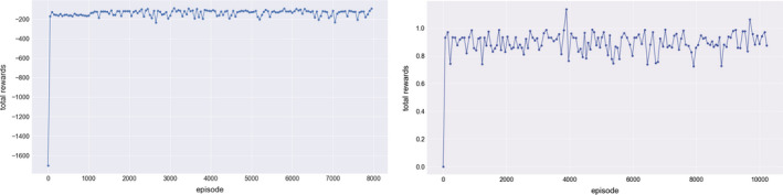
Total rewards of episodes collected by the DQN in two different tasks, where a classical game MountainCar is compared with the artificial environment reconstructed for the dose adaptation. [Color figure can be viewed at wileyonlinelibrary.com]
Dose fraction prediction results are shown in Fig. 10, where the autonomous actions of a(t) in Eq. (9) are computed towards achieving optimal rewards (15) by the DQN to maximize LC rate while minimizing RP2 probability. We allowed the agent to freely control dose from such that Gy are permissible. The DQN algorithm was evaluated on 34 patients from the institutional dose escalation study (UMCC Protocol 2007‐123) who had complete information on the nine selected variables of the RAE. Qualitatively, it is noted that the DQN automatically favored doses between 1.5 and 3.8 Gy, which coincides with the original decision support range of the clinical protocol. This shows the ability of the DQN to learn the effective support interval for treatment adaptation according to the clinical protocols as shown in Fig. 10. Quantitatively, the estimated root‐mean‐square error (RMSE) ≃0.76 Gy, which suggests good agreement with clinical decisions but still has relatively high errors for practical considerations.
Figure 10.
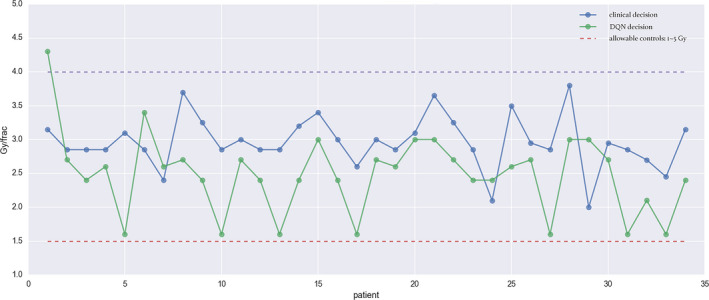
Automated dose decisions given by DQN (green dots) vs. clinical decision (blue dots) with RMSE 0.76 Gy. [Color figure can be viewed at wileyonlinelibrary.com]
However, it was also noted that the DQN decisions based on Eq. (15) were consistently lower than their clinical counterparts. Notably, a manual translation by about 0.75 Gy to all automated dose can achieve a better agreement in RMSE. Besides using a manual constant shift, a natural way to better mimicking the clinical actions is to appropriately modify the reward function by emphasizing higher local control beyond the baseline P+ function as follows:
| (22) |
with w = 0.8. This reward function mainly increases the weight on LC due to with RP2 weighting remained unchanged. As a result, most of doses were escalated to achieve higher LC rate as shown in Fig. 11 achieving an RMSE = 0.5 Gy. Moreover, by considering the knowledge of final outcomes of treatments, we would be able to compare the decisions made by the DQN and those by the clinicians. Under the guiding principle of “doing no harm”, our evaluation criteria is defined in Table 3. Using coloring dots in green and red as indications of “good” and “bad” respectively in Fig. 11, one may identify the quality of the decisions made. As a result, this criteria suggest that the clinician made 19 good and 15 bad decisions, whereas that DQN had 17 good, 4 bad, and 13 potentially good decisions, as organized in Table 2. The results show that there is no significant difference between the clinicians and the DQN in the category of “good” while there exist differences in the category of “bad” and “potentially good”, which may favor the DQN in such uncertain situations. Particularly, this “potentially good” category shown in orange dots of Fig. 11 with (LC, RP2)=(+,−) and reduced dose computed by DQN seems to lower the adaptive dose for decreasing risky situations, which could be partly related to the fact that the actual outcomes were used in training the LC/RP2 predictors. However, this would require further independent validation.
Figure 11.

Automated dose decisions given by DQN (black solid line) vs. clinical decision (blue dashed line) with RMSE = 0.5 Gy. An evaluation of good (green dots), bad (red dots), and potentially good decisions (orange dots) are labeled according to Table 2. [Color figure can be viewed at wileyonlinelibrary.com]
Table 3.
Evaluation of automated dose adaptation, where relative dose ≡ (automated dose − clinical given dose). It should be noted that the notion of good or bad here is quite subjective. For instance, if a patient eventually obtains RP2 without LC, but the DQN suggested higher than the clinical dose given, this is considered as a bad decision. See the row with LC = −, RP2 = + and relative dose > 0
| LC label | RP2 label | Evaluation for clinicians |
|---|---|---|
| + | − | Good |
| + | + | Bad |
| − | + | Bad |
| − | − | Bad |
| LC label | RP2 label | Relative dose | Evaluation for DQN |
|---|---|---|---|
| − | − | ≤ 0 | Bad |
| − | − | > 0.2 | Good |
| − | + | ≥ −0.2 | Bad |
| − | + | < 0.2 | Good |
| + | − | = 0 | Good |
| + | − | > 0 | Bad |
| + | − | < 0 | Potentially good |
| + | + | ≥ 0 | Bad |
| + | + | < 0 | Good |
Table 2.
Summary for the evaluation on clinicians’ and the DQN decisions
| Summary | Good | Bad | Potentially good |
|---|---|---|---|
| clinicians | 19 (55.9%) | 15 (44.1%) | 0 |
| DQN | 17 (50%) | 4 (11.8%) | 13 (38.2%) |
The decisions of the DQN versus the clinicians in Fig. 11 can also be summarized in the boxplots of Fig. 12. The data in the plots were analyzed using two‐tailed Wilcoxon signed‐rank test of paired differences in medians at 5% level of significance.41 For the nonadaptive cases, there was no significant difference between the clinical decisions and the DQN's (P‐value = 0.83). However, in the case of adapted patients there was a difference (P‐value = 0.001). Using one‐tailed analysis it is noted that DQN decisions were generally lower (more conservative) than the clinicians’ with P‐value = 0.0006.
Figure 12.
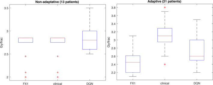
The comparison on 34 patients of protocol 2007‐123 divided into groups with and without adaptation. FX1 denotes the dose/frac given in the first 2/3 period of the treatment; clinical denotes that of the last 1/3 treatment based on protocol 2007‐123 compared with the DQN results using modified reward (20). Note that some patients in FX1 on the left figure were given maximum dose 2.85 Gy/frac according to protocol in Section 2.G.1. [Color figure can be viewed at wileyonlinelibrary.com]
3.B.4. Comparison with temporal difference method
We also compared our proposed approach based on DQN to the traditional RL methods based on TD(0), which is a model‐free approach.9 Among the different TD(λ) techniques, 0 ≤ λ ≤ 1, the TD(0) without eligibility trace used is the closest counterpart to DQN and therefore was chosen for this comparison. The results of TD(0) shown in Fig. 13 are far off from the clinical decisions (RMSE = 3.3 Gy ) in comparison to the DQN suggestions which may be due to the lack of numerical stability in the Q‐value computation. Specifically, this could be attributed to the fact that traditional TD is designed for navigating limited known discrete states in the environment and learn the underlying environment model, whereas the DQN can still determine a possible action even if a state was not previously observed as in the large radiotherapy state space S defined in Eq. (14). Moreover, the generated RAE in our case and inherent replay memory device of DQN contribute to improving the RL stability and convergence, which is not the case in traditional RL.
Figure 13.

Automated dose decisions given by TD(0) method (green dots) vs. clinical decision (blue dots) with RMSE ≃ 3.3 Gy. Possible reasons for the TD method failure to mimic the clinical decisions is the convergence instability. [Color figure can be viewed at wileyonlinelibrary.com]
4. Discussion
In this study, we have explored the feasibility of developing a deep reinforcement learning (DRL) framework for dynamic clinical decision making in adaptive radiotherapy. Reinforcement learning as a different category of machine learning, besides typical supervised and unsupervised learning, has its own prerequisites. A major portion of its development relies on having a well‐defined environment of a Markov Decision Process (MDP), which is a challenge to construct in the case of a complex radiotherapy process with its clinical settings, known experimental constraints, and also limited available datasets to explore such an environment. Therefore, we devised a modified DQN architecture which is neither model‐free nor model‐based, as strictly speaking such approaches would indicate an ability to learn the transition state behavior dynamically during consecutive observations and actions made (e.g., board games), which is not permissible here with the large number of the states and the limited data available. In order to approximate to be sufficiently reliable, the corresponding data for reconstruction must be adequate and usable for training. This problem was tackled in this work by using the GAN approach, which allowed us to generate new synthetic data with characteristics resembling the original limited observations.
In the dataset containing NSCLC of 114 patients who received radiotherapy as part of their treatment and had sufficient (clinical, dosimetric, and biological) information to model RAE, automated dose adaptation by DRL was evaluated on a subset (34 patients) who underwent an institutional dose‐adaptive escalation protocol (UMCC 2007‐123). Our DNNs utilized only two hidden layers, which are developed for our RL application and the corresponding data type, although they are relatively shallower than the Microsoft's Residual Nets or the Google's Inception Net, for instance, especially tasked for image recognition of large dataset. However, more layers (abstraction levels) may be needed as our adaptive radiotherapy datasets grow in terms of variables (‐omics) and sample size.
The reward function in the current work was selected based on prior knowledge and empirical experiences to mimic the clinical adaptation scenario, since the real reward in clinical practice may not be accessible or known. We initially used the reward (15) to derive the suggested dose using the known P+ based utility function and RP2 constraint to mimic the original protocol, which resulted in an RMSE around 0.76 Gy as shown in Fig. 10. However, this reward function resulted in consistent underestimation of the suggested dose (too conservative), and therefore we adjusted the reward function to attain closer policies from the same agent. As suggested by Eq. (21), this adjusted reward function provided higher weights on increasing local control (i.e., raising dose to attain higher LC rates) as shown in Fig. 11. Other possible reward functions are discussed in Ref. 12. The demonstration of how changing rewards would lead to different policies was shown in Figs. 10 and 11. Besides utilizing empirical knowledge to define the reward functions used here, an alternative approach called inverse reinforcement learning (IRL) can be applied to reverse engineer the reward hidden inside the real world based on a perfect mentor,42 which may not be available in practical clinical settings and would be considered as a subject of future work.
Interestingly, we noticed in our results that the DRL not only achieved comparable results to clinical decisions but also can make recommendations that would help adjust current decisions as part of its training when used as a second reader decision support system. The current study has focused on mimicking clinical decisions as a proof‐of‐principle and as validation of the feasibility of DRL for automated dose adaptation applications. However, this algorithm would require further validation on independent datasets once they become available. The use of Bayesian networks as shown here could help constrain the environment as well as define the reward functions. The Bayesian networks not only help predict outcomes but also identify hierarchical relationships within the state variables, which is currently being investigated.
Another limitation of this study is that we only considered a single adaptation action of changing the dose/fraction rather than, for instance, devising a continuous adaptation protocol on a daily or weekly basis. However, this is due to the nature of action information availability within our current data. If one could retrieve more data of tumor response or status monitoring closely/continuously during treatment, this would provide more time stamps to build a more accurate model of RAE and eventually help in reducing the DQN learning error. The information used to reconstruct the RAE environment was limited to certain molecular biomarkers and PET imaging data. However, this information could be further enriched by utilizing tumor and normal tissue response and monitoring indicators from radiogenomics43 or noninvasive new imaging information from CT radiomics,44 advanced ultrasound,45, 46, 47 magnetic resonance spectroscopy,48 or optical imaging in the case of superficial tumors.49 Should more data become available, continuous adaptive decision‐making may be introduced and further evaluated using the proposed DRL approach.
5. Conclusions
Our study introduced deep RL as a viable solution for response‐adaptive clinical decision making. We proposed a combination of three deep learning components: GAN + transition DNN + DQN to provide an automated dose adaptation framework as shown in Fig. 1(b). All three components are essential and complementary to each other‐ from generating the necessary training data for learning the transition probability of the approximated environment to searching for the optimal actions. The use of deep Q‐networks as a modern reinforcement learning technique allows us to potentially realize automated decision making in complex clinical environments such as radiotherapy. Towards this goal, we approximated the transition probability function from historical treatment plans via independent DNNs and GAN to generate sufficient synthetic patient data for training. Our proposed method was demonstrated successfully on an institutional dose escalation study with empirical reward functions. However, further developments and validations on larger multi‐institutional datasets are still required for building an autonomous clinical decision support system for response‐based adaptive radiotherapy.
Conflict of Interest
The authors have no relevant conflicts of interest to disclose.
Acknowledgments
The authors thank Dr. Kong and Dr. Jolly for their help in providing the lung testing datasets for the study and Julia Pakela for the careful proofreading of our manuscript. This work was supported in part by the National Institutes of Health P01 CA059827.
References
- 1. Jaffray DA. Image‐guided radiotherapy: from current concept to future perspectives. Nat Rev Clin Oncol. 2012;9:688–699. [DOI] [PubMed] [Google Scholar]
- 2. Eisbruch A, Lawrence TS, Pan C, et al. Using FDG‐PET acquired during the course of radiation therapy to individualize adaptive radiation dose escalation in patients with non‐small cell lung cancer.
- 3. Kong F, Ten Haken RK, Schipper M, et al. Effect of midtreatment PET/CT‐adapted radiation therapy with concurrent chemotherapy in patients with locally advanced nonsmall‐cell lung cancer: a phase 2 clinical trial. JAMA Oncol. 2017;3:1358. [DOI] [PMC free article] [PubMed] [Google Scholar]
- 4. Bradley JD, Paulus R, Komaki R, et al. Standard‐dose versus high‐dose conformal radiotherapy with concurrent and consolidation carboplatin plus paclitaxel with or without cetuximab for patients with stage iiia or iiib non‐small‐cell lung cancer (RTOG 0617): a randomised two‐by‐two factorial phase 3 study. Lancet Oncol. 2015;16:187–199. [DOI] [PMC free article] [PubMed] [Google Scholar]
- 5. Naqa IEl, Li R, Murphy MJ, et al. Machine learning in radiation oncology. In: Theory and Applications. New York, NY: Springer International Publishing. [Google Scholar]
- 6. LeCun Y, Bengio Y, Hinton G. Deep learning. Nature. 2015;521:436–444. [DOI] [PubMed] [Google Scholar]
- 7. Dalm MU, Litjens G, Holland K, et al. Using deep learning to segment breast and fibroglandular tissue in MRI volumes. Med Phys. 2017;44:533–546. [DOI] [PubMed] [Google Scholar]
- 8. Ibragimov B, Xing L. Segmentation of organs‐at‐risks in head and neck CT images using convolutional neural networks. Med Phys. 2017;44:547–557. [DOI] [PMC free article] [PubMed] [Google Scholar]
- 9. Sutton RS, Barto AG. Reinforcement Learning: An Introduction. Vol 1. Cambridge: MIT Press; 1998. [Google Scholar]
- 10. Mnih V, Kavukcuoglu K, Silver D, et al. Playing Atari with deep reinforcement learning. arXiv preprint arXiv:13125602 2013.
- 11. Kim M, Ghate A, Phillips MH. A Markov decision process approach to temporal modulation of dose fractions in radiation therapy planning. Phys Med Biol. 2009;54:4455. [DOI] [PubMed] [Google Scholar]
- 12. Vincent RD, Pineau J, Ybarra N, et al.. Chapter 16: practical rein‐forcement learning in dynamic treatment regimes. In: Adaptive Treatment Strategies in Practice. Philadelphia, PA: Society for Industrial and Applied Mathematics; 2015:263–296. [Google Scholar]
- 13. Luo Y, Naqa IEl, McShan DL, et al. Unraveling biophysical interactions of radiation pneumonitis in non‐small‐cell lung cancer via Bayesian network analysis. Radiother Oncol. 2017;123:85–92. [DOI] [PMC free article] [PubMed] [Google Scholar]
- 14. Vallieres M, Freeman CR, Skamene SR, et al. A radiomics model from joint FDG‐PET and MRI texture features for the prediction of lung metastases in soft‐tissue sarcomas of the extremities. Phys Med Biol. 2015;60:5471–5496. [DOI] [PubMed] [Google Scholar]
- 15. Naqa IEl. The role of quantitative pet in predicting cancer treatment outcomes. Clin Translat Imag. 2014;2:305–332. [Google Scholar]
- 16. Clevert D‐A, Unterthiner T, Hochreiter S. Fast and accurate deep network learning by exponential linear units (elus). arXiv preprint arXiv:151107289 2015.
- 17. Vapnik V. The Nature of Statistical Learning Theory. Berlin: Springer Science & Business Media; 2013. [Google Scholar]
- 18. Hornik K, Stinchcombe M, White H. Multilayer feedforward networks are universal approximators. Neural Netw. 1989;2:359–366. [Google Scholar]
- 19. Srivastava N, Hinton GE, Krizhevsky A, et al. Dropout: a simple way to prevent neural networks from overfitting. J Mach Learn Res. 2014;15:1929–1958. [Google Scholar]
- 20. Goodfellow I, Pouget‐Abadie J, Mirza M, et al. Generative adversarial netsIn Advances in Neural Information Processing Systems; 2014:2672–2680.
- 21. Mohri M, Rostamizadeh A, Talwalkar A. Foundations of Machine Learning. Cambridge: The MIT Press; 2012. [Google Scholar]
- 22. Mnih V, Kavukcuoglu K, Silver D, et al. Human‐level control through deep reinforcement learning. Nature. 2015;518:529–533. [DOI] [PubMed] [Google Scholar]
- 23. Tsitsiklis JN, Van Roy B. Analysis of temporal‐diffference learning with function approximation. inAdvances in neural information processing systems; 1997:1075–1081
- 24. Kutcher GJ, Burman C. Calculation of complication probability factors for non‐uniform normal tissue irradiation: the effective volume method gerald. Int J Radiat Oncol Biol Phys. 1989;16:1623–1630. [DOI] [PubMed] [Google Scholar]
- 25. gren A, Brahme A, Turesson I. Optimization of uncomplicated control for head and neck tumors. Int J Radiat Oncol Biol Phys. 1990;19:1077–1085. [DOI] [PubMed] [Google Scholar]
- 26. Ramírez MF, Huitink JM, Cata JP. Perioperative clinical interventions that modify the immune response in cancer patients. Open J Anesthesiol 2013;3:133. [Google Scholar]
- 27. Schaue D, Kachikwu EL, McBride WH. Cytokines in radiobiological responses: a review. Radiat Res. 2012;178:505–523. [DOI] [PMC free article] [PubMed] [Google Scholar]
- 28. Warltier DC, Laffey JG, Boylan JF, et al. The systemic inflammatory response to cardiac surgeryimplications for the anesthesiologist. J Am Soc Anesthesiol. 2002;97:215–252. [DOI] [PubMed] [Google Scholar]
- 29. Galloway MM. Texture analysis using gray level run lengths. Comput Graph Image Process. 1975;4:172–179. [Google Scholar]
- 30. Deshmane SL, Kremlev S, Amini S, et al. Monocyte chemoattractant protein‐1 (MCP‐1): an overview. J Interferon Cytokine Res. 2009;29:313–326. [DOI] [PMC free article] [PubMed] [Google Scholar]
- 31. Nguyen D‐HT, Stapleton SC, Yang MT, et al. Biomimetic model to reconstitute angiogenic sprouting morphogenesis in vitro. Proc Natl Acad Sci USA. 2013;110:6712–6717. [DOI] [PMC free article] [PubMed] [Google Scholar]
- 32. Letterio JJ, Roberts AB. Regulation of immune responses by TGF‐β . Ann Rev Immunol. 1998;16:137–161. [DOI] [PubMed] [Google Scholar]
- 33. Bentzen SM, Dische S. Morbidity related to axillary irradiation in the treatment of breast cancer. Acta Oncolog. 2000;39:337–347. [DOI] [PubMed] [Google Scholar]
- 34. Søvik Å, Ovrum J, Rune Olsen D, et al. On the parameter describing the generalised equivalent uniform dose (gEUD) for tumours. Phys Med. 2007;23:100–106. [DOI] [PubMed] [Google Scholar]
- 35. Goller C, Kuchler A. Learning task‐dependent distributed representations by backpropagation through structure. in IEEE International Conference on Neural Networks. Vol 1. IEEE; 1996:347–352. [Google Scholar]
- 36. Kingma D, Ba J. Adam: A method for stochastic optimization. arXiv preprint arXiv:1412698 2014.
- 37. Abadi M, Agarwal A, Barham, P , et al. TensorFlow: Large‐scale machine learning on heterogeneous systems. 2015. software available from tensorflow.org
- 38. Brockman G, Cheung V, Pettersson L, et al. OpenAI Gym; 2016. arXiv:160601540.
- 39. Bellemare MG, Naddaf Y, Veness J, et al. The arcade learning environment: an evaluation platform for general agents. J Artif Intell Res(JAIR). 2013;47:253–279. [Google Scholar]
- 40. Oh JH, Craft J, Lozi RAl, et al. A Bayesian network approach for modeling local failure in lung cancer. Phys Med Biol. 2011;56:1635. [DOI] [PMC free article] [PubMed] [Google Scholar]
- 41. Lowry R. Concepts and applications of inferential statistics; 2014.
- 42. Ng AY, Russell SJ, et al. Algorithms for inverse reinforcement learning. in ICML; 2000:663–670.
- 43. Naqa IEl, Kerns SL, Coates J, et al. Radiogenomics and radiotherapy response modeling. Phys Med Biol. 2017;62:R179. [DOI] [PMC free article] [PubMed] [Google Scholar]
- 44. Goh V, Ganeshan B, Nathan P, et al. Assessment of response to tyrosine kinase inhibitors in metastatic renal cell cancer: CT texture as a predictive biomarker. Radiology. 2011;261:165–171. [DOI] [PubMed] [Google Scholar]
- 45. Sadeghi‐Naini A, Papanicolau N, Falou O, et al. Low‐frequency quantitative ultrasound imaging of cell death in vivo. Med Phys. 2013;40:082901. [DOI] [PubMed] [Google Scholar]
- 46. Falou O, Sadeghi‐Naini A, Prematilake S, et al. Evaluation of neoadjuvant chemotherapy response in women with locally advanced breast cancer using ultrasound elastography. Translat Oncol. 2013;6:17–24. [DOI] [PMC free article] [PubMed] [Google Scholar]
- 47. Sadeghi‐Naini A, Papanicolau N, Falou O, et al. Quantitative ultrasound evaluation of tumor cell death response in locally advanced breast cancer patients receiving chemotherapy. Clin Cancer Res. 2013;19:2163–2174. [DOI] [PubMed] [Google Scholar]
- 48. Witney TH, Kettunen MI, Hu DE, et al. Detecting treatment response in a model of human breast adenocarcinoma using hyperpolarised [1‐13C] pyruvate and [1, 4‐13C2] fumarate. Brit J Cancer. 2010;103:140. [DOI] [PMC free article] [PubMed] [Google Scholar]
- 49. Sadeghi‐Naini A, Vorauer E, Chin L, et al. Early detection of chemotherapy‐refractory patients by monitoring textural alterations in diffuse optical spectroscopic images. Med Phys. 2015;42:6130–6146. [DOI] [PubMed] [Google Scholar]