Accelerated Phase Contrast Flow Imaging With Direct Complex Difference Reconstruction

Abstract

Purpose

To propose and evaluate a new model-based reconstruction method for highly accelerated phase-contrast magnetic resonance imaging (PC-MRI) with sparse sampling.

Theory and Methods

This work presents a new constrained reconstruction method based on low-rank and sparsity constraints to accelerate PC-MRI. More specifically, we formulate the image reconstruction problem into separate reconstructions of flow-reference image sequence and complex differences. We then utilize the joint partial separability and sparsity constraints to enable high quality reconstruction from highly undersampled (k, t)-space data. We further integrate the proposed method with ESPIRiT based parallel imaging model to effectively handle multichannel acquisition.

Results

The proposed method was evaluated with in vivo data acquired from both 2D and 3D PC flow imaging experiments, and compared with several state-of-the-art methods. Experimental results demonstrate that the proposed method leads to more accurate velocity reconstruction from highly undersampled (k, t)-space data, and particularly superior capability of capturing the peak velocity of blood flow. In terms of flow visualization, blood flow patterns obtained from the proposed reconstruction also exhibit better agreement with those obtained from the fully sampled reference.

Conclusion

The proposed method achieves improved accuracy over several state-of-the-art methods for velocity reconstruction with highly accelerated (k, t)-space data

INTRODUCTION

Phase-contrast magnetic resonance imaging (PC-MRI) is a noninvasive imaging technique that acquires time-resolved velocity information of blood flow (1–3). It not only enables visualization of complex blood flow dynamics in 3D (4,5), but also allows for measurement of flow volumes and various hemodynamic parameters, including wall shear stress (6–8), pressure gradients (9–11), and pulse wave velocity (12,13). Over the past few decades, PC-MRI has demonstrated great promise in understanding and diagnosis of cardiovascular pathologies, such as atherosclerosis (4), aneurysms (14,15), and arteriovenous malformation (16).

PC-MRI measures the blood flow velocity at each encoding direction from the phase difference between a flow-reference data set and flow-encoded data set. To acquire three directional flow information, four sets of data have to be acquired, which often leads to prolonged acquisition times (3). For example, acquisition time for a standard 3D PC-MRI experiment for aortic arch is around 20–30 min (4), significantly hindering its use for clinical practice.

A number of fast imaging techniques have been developed to accelerate PC-MRI. Advanced non-Cartesian pulse sequences based on radial (17) and spiral (18,19) acquisitions have been proposed to improve imaging speed for PC-MRI. Parallel imaging techniques, such as sensitivity encoding (SENSE) (20) or generalized autocalibrating partially parallel acquisitions (GRAPPA) (21), utilizing multiple receiver coils can provide a 2× or 3× acceleration for clinical PC-MRI. These methods have been further extended to the (k, t) domain to leverage spatiotemporal correlation of dynamic images for higher undersampling levels. For example, k-t Broad-use Linear Acquisition Speed-up Technique (k-t BLAST)/k-t SENSE (22) was developed and applied to accelerate flow measurements in carotid bifurcation (23) with up to 5× acceleration. k-t GRAPPA (24,25) and k-t iterative self-consistent parallel imaging reconstruction, i.e., k-t SPIRiT (26), respectively extending the k-space parallel imaging reconstruction, have also been applied to PC-MRI for aortic arch. Alternatively, compressed sensing (CS) techniques, including sparsity (27,28) and low-rank based reconstruction methods (29–34), have been developed to utilize low dimensional representations of dynamic images to enable image reconstruction from highly undersampled (k, t)-space data. Some of these methods have been extended to accelerate PC-MRI (e.g., (35–39)).

Due to the velocity encoding scheme, flow-reference and flow-encoded datasets are often highly correlated (e.g., they often share very similar magnitude images though their phases are different). As a result, the complex differences, obtained by subtracting the flow-reference from flow-encoded data, generally admit parsimonious representations (e.g., sparsity and low-rankedness properties), which can be leveraged to enable sparse sampling. A number of methods have been developed to utilize the underlying signal characteristics of complex differences to accelerate PC-MRI. For example, Ref. (38) incorporated the sparsity constraint of complex differences into the reconstruction, while Ref. (36) used the partial separability or low-rank constraint to reconstruct the complex differences.

In this work, we propose a new model-based reconstruction method to accelerate PC-MRI. With a variable-density sampling scheme, the proposed method enables separate reconstruction of flow-reference image sequence and complex differences associated with different velocity encoding directions. The resulting undersampled reconstruction problems are solved by jointly enforcing the partial separability and sparsity constraints (34). Furthermore, we incorporate the proposed method with ESPIRiT based parallel MRI model (40) to handle multi-coil data. The proposed formulation results in a convex optimization problem, which is then solved by an algorithm based on the half-quadratic regularization with continuation. The proposed method was systematically evaluated using both 2D and 3D in vivo PC-MRI data. Its superior performance over several state-of-the-art methods will be demonstrated.

THEORY

The discrete imaging equation for PC-MRI can be written as

$${\mathbf{d}}_{v,i}=\mathrm{\Omega }({\mathbf{F}}_s{\mathbf{S}}_i{\mathbf{C}}_v)+{\mathbf{n}}_{v,i},$$ [1]

where

$${\mathbf{C}}_v=\left[\begin{array}{ccc}{I}_1^v\left({\mathbf{x}}_1\right)& \cdots & I_T^v\left({\mathbf{x}}_1\right)\\ ⋮& \ddots & ⋮\\ I_1^v\left({\mathbf{x}}_N\right)& \cdots & I_T^v\left({\mathbf{x}}_N\right)\end{array}\right]$$ [2]

denotes the Casorati matrix (29) for the flow-reference image sequence (i.e., v = 1) or the velocity-encoded image sequence (i.e., v = 2, …, 4), d_v;i the measured data acquired at the ith receiver coil and vth flow encoding direction, S_i the sensitivity map for the ith coil, F_s the spatial Fourier transform matrix, Ω the undersampling operator, and n_v;i measurement noise. The problem is to accurately reconstruct C_v from highly undersampled (k, t)-space data ${\left\{{\mathbf{d}}_v\right\}}_{v=1}^4$, and then extract the velocity information.

Here, we present a model-based reconstruction method to address this problem. The proposed method employs a variable-density sampling scheme, as illustrated in Figure 1, which fully samples the central region of (k, t)-space while sparsely sampling other regions. Furthermore, it applies the same sampling pattern for both flow-reference and flow-encoded image sequences. With this acquisition strategy, reconstruction of flow-reference image sequence and complex differences can be decoupled. More specifically, the proposed method can be summarized in the following three steps: i) reconstructing the flow-reference image sequence, ii) reconstructing the complex-difference image sequences, and iii) extracting the phase difference or velocity information. In Figure 1, we present an overview of the proposed method, and the rest of this section will describe each step in detail.

FIG. 1.

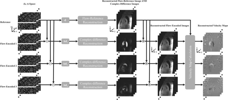
Schematic workflow of the proposed method. Note that it performs separate reconstruction of flow-reference images and complex differences with low-rank and sparsity constraints, after which the phase differences, or the velocity information, are extracted.

Reconstruction of Flow-Reference Image Sequence

We first reconstruct the flow-reference image sequence C₁ from undersampled (k, t)-space data {d_1;i} Note that the flow-reference image sequence often shares similar image characteristics (e.g., spatial-spectral sparsity, spatiotemporal correlation, and low-rankedness) to dynamic imaging sequences in cardiac imaging or other dynamic imaging applications. Therefore, it could be reconstructed using one of the existing (k, t)-domain undersampled reconstruction methods as reviewed previously. Here, we apply a joint partial separability and sparsity based reconstruction method (34,41) to determine C₁. More specifically, we impose a partial separability, or low-rank constraint, on C₁ through the following matrix factorization: C = U_sV_t (29,31,32), where ${\mathbf{U}}_s\in {ℂ}^{N\times L}$denotes the spatial subspace of C₁, V_t is the temporal subspace of C₁, and L refers to the rank. Moreover, we pre-estimate V_t from the fully sampled central (k, t)-space data as described in (29,30) and enforce the spatial-spectral sparsity constraint to regularize the ill-conditioned inverse problem. To effectively utilize multichannel acquisition, we integrate the proposed image model with the ESPIRiT based parallel imaging model (40), in which a “soft” SENSE based formulation is used to improve the robustness to the estimated coil sensitivities. Putting together these components, the reconstruction problem can be formulated as

$$<{\widehat{\mathbf{U}}}_{\mathrm{s}}^1,\dots ,{\widehat{\mathbf{U}}}_{\mathrm{s}}^M>=\arg \underset{{\mathbf{U}}_{\mathrm{s}}^1,\dots ,{\mathbf{U}}_{\mathrm{s}}^M\in {ℂ}^{N\times L}}{min}{{\displaystyle \sum _{i=1}^{N_c}\Vert {\mathbf{d}}_{1,i}-\mathbf{\Omega }\left[{\mathbf{F}}_{\mathrm{s}}{\displaystyle \sum _{j=1}^M{\mathbf{S}}_i^j\left({\mathbf{U}}_{\mathrm{s}}^j{\mathbf{V}}_t\right)}\right]\Vert }}_2^2+{\mathrm{\lambda }}_1{\displaystyle \sum _{j=1}^M{\Vert \text{vec}\left({\mathbf{U}}_{\mathrm{s}}^j{\mathbf{V}}_{\mathrm{f}}\right)\Vert }_1,}$$ [3]

where ${\left\{{\mathbf{S}}^j\right\}}_{j=1}^M$denotes M sets of sensitivity maps estimated from the temporally averaged central k-space data using the ESPIRiT method, ${\mathbf{U}}_{\mathrm{s}}^j(j=1,\dots ,M)$ represents the associated spatial coefficients, V_f is the temporal Fourier transform of V_t, λ refers to the regularization parameter, and vec(·) denotes the operator concatenating the columns of a matrix. Note that Eq. [3] is a convex optimization problem, for which we present an algorithm based on the half-quadratic regularization with continuation (34) (the algorithmic detail can be found in Appendix). After reconstructing ${\mathbf{U}}_{\mathrm{s}}^j\left(j=1,\dots ,M\right)$, C₁ can be reconstructed through the coil combination of M coil images, i.e., ${\displaystyle {\sum }_{j=1}^M{\mathbf{S}}_i^j{\mathbf{U}}_{\mathrm{s}}^j{\mathbf{V}}_{\mathrm{t}}}$.

Reconstruction of Complex Differences

Given that the same sampling strategy is used for both flow-reference and flow-encoded image sequences, complex differences can be directly reconstructed from the residual (k, t)-space data Δd_i;v obtained by subtracting (k, t)-space data associated with the flow-reference image sequence from that associated with the flow-encoded image sequence. Considering that the flow-reference and flow-encoded image sequences are highly correlated, complex differences often have lower-dimensional structures. For example, it admits a sparse representation in the spatiotemporal domain. Moreover, it can also be well approximated using a partially separable (or low-rank) model. Here, we again use the joint partial separability and sparsity based reconstruction method to directly reconstruct the complex differences from the residual (k, t)-space data. Instead of imposing a spatial-spectral sparsity constraint, we impose the sparsity constraint on the spatial coefficients of the temporal basis functions, motivated by the fact that complex differences often have limited spatiotemporal support structure. We further estimate the temporal subspace ΔV_t;i associated with the complex differences from the central region of residual (k, t)-space data. With the same set of sensitivity maps calculated from the first step, the complex-difference reconstruction problem can be formulated as

$$<\Delta {\widehat{\mathbf{U}}}_{\mathrm{s}}^1,\dots ,\Delta {\widehat{\mathbf{U}}}_{\mathrm{s}}^M>=\arg \underset{\Delta {\mathbf{U}}_{\mathrm{s}}^1,\dots ,\Delta {\mathbf{U}}_{\mathrm{s}}^M\in {ℂ}^{N\times L}}{min}{{\displaystyle \sum _{i=1}^{N_c}\Vert \Delta {\mathbf{d}}_{v,i}-\mathbf{\Omega }\left[{\mathbf{F}}_{\mathrm{s}}{\displaystyle \sum _{j=1}^M{\mathbf{S}}_i^j\left(\Delta {\mathbf{U}}_{\mathrm{s}}^j\Delta {\mathrm{V}}_t\right)}\right]\Vert }}_2^2+\mathrm{\mu }{\displaystyle \sum _{j=1}^M\text{TV}\left(\Delta {\mathbf{U}}_{\mathrm{s}}^j\right),}$$ [4]

where ΔU_s spans the spatial subspace for the complex-difference sequence. The above optimization problem can be solved using a similar convex optimization algorithm which is described in detail in Appendix.

Reconstruction of Phase Difference

With the reconstructed flow-reference image sequence and complex differences, the phase difference for three directions can be calculated as $\angle \left(\Delta {\widehat{\mathbf{U}}}_{\mathrm{s}}\Delta {\mathbf{V}}_{\mathrm{t}}+{\widehat{\mathbf{U}}}_{\mathrm{s}}{\mathbf{V}}_{\mathrm{t}}\right)-\angle {\widehat{\mathbf{U}}}_{\mathrm{s}}{\mathbf{V}}_{\mathrm{t}}$ which is proportional to the blood flow velocities.

METHODS

Data Acquisition

We first evaluated the performance of the proposed method with 2D in vivo retrospectively undersampled PC-MRI data in which reconstruction from the fully sampled data was treated as the underlying reference. The experiments were performed on a 3.0 T whole-body MR scanner (Achieva, Philips Medical System, Best, The Netherlands) with a 32-channel cardiovascular coil. A prospectively electrocardiogram (ECG)-triggered cine gradient-echo sequence was used in data acquisition. Six healthy volunteers (mean age: 25, range: 23–28) participated in the experiments with the informed written consent. A sagittal slice across the ascending aorta, aortic arch, and descending aorta was imaged with three-directional velocity encodings in the AP (anterior-to-posterior), FH (foot-to-head), and RL (right-to-left) directions. The relevant imaging parameters include: field of view (FOV) 176 × 260 mm² (FH/RL), slice thickness = 5 mm, spatial resolution = 2.6 × 2.6 mm² (FH/RL), flip angle = 5°, repetition/echo time (TR/TE) = 6.2 ms/2.2 ms, number of cardiac phases = 32, and encoding velocity (VENC) = 150 cm/s. The temporal resolution is approximately 28 ms. To reduce respiratory motion artifacts, three averages were performed for the acquisition of the fully sampled dataset, resulting in an average total scan duration of 402 s. The fully sampled 2D cine PC-MRI data were retrospectively undersampled with three net acceleration factors (i.e., R = 4, 6, and 8) using the sampling scheme shown in Figure 1. The acquired central (k, t)-space regions were adjusted according to each applied acceleration factor. As required by the reconstruction scheme, the four sets of PC-MRI data, including one set of flow-reference and three sets of flow-encoded data, share the same sampling pattern.

We also evaluated the performance of the proposed method for both 3D retrospectively and prospectively undersampled experiments. For the retrospectively under-sampled experiments, we conducted the whole aortic, ECG-triggered PC-MRI experiments on six healthy volunteers (mean age: 26, range: 23–30). The related imaging parameters include: FOV = 180 × 270 × 56 mm³ (FH/RL/AP) with a voxel size of 2.8 × 2.8 × 2.8 mm³, flip angle = 5°, VENC = 150 cm/s, and the number of cardiac phases = 28, and TR = 4.0 ms. Scan time for the fully sampled data was 26 min at an averaged heart rate of 72 beats/min. Here we performed the retrospective undersampling with two net acceleration factors (i.e., R = 4 and 8). For the prospectively undersampled experiments, the same acquisition parameters were applied as the retrospective experiments, and here we used the net acceleration factor of 8. Again, six subjects were scanned for this set of experiments.

Implementation

We estimated the coil sensitivity maps for the proposed method from the temporally averaged central (k, t)-space data using ESPIRiT. We selected the size of the calibration region along phase-encoding direction to be 14, and the kernel size to be 6 × 6, which consistently yield a good tradeoff between the reconstruction accuracy and computational efficiency. Furthermore, we used two sets of sensitivity maps (i.e., M = 2) in our reconstruction to reduce artifacts caused by motion. After reconstruction, phase correction (42) was performed to correct the phase offsets caused by eddy currents.

We compared the performance of proposed method, which integrates the complex difference constraint with the joint partial separability and sparsity reconstruction framework (named PS-CD-SPARSE), with two state-of-the-art reconstruction methods, k-t SPARSE (37) and PS-SPARSE (34). Note that for the two competing methods, each flow-encoded image sequence was reconstructed separately, after which the velocity information was extracted. We manually selected the model orders and/or regularization parameters for all the methods to optimize their performance.

Data Analysis and Visualization

We performed the quantitative analysis to evaluate the accuracy of different reconstruction methods. Specifically, we manually drew a region of interest (ROI) for both the ascending aorta (AAo) and descending aorta (DAo), for which we define the root-mean-square-error (RMSE) as

$$\mathbf{RMSE}=\sqrt{\frac{{\displaystyle {\sum }_{t=1}^{N_t}{\displaystyle {\sum }_{i\in \text{ROI}}{\left|v_{t,i}^r-v_{t,i}^o\right|}^2}}}{{\displaystyle {\sum }_{t=1}^{N_t}{\displaystyle {\sum }_{i\in \text{ROI}}{\left|v_{t,i}^o\right|}^2}}}}$$ [5]

to assess the accuracy of flow measurements, where $v_{t,i}^r$ and $v_{t,i}^o$ respectively denote the velocity at time t for the ith voxel from the reconstructed and originally fully-sampled measurement over a selected ROI, and N_t denotes the number of cardiac phases. Additionally, we calculated the angle α between the velocity vectors (denoted as $\overrightarrow{v}={\left[v_{AP},v_{FH},v_{RL}\right]}^T$)obtained from the fully sampled and reconstructed data set as

$$\alpha =\frac{1}{N_t}{\displaystyle \sum _{t=1}^{N_t}{\displaystyle \sum _{i\in \text{ROI}}\arccos \frac{{\overrightarrow{v}}_{t,i}^r\cdot {\overrightarrow{v}}_{t,i}^o}{\left|{\overrightarrow{v}}_{t,i}^r\right|\cdot \left|{\overrightarrow{v}}_{t,i}^o\right|}.}}$$ [6]

To examine the temporal fidelity of different reconstruction methods, we plot the average flow velocities within two ROIs in AAo and DAo over the entire cardiac cycle. We also performed a linear regression analysis on the velocity data reconstructed from fully sampled and undersampled datasets, and calculated the Pearson’s correlation coefficients. The above statistical analysis was done with the six subjects. For the flow visualization, GT-Flow (GyroTools LLC, Switzerland) was used to automatically segment the aorta and generate the pathline visualization of the flow field for the 3D experiments.

RESULTS

2D Experiments

We first illustrate the reconstruction accuracy of different methods for reconstructing PC-MRI images. Figure 2 shows the reconstructed complex differences (CD) of one systolic cardiac phase using k-t SPARSE, PS-SPARSE, and PS-CD-SPARSE for one volunteer. For k-t SPARSE and PS-SPARSE, the CD images were obtained by subtracting the reconstructed flow-reference image from the reconstructed flow-encoded image, while PS-CD-SPARSE directly generated the CD image from the second step of the proposed reconstruction. As can be seen, the reconstruction errors associated with the CD images obtained from k-t SPARSE and PS-SPARSE increase with higher acceleration factors, while the proposed method better suppresses these discrepancies. Furthermore, the proposed method prevents the residual artifacts of the reconstructed complex differences in the blood vessel compared with k-t SPARSE and PS-SPARSE. The corresponding error maps shown in the figure further confirm that at the high acceleration, PS-CD-SPARSE results in better reconstruction of the CD images than the other two methods. Note that the comparison with PS-SPARSE illustrates the benefits of separate reconstruction of the complex differences.

FIG. 2.

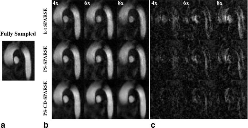
Magnitude of the reconstructed complex differences for a systolic cardiac phase and the associated error maps. a: Reference from the fully sampled data. b: The reconstructed complex differences using k-t SPARSE, PS-SPARSE and PS-CD-SPARSE at the acceleration factors R = 4, 6, 8. c: The error maps associated with the reconstructions in (b).

Figure 3a–c shows the reconstructed velocity maps and corresponding error maps obtained from k-t SPARSE, PS-SPARSE and PS-CD-SPARSE at R = 4, 6, and 8. It can be seen that k-t SPARSE results in a larger error in the velocity measurements under a higher acceleration factor, particularly in the AAo and DAo along FH-direction. In contrast, the velocities reconstructed from PS-CD-SPARSE are more accurate. Figure 3d plots the RMSE of the velocity map within the ROI for the three methods at different acceleration factors. Clearly, the proposed method yields more accurate velocity measurements than the other two methods with highly undersampled data.

FIG. 3.

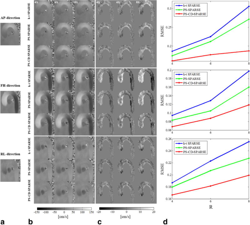
Reconstructed velocity maps for a systolic cardiac phase at different acceleration factors. a: Reference from the fully sampled data along the AP, FH, and RL directions. b: The reconstructed velocity maps using k-t SPARSE, PS-SPARSE, and PS-CD-SPARSE at R = 4, 6, 8. c: The associated velocity error maps with the reconstructions in (b) within the masked ROI. d: The RMSEs for each velocity component.

The reconstructed velocity profiles along the FH-direction through the AAo and DAo are shown in Figure 4. When R = 4, the velocity profiles from all three methods are all close to the one obtained from the fully sampled data. When R is increased to 8, k-t SPARSE and PS-SPARSE result in underestimates of peak velocity. In contrast, PS-CD-SPARSE better captures the velocity of the blood flow over the entire cardiac cycle.

FIG. 4.

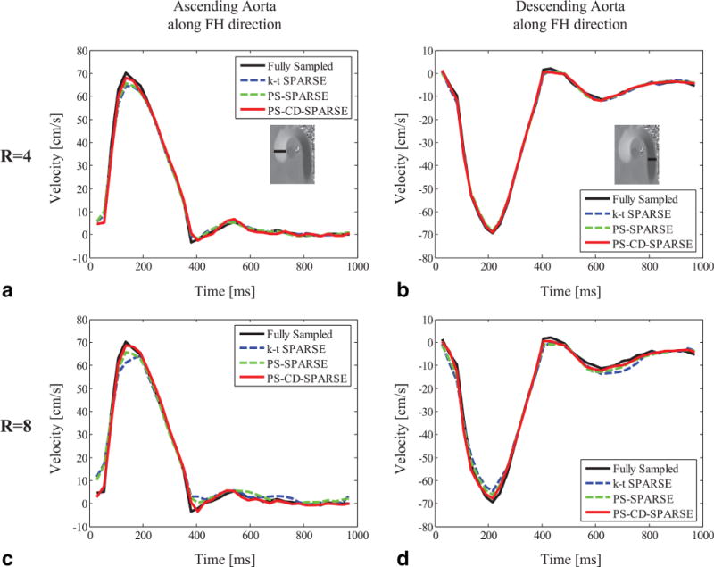
The reconstructed time-resolved velocity profiles through the ascending aorta (AAo) for R = 4 (a) and R = 8 (c) using k-t SPARSE, PS-SPARSE, and PS-CD-SPARSE. The reconstructed velocity profiles through the descending aorta (DAo) at R = 4 (b) and R = 8 (d).

Figure 5 shows the correlation analysis between the reference and reconstructed velocities obtained from three reconstruction methods at R = 4, 6, and 8. To demonstrate the efficacy of the proposed method for different imaging subjects, we calculated the Pearson’s correlation coefficients associated with the linear regression analysis for the six volunteers, which are shown in Supporting Table S1. Moreover, the mean and standard deviation of the RMSE and error angles for the reconstructed velocities for all volunteers are respectively shown in Figure 6a,b. Note that although the errors increase with the higher acceleration, PS-CD-SPARSE constantly yields less errors than the other two methods.

FIG. 5.

(a), (b), and (c) respectively show the pixelwise linear regression of reconstructed velocities from R = 4, 6, and 8 with respect to the reference from the fully sampled data. Note that all three velocity components in the ROI are included in the regression analysis.

FIG. 6.

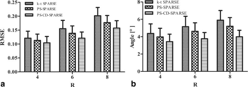
2D retrospectively undersampled experiments. a: Mean and standard deviation for the overall RMSE of the magnitudes of the reconstructed velocities. b: Mean and standard deviation for the angles between the reconstructed velocity vectors and those from the fully sampled data. Note that the above metrics were calculated with respect to the six volunteers and included all the pixels within the ROI.

3D Experiments

Figure 7 shows the pathline visualization of the flow fields obtained from k-t SPARSE, PS-SPARSE, and PS-CD-SPARSE reconstruction under R = 4 and 8 using the particles released at three delay times (i.e., 181.8 ms, 188.2 ms, and 194.6 ms) after the R-wave. As can be seen, the flow pattern from the k-t SPARSE reconstruction significantly deviates from the underlying ground truth, while the flow patterns extracted from the PS-SPARSE and PS-CD-SPARSE reconstructions have better agreement with the reference at both acceleration factors.

FIG. 7.

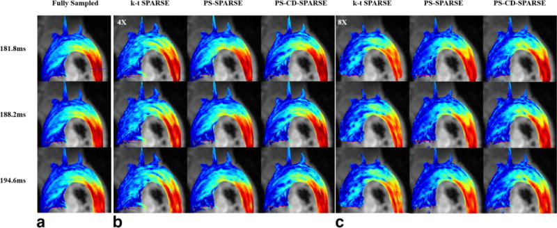
Pathline visualization using the particles released at three delay times (i.e., 181.8 ms, 188.2 ms, and 194.6 ms) after the R-wave. The pathlines obtained from the fully sampled flow data at the three time instants (a). The pathlines obtained from k-t SPARSE, PS-SPARSE, and PS-CD-SPARSE reconstructions at R = 4 (b) and R = 8 (c).

Figure 8 plots the time-resolved mean flow profiles for the cross-section plane through the AAo and DAo (as labeled in Figure 7). Compared with k-t SPARSE and PS-SPARSE, the proposed method yields more accurate flow profiles (e.g., less error in the peak velocity estimation). Note that the 3D experimental results are consistent with those from the 2D experiments. Additionally, the CD images reconstructed respectively by k-t SPARSE, PS-SPARSE and PS-CD-SPARSE at the acceleration factor R = 8 were also obtained. The reconstruction results from three slices are shown in Supporting Figure S1.

FIG. 8.

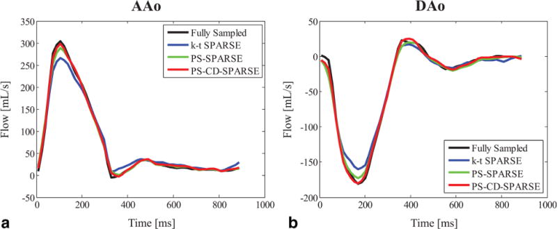
Flow profiles through the AAo (a) and DAo (b) obtained from k-t SPARSE, PS-SPARSE and PS-CD-SPARSE at R = 8 for the 3D retrospectively undersampled experiments.

Supporting Figure S2 shows the mean and standard deviation of the RMSE and error angles for the reconstructed velocities for all volunteers in the 3D retrospectively undersampled experiments. As can be seen, PS-CD-SPARSE yields higher accuracy than the other two methods. Additionally, we show the Bland-Altman plots of the peak velocities and stroke volumes for the fully sampled reference and the three reconstruction techniques with R = 8 in Supporting Figure S3. It can be clearly demonstrated that the peak velocity and stroke volume derived from proposed method show higher agreement with the fully sampled reference relative to the other two techniques.

Figure 9a shows the flow profiles associated with the proposed reconstruction at R = 8 for the 3D prospectively undersampled experiments. It can be seen that the proposed method captures the flow variation with good fidelity. Figure 9b shows the Bland-Altman analysis of the peak velocity and stroke volume for all volunteers. For the proposed method, the mean difference and standard deviation in peak velocity is 1.89 ± 1.28 cm/s, and in stroke volume is 0.66 ± 1.61 mL.

FIG. 9.

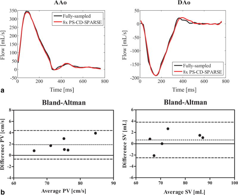
3D prospectively undersampled experiments. a: Flow profiles through the AAo and DAo obtained from the reference with fully sampled data and the proposed method with R = 8. b: Bland-Altman analysis of the peak velocity (PV) and stroke volume (SV) for the fully sampled reference and the proposed reconstruction with R = 8.

DISCUSSION

In this work, we have developed a new model-based reconstruction method and evaluated its performance with undersampled 2D and 3D in vivo PC-MRI of the aortic arch. For simplicity, here we integrated the variable-density sampling scheme with the prospective ECG triggering technique. Note that with such a triggering technique, the data acquisition typically does not cover the entire cardiac cycle, which may constrain the effectiveness of the proposed method for certain applications (e.g., studying early systolic flow). For these scenarios, it would be useful to incorporate the proposed method with the retrospective ECG gating. Systematically investigating and evaluating such an extension is beyond the scope of this work, but could enhance the practical utility of the proposed method for a wider range of applications.

In conventional 2D PC flow experiments, the slice is usually positioned perpendicular to the aorta, measuring the through-plane flow with only one FH-direction velocity encoding. However, considering the 2D sagittal plane with three-direction velocity encodings can be beneficial to the detection of abnormal flow variation for the patients with aortic dissection or aortic aneurysm, we chose to perform the 2D sagittal PC flow experiments with all the three-direction velocities analyzed at the same time. In addition, we evaluated the proposed method for the 2D axial PC flow imaging. Note that different from the previous ones, this new experiment can be accomplished within a single breath hold. We summarize the related reconstruction results and comparison in the supplementary material associated with this paper (shown in Supporting Figure S4). This set of new results further confirms the superior performance of the proposed method for accelerated PC flow MRI.

The proposed method needs to explicitly select a model order and a regularization parameter for image reconstruction. In this work, one set of parameters was selected to yield the minimum RMSE for one flow imaging dataset, and then we applied the same parameter values to other undersampled flow datasets acquired with the same imaging protocols. We have found that such an empirical way of selecting model parameters consistently yielded good reconstruction performance, although more principled approaches (34) can be investigated in the future study.

The computational efficiency of the proposed method depends on a number of factors, e.g., the number of measurements and receiver coils. For 2D PC-MRI, the proposed reconstruction is relatively efficient (e.g., it took around 16 min to perform reconstructions at R = 8 on a 64-bit windows PC with 32 GB of RAM). However, for 3D PC-MRI data, the proposed method is computationally more expensive (e.g., the runtime was more than 1h for the proposed reconstruction at R = 8). The GPU implementation of the proposed algorithm may be useful for computational acceleration, given the inherent algorithmic structure. However, note that the massive data resulting from 4D flow imaging can pose a significant challenge. To resolve this issue, sophisticated coordination between CPU and GPU needs to be carefully performed, which remains an interesting open question.

Joint low-rank and sparsity constraints based reconstruction has been applied to a variety of spatiotemporal imaging applications, including dynamic imaging (34,43,44), MR relaxometry (45), and MR spectroscopic imaging (46). Here we present the first investigation of these constraints with complex difference constraint for accelerated PC-MRI. Given that the complex difference constraint has previously been used with the sparsity to accelerate PC-MRI (38), we further performed a 2D in vivo PC-MRI experiment to compare the proposed method with such an approach (named as CS with CD). The reconstructed velocity maps and corresponding error maps obtained from the two methods are shown in Figure 10. Clearly, the proposed method produced more accurate velocity measurements at high acceleration factor, which further demonstrated the benefits of imposing the joint constraints.

FIG. 10.

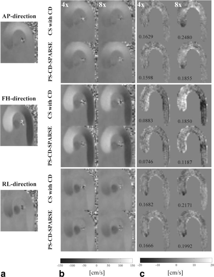
Reconstructed velocity maps for a systolic cardiac phase at two different acceleration factors. a: Reference from the fully sampled data along the AP, FH, and RL directions. b: The reconstructed velocity maps using the method from Ref. 38 and the proposed method at R = 4 and 8. c: The velocity error maps within the masked ROI. Note that the corresponding RMSE is labeled at the lower left corner of each error map.

A potential limitation of the proposed method is error propagation, given that the reconstruction accuracy of flow-reference images can affect subsequent reconstruction of flow-encoded images. To minimize such an effect, we have to obtain high quality reconstruction of flow-reference images. In this work, we manually optimized the rank and regularization parameters of the proposed method to ensure that error propagation was well controlled. In future research, it is worthwhile to study error propagation in a systematic way.

This work is focused on presenting a general image reconstruction method for PC-MRI. Although the proposed method enables improved accuracy over several state-of-the-art methods, its clinical utility has not been evaluated. We plan to conduct systematic clinical study of the proposed method (e.g., with respect to certain cardiovascular pathology) in a subsequent work.

CONCLUSIONS

In this work, we proposed a new model-based reconstruction method to accelerate PC-MRI, which consists of reconstruction of flow-reference image sequence and complex differences. Each problem was then effectively solved by incorporating the joint partial separability and sparsity constrained reconstruction with the ESPIRiT based parallel imaging model. Both 2D and 3D in vivo PC-MRI experiments were performed to evaluate the performance of the proposed method, and the results demonstrate that the proposed method enables more accurate velocity measurements and flow visualization with highly undersampled (k, -t)-space data, compared with several state-of-the-art reconstruction methods. The proposed method has demonstrated great potential to enhance the practical utility of PC-MRI.

Supplementary Material

Supplemental Material

Additional Supporting Information may be found in the online version of this article.

Table S1. Pearson’s correlation statistics between fully-sampled and reconstructed velocities from 2D retrospectively undersampled data for six volunteers.

Fig. S1. Magnitude of the reconstructed complex differences of three slices associated with a systolic cardiac phase from 3D retrospectively under-sampled data. a. Reference from the fully sampled data and the reconstructed complex differences using k-t SPARSE, PS-SPARSE and PS-CD-SPARSE at the acceleration factor R = 8. b: The error maps associated with the reconstructions in (a).

Fig. S2. 3D retrospectively undersampled experiments. a: Mean and standard deviation for the overall RMSE of the magnitudes of the reconstructed velocities. b: Mean and standard deviation for the angles between the reconstructed velocity vectors and those from the fully sampled data. Note that the above metrics were calculated with respect to the six volunteers and included all the pixels within the ROI.

Fig. S3. Bland-Altman plots of the peak velocities and stroke volumes derived from k-t SPARSE, PS-SPARSE and PS-CD-SPARSE respectively from 3D retrospectively undersampled data at R = 8.

Fig. S4. Reconstructed velocity maps for a systolic cardiac phase at different acceleration factors for 2D axial flow experiments. a: Reference from the fully sampled data along FH direction. b: The reconstructed velocity maps using k-t SPARSE, PS-SPARSE and PS-CD-SPARSE at R = 4 and 8. c: The associated velocity error maps for the reconstructions in (b) within the masked ROI. Note that the corresponding RMSE is labeled at the lower right corner of each error map.

APPENDIX

In this appendix, we describe the algorithms for solving Eqs. [3] and [4], which extend the half-quadratic regularization with continuation based algorithm in (34). To solve Eq. [3], we first convert it into the following half-quadratic regularization problem using variable splitting:

$$\underset{\left\{{\mathbf{U}}_{\mathrm{s}}^j,{\mathbf{G}}^j\right\}}{min}{\displaystyle \sum _{i=1}^{Nc}{\Vert {\mathbf{d}}_i-\mathrm{\Omega }[{\mathbf{F}}_{\mathrm{s}}{\displaystyle \sum _{j=1}^2{\mathbf{S}}_i^j({\mathbf{U}}_{\mathrm{s}}^j{\mathbf{V}}_t)]}\Vert }_2^2+\frac{\mathrm{\lambda }}{2\mathrm{\alpha }}}{\displaystyle \sum _{j=1}^2{\Vert {\mathbf{U}}_{\mathrm{s}}^j{\mathbf{V}}_{\mathrm{f}}-{\mathbf{G}}^j\Vert }_{\mathrm{F}}^2}+\mathrm{\lambda }{\displaystyle \sum _{j=1}^2{\Vert \text{vec}({\mathbf{G}}^j)\Vert }_1,}$$ [A1]

where G^j is an auxiliary matrix. Equation [A1] can then be solved by an alternating minimization with respect to ${\mathbf{U}}_{\mathrm{s}}^j$and G^j as follows:

$$<{\mathbf{G}}^{1(k+1)},{\mathbf{G}}^{2(k+1)}>=\arg \underset{{\mathbf{G}}^1\in {ℂ}^{N\times T},{\mathbf{G}}^2{\in }^{N\times T}}{min}\frac{1}{2\mathrm{\alpha }}{\displaystyle \sum _{j=1}^2{\Vert {\mathbf{U}}_{\mathrm{s}}^{j(k)}{\mathbf{V}}_{\mathrm{f}}-{\mathbf{G}}^j\Vert }_{\mathrm{F}}^2}+{\displaystyle \sum _{j=1}^2{\Vert \text{vec}({\mathbf{G}}^j)\Vert }_1,}$$ [A2]

$$<{\mathbf{U}}_{\mathrm{s}}^{1(k+1)},{\mathbf{U}}_{\mathrm{s}}^{2(k+1)}>=\arg \underset{{\mathbf{U}}_{\mathrm{s}}^1,{\mathbf{U}}_{\mathrm{s}}^2\in {ℂ}^{N\times L}}{min}{\displaystyle \sum _{i=1}^{Nc}{\Vert {\mathbf{d}}_i-\mathrm{\Omega }({\mathbf{F}}_{\mathrm{s}}{\displaystyle \sum _{j=1}^2{\mathbf{S}}_i^j({\mathbf{U}}_{\mathrm{s}}^j{\mathbf{V}}_{\mathrm{t}}))}\Vert }_2^2+\frac{\mathrm{\lambda }}{2\mathrm{\alpha }}{\displaystyle \sum _{j=1}^2{\Vert {\mathbf{U}}_{\mathrm{s}}^j{\mathbf{V}}_{\mathrm{f}}-{\mathbf{G}}^{j(k+1)}\Vert }_{\mathrm{F}}^2.}}$$ [A3]

The optimization problem in Eq. [A2] can be solved by the soft-thresholding operation, i.e.,

$${\mathbf{G}}^{j(k+1)}=S{({\mathbf{U}}_{\mathrm{s}}^{j(k)}{\mathbf{V}}_{\mathrm{f}})}_{n,m}=\{\begin{array}{ll}0,\hfill & \text{if}\left|{({\mathbf{U}}_{\mathrm{s}}^{j(k)}{\mathbf{V}}_{\mathrm{f}})}_{n,m}\right|<\mathrm{\alpha }\hfill \\ \frac{{({\mathbf{U}}_{\mathrm{s}}^{j(k)}{\mathbf{V}}_{\mathrm{f}})}_{n,m}}{\left|{({\mathbf{U}}_{\mathrm{s}}^{j(k)}{\mathbf{V}}_{\mathrm{f}})}_{n,m}\right|}(|{({\mathbf{U}}_{\mathrm{s}}^{j(k)}{\mathbf{V}}_{\mathrm{f}})}_{n,m}|-\text{α)}.\hfill & \text{if}\left|{({\mathbf{U}}_{\mathrm{s}}^{j(k)}{\mathbf{V}}_{\mathrm{f}})}_{n,m}\right|\ge \mathrm{\alpha }\hfill \end{array}$$ [A4]

Equation [A3] is a least-squares problem, whose solution can be obtained by solving

$$\left({\displaystyle \sum _{i=1}^{N_c}\left[\begin{array}{l}\begin{array}{l}{\mathbf{S}}_i^{1\ast }\hfill \\ {\mathbf{S}}_i^{2\ast }\hfill \end{array}\hfill \end{array}\right]{\mathbf{F}}_{\mathrm{s}}^{\ast }{\mathrm{\Omega }}^{\ast }\mathrm{\Omega }{\mathbf{F}}_s\left[\begin{array}{ll}{\mathbf{S}}_i^1\hfill & {\mathbf{S}}_i^2\hfill \end{array}\right]}+\frac{\mathrm{\lambda }}{2\mathrm{\alpha }}\mathbf{I}\right)\left[\begin{array}{l}{\mathbf{U}}_s^{1(k+1)}\hfill \\ {\mathbf{U}}_s^{2(k+1)}\hfill \end{array}\right]={\displaystyle \sum _{i=1}^{N_c}\left[\begin{array}{l}{\mathbf{S}}_i^{1\ast }\hfill \\ {\mathbf{S}}_i^{2\ast }\hfill \end{array}\right]}{\mathbf{F}}_{\mathrm{s}}^{\ast }{\mathrm{\Omega }}^{\ast }{\mathbf{d}}_i{\mathbf{V}}_{\mathrm{t}}^{\ast }+\frac{\mathrm{\lambda }}{2\mathrm{\alpha }}\left[\begin{array}{l}{\mathbf{G}}^{1(k+1)}\hfill \\ {\mathbf{G}}^{2(k+1)}\hfill \end{array}\right]{\mathbf{V}}_{\mathrm{f}}^{\ast }.$$ [A5]

In addition to the alternating minimization, a continuation procedure is applied by setting a initially large and gradually reducing it to zero, which ensures the solution of the half-quadratic optimization approaches that of the original optimization problem.

Regarding the optimization problem in Eq. [4], we first rewrite it as

$$<\Delta {\widehat{\mathbf{U}}}_{\mathrm{s}}^1,\Delta {\widehat{\mathbf{U}}}_{\mathrm{s}}^2>=\arg \underset{\Delta {\mathbf{U}}_{\mathrm{s}}^1,\Delta {\mathbf{U}}_{\mathrm{s}}^2\in {ℂ}^{N\times L}}{min}{\displaystyle \sum _{i=1}^{N_c}{\Vert \Delta {\mathbf{d}}_i-\mathrm{\Omega }\left[{\mathbf{F}}_s{\displaystyle \sum _{j=1}^2{\mathbf{S}}_i^j(\Delta {\mathbf{U}}_{\mathrm{s}}^j\Delta {\mathbf{V}}_{\mathrm{t}})}\right]\Vert }_2^2+\mathrm{\mu }{\displaystyle \sum _{j=1}^2\text{TV}(\Delta {\mathbf{U}}_s^j)=\arg \underset{\Delta {\mathbf{U}}_{\mathrm{s}}^1,\Delta {\mathbf{U}}_{\mathrm{s}}^2\in {ℂ}^{N\times L}}{min}{\displaystyle \sum _{i=1}^{N_c}{\Vert \Delta {\mathbf{d}}_i-\mathrm{\Omega }\left[{\mathbf{F}}_s{\displaystyle \sum _{j=1}^2{\mathbf{S}}_i^j(\Delta {\mathbf{U}}_{\mathrm{s}}^j\Delta {\mathbf{V}}_{\mathrm{t}})}\right]\Vert }_2^2+\mathrm{\mu }{{\displaystyle \sum _{j=1}^2{\displaystyle \sum _{l=1}^L{\displaystyle \sum _{n=1}^N\Vert \left[\begin{array}{l}{\mathbf{D}}_n^h\hfill \\ {\mathbf{D}}_n^v\hfill \end{array}\right]\Delta {\mathbf{U}}_s^{j(1)}\Vert }}}}_2,}}}$$ [A6]

where D^h; D^v ∈ ℂ ^{N × L} respectively denote the finite difference matrix associated with the horizontal and vertical directions, ${\mathbf{D}}_n^h$and ${\mathbf{D}}_n^v$ respectively denote the nth rows of D^h and D^v, and $\Delta {\mathbf{U}}_{\mathrm{s}}^{j(l)}$ denotes the 1th column of $\Delta {\mathbf{U}}_{\mathrm{s}}^j$. Note that Eq. [A6] can also be converted into a half-quadratic minimization problem as

$$\underset{\left\{\Delta {\mathbf{U}}_{\mathrm{s}}^j,{\mathbf{w}}_{nm}^j\right\}}{min}{{\displaystyle \sum _{i=1}^{N_c}\Vert {\mathbf{d}}_i-\mathrm{\Omega }\left[{\mathbf{F}}_s{\displaystyle \sum _{j=1}^2{\mathbf{S}}_i^j(\Delta {\mathbf{U}}_s^j\Delta {\mathbf{V}}_{\mathrm{t}})}\right]\Vert }}_2^2+\frac{\mathrm{\mu }}{2\mathrm{\alpha }}{\displaystyle \sum _{j=1}^2{\displaystyle \sum _{l=1}^L{\displaystyle \sum _{n=1}^N{\Vert {\mathbf{W}}_{nm}^j-\left[\begin{array}{l}{\mathbf{D}}_n^h\hfill \\ {\mathbf{D}}_n^v\hfill \end{array}\right]\Delta {\mathbf{U}}_{\mathrm{s}}^{j(l)}\Vert }_2^2+\mathrm{\mu }}}}{\displaystyle \sum _{j=1}^2{\displaystyle \sum _{l=1}^L{\displaystyle \sum _{n=1}^N{\Vert {\mathbf{w}}_{nm}^j\Vert }_2,}}}$$ [A7]

where ${\mathbf{w}}_{nm}^j$ is an auxiliary matrix. Again, the following alternation minimization is used to solve Eq. [A7]:

$${\mathbf{w}}_{nm}^{j(k+1)}=\arg \underset{{\mathbf{w}}_{nm}\in {ℂ}^2}{min}\frac{1}{2\mathrm{\alpha }}{\Vert {\mathbf{w}}_{nm}^j-\left[\begin{array}{l}{\mathbf{D}}_n^h\hfill \\ {\mathbf{D}}_n^v\hfill \end{array}\right]\Delta {\mathbf{U}}_s^{j(l)(k)}\Vert }_2^2+{\Vert {\mathbf{w}}_{nm}^j\Vert }_2,$$ [A8]

$$<\Delta {\widehat{\mathbf{U}}}_{\mathrm{s}}^{1(k+1)},\Delta {\widehat{\mathbf{U}}}_{\mathrm{s}}^{2(k+1)}>=\arg \underset{\Delta {\widehat{\mathbf{U}}}_{\mathrm{s}}^1,\Delta {\widehat{\mathbf{U}}}_{\mathrm{s}}^2\in {ℂ}^{N\times L}}{min}{\displaystyle \sum _{i=1}^{N_c}{\Vert {\mathbf{d}}_i-\mathrm{\Omega }\left[{\mathbf{F}}_{\mathrm{s}}{\displaystyle \sum _{j=1}^2{\mathrm{S}}_i^j(\Delta {\mathbf{U}}_{\mathrm{s}}^j\Delta {\mathbf{V}}_{\mathrm{t}}}\right]\Vert }_2^2+\frac{\mathrm{\mu }}{2\mathrm{\alpha }}{\displaystyle \sum _{j=1}^2{\displaystyle \sum _{l=1}^L{\displaystyle \sum _{n=1}^N{\Vert {\mathbf{w}}_{nm}^{j(k+1)}-\left[\begin{array}{l}{\mathbf{D}}_n^h\hfill \\ {\mathbf{D}}_n^v\hfill \end{array}\right]\Delta {\mathbf{U}}_s^{j(l)}\Vert }_2^2.}}}}$$ [A9]

To solve Eq. [A8], we use the two-dimensional soft-thresholding as follows:

$${\mathbf{w}}_{nm}^{j(k+1)}=\frac{\left[\begin{array}{l}{\mathbf{D}}_n^h\hfill \\ {\mathbf{D}}_n^v\hfill \end{array}\right]\Delta {\mathbf{U}}_s^{j(l)(k)}}{{\Vert \left[\begin{array}{l}{\mathbf{D}}_n^h\hfill \\ {\mathbf{D}}_n^v\hfill \end{array}\right]\Delta {\mathbf{U}}_s^{j(l)(k)}\Vert }_2}max\left\{{\Vert \left[\begin{array}{l}{\mathbf{D}}_n^h\hfill \\ {\mathbf{D}}_n^v\hfill \end{array}\right]\Delta {\mathbf{U}}_s^{j(l)(k)}\Vert }_2-\mathrm{\alpha },0\right\}.$$ [A10]

For Eq. [A9], it can be determined by solving the following normal equations:

$$\left({\displaystyle \sum _{i=1}^{N_c}\left[\begin{array}{l}{\mathbf{S}}_i^{1\ast }\hfill \\ {\mathbf{S}}_i^{2\ast }\hfill \end{array}\right]{\mathbf{F}}_{\mathrm{s}}^{\ast }{\mathrm{\Omega }}^{\ast }\Omega {\mathbf{F}}_{\mathrm{s}}\left[\begin{array}{ll}{\mathbf{s}}_i^1\hfill & {\mathbf{s}}_i^2\hfill \end{array}\right]+\frac{\mathrm{\mu }}{2\mathrm{\alpha }}}{\left({\mathbf{D}}^h\right)}^{\ast }{\mathbf{D}}^h+\frac{\mathrm{\mu }}{2\mathrm{\alpha }}{\left({\mathbf{D}}^v\right)}^{\ast }{\mathbf{D}}^v\right)\left[\begin{array}{l}\Delta {\mathbf{U}}_{\mathrm{s}}^{1(k+1)}\hfill \\ \Delta {\mathbf{U}}_{\mathrm{s}}^{2(k+1)}\hfill \end{array}\right]={\displaystyle \sum _{i=1}^{N_c}\left[\begin{array}{l}{\mathbf{S}}_i^{1\ast }\hfill \\ {\mathbf{S}}_i^{2\ast }\hfill \end{array}\right]{\mathbf{F}}_{\mathrm{s}}^{\ast }{\mathrm{\Omega }}^{\ast }{\mathbf{d}}_i{\mathbf{V}}_t^{\ast }+}\frac{\mathrm{\mu }}{2\mathrm{\alpha }}{\left({\mathbf{D}}^h\right)}^{\ast }\left[\begin{array}{l}{\mathbf{w}}^{1,h(k+1)}\hfill \\ {\mathbf{w}}^{2,h(k+1)}\hfill \end{array}\right]+\frac{\mathrm{\mu }}{2\mathrm{\alpha }}{\left({\mathbf{D}}^v\right)}^{\ast }\left[\begin{array}{l}{\mathbf{w}}^{1,v(k+1)}\hfill \\ {\mathbf{w}}^{2,v(k+1)}\hfill \end{array}\right].$$ [A11]

We apply a similar continuation procedure on a to obtain the solution to the original optimization problem in Eq. [4].

References

- 1.Bryant D, Payne J, Firmin D, Longmore D. Measurement of flow with NMR imaging using a gradient pulse and phase difference technique. J Comput Assist Tomogr. 1984;8:588–593. doi: 10.1097/00004728-198408000-00002. [DOI] [PubMed] [Google Scholar]
- 2.Nayler G, Firmin D, Longmore D. Blood flow imaging by cine magnetic resonance. J Comput Assist Tomogr. 1986;10:715–722. doi: 10.1097/00004728-198609000-00001. [DOI] [PubMed] [Google Scholar]
- 3.Axel L, Morton D. MR flow imaging by velocity-compensated/uncompensated difference images. J Comput Assist Tomogr. 1987;11:31–34. doi: 10.1097/00004728-198701000-00006. [DOI] [PubMed] [Google Scholar]
- 4.Markl M, Frydrychowicz A, Kozerke S, Hope M, Wieben O. 4D flow MRI. J Magn Reson Imaging. 2012;36:1015–1036. doi: 10.1002/jmri.23632. [DOI] [PubMed] [Google Scholar]
- 5.Markl M, Kilner PJ, Ebbers T. Comprehensive 4D velocity mapping of the heart and great vessels by cardiovascular magnetic resonance. J Cardiovasc Magn Reson. 2011;13:1–22. doi: 10.1186/1532-429X-13-7. [DOI] [PMC free article] [PubMed] [Google Scholar]
- 6.Osinnski JN, Ku DN, Mukundan S, Loth F, Pettigrew RI. Determination of wall shear stress in the aorta with the use of MR phase velocity mapping. J Magn Reson Imaging. 1995;5:640–647. doi: 10.1002/jmri.1880050605. [DOI] [PubMed] [Google Scholar]
- 7.Oyre S, Paaske W, Ringgaard S, Kozerke S, Erlandsen M, Boesiger P, Pedersen EM. Automatic accurate non-invasive quantitation of blood flow, cross-sectional vessel area, and wall shear stress by modelling of magnetic resonance velocity data. Eur J Vasc Endovasc Surg. 1998;16:517–524. doi: 10.1016/s1078-5884(98)80244-x. [DOI] [PubMed] [Google Scholar]
- 8.Frydrychowicz A, Stalder AF, Russe MF, Bock J, Bauer S, Harloff A, Berger A, Langer M, Hennig J, Markl M. Three-dimensional analysis of segmental wall shear stress in the aorta by flow-sensitive four-dimensional-MRI. J Magn Reson Imaging. 2009;30:77–84. doi: 10.1002/jmri.21790. [DOI] [PubMed] [Google Scholar]
- 9.Tyszka JM, Laidlaw DH, Asa JW, Silverman JM. Three-dimensional, time-resolved (4D) relative pressure mapping using magnetic resonance imaging. J Magn Reson Imaging. 2000;12:321–329. doi: 10.1002/1522-2586(200008)12:2<321::aid-jmri15>3.0.co;2-2. [DOI] [PubMed] [Google Scholar]
- 10.Ebbers T, Wigstrom L, Bolger A, Wranne B, Karlsson M. Noninvasive measurement of time-varying three-dimensional relative pressure fields within the human heart. J Biomech Eng. 2002;124:288–293. doi: 10.1115/1.1468866. [DOI] [PubMed] [Google Scholar]
- 11.Bock J, Frydrychowicz A, Lorenz R, Hirtler D, Barker AJ, Johnson KM, Arnold R, Burkhardt H, Hennig J, Markl M. In vivo noninvasive 4D pressure difference mapping in the human aorta: phantom comparison and application in healthy volunteers and patients. Magn Reson Med. 2011;66:1079–1088. doi: 10.1002/mrm.22907. [DOI] [PubMed] [Google Scholar]
- 12.Bolster BD, Atalar E, Hardy CJ, McVeigh ER. Accuracy of arterial pulse-wave velocity measurement using MR. J Magn Reson Imaging. 1998;8:878–888. doi: 10.1002/jmri.1880080418. [DOI] [PMC free article] [PubMed] [Google Scholar]
- 13.Markl M, Wallis W, Brendecke S, Simon J, Frydrychowicz A, Harloff A. Estimation of global aortic pulse wave velocity by flow-sensitive 4D MRI. Magn Reson Med. 2010;63:1575–1582. doi: 10.1002/mrm.22353. [DOI] [PubMed] [Google Scholar]
- 14.Hope TA, Markl M, Wigström L, Alley MT, Miller DC, Herfkens RJ. Comparison of flow patterns in ascending aortic aneurysms and volunteers using four-dimensional magnetic resonance velocity mapping. J Magn Reson Imaging. 2007;26:1471–1479. doi: 10.1002/jmri.21082. [DOI] [PubMed] [Google Scholar]
- 15.Hope TA, Hope MD, Purcell DD, von Morze C, Vigneron DB, Alley MT, Dillon WP. Evaluation of intracranial stenoses and aneurysms with accelerated 4D flow. Magn Reson Imaging. 2010;28:41–46. doi: 10.1016/j.mri.2009.05.042. [DOI] [PubMed] [Google Scholar]
- 16.Ansari S, Schnell S, Carroll T, Vakil P, Hurley M, Wu C, Carr J, Bendok B, Batjer H, Markl M. Intracranial 4D flow MRI: toward individualized assessment of arteriovenous malformation hemodynamics and treatment-induced changes. Am J Neuroradiol. 2013;34:1922–1928. doi: 10.3174/ajnr.A3537. [DOI] [PMC free article] [PubMed] [Google Scholar]
- 17.Gu T, Korosec FR, Block WF, Fain SB, Turk Q, Lum D, Zhou Y, Grist TM, Haughton V, Mistretta CA. PC VIPR: a high-speed 3D phase-contrast method for flow quantification and high-resolution angiography. Am J Neuroradiol. 2005;26:743–749. [PMC free article] [PubMed] [Google Scholar]
- 18.Pike GB, Meyer CH, Brosnan TJ, Pelc NJ. Magnetic resonance velocity imaging using a fast spiral phase contrast sequence. Magn Reson Med. 1994;32:476–483. doi: 10.1002/mrm.1910320409. [DOI] [PubMed] [Google Scholar]
- 19.Sigfridsson A, Petersson S, Carlhäll CJ, Ebbers T. Four-dimensional flow MRI using spiral acquisition. Magn Reson Med. 2012;68:1065–1073. doi: 10.1002/mrm.23297. [DOI] [PubMed] [Google Scholar]
- 20.Pruessmann KP, Weiger M, Scheidegger MB, Boesiger P. SENSE: sensitivity encoding for fast MRI. Magn Reson Med. 1999;42:952–962. [PubMed] [Google Scholar]
- 21.Griswold MA, Jakob PM, Heidemann RM, Nittka M, Jellus V, Wang J, Kiefer B, Haase A. Generalized autocalibrating partially parallel acquisitions (GRAPPA) Magn Reson Med. 2002;47:1202–1210. doi: 10.1002/mrm.10171. [DOI] [PubMed] [Google Scholar]
- 22.Tsao J, Boesiger P, Pruessmann KP. k-t BLAST and k-t SENSE: dynamic MRI with high frame rate exploiting spatiotemporal correlations. Magn Reson Med. 2003;50:1031–1042. doi: 10.1002/mrm.10611. [DOI] [PubMed] [Google Scholar]
- 23.Baltes C, Kozerke S, Hansen MS, Pruessmann KP, Tsao J, Boesiger P. Accelerating cine phase-contrast flow measurements using k-t BLAST and k-t SENSE. Magn Reson Med. 2005;54:1430–1438. doi: 10.1002/mrm.20730. [DOI] [PubMed] [Google Scholar]
- 24.Huang F, Akao J, Vijayakumar S, Duensing GR, Limkeman M. k-t GRAPPA: a k-space implementation for dynamic MRI with high reduction factor. Magn Reson Med. 2005;54:1172–1184. doi: 10.1002/mrm.20641. [DOI] [PubMed] [Google Scholar]
- 25.Jung B, Stalder AF, Bauer S, Markl M. On the undersampling strategies to accelerate time-resolved 3D imaging using k-t-GRAPPA. Magn Reson Med. 2011;66:966–975. doi: 10.1002/mrm.22875. [DOI] [PubMed] [Google Scholar]
- 26.Santelli C, Schaeffter T, Kozerke S. Radial k-t SPIRiT: autocalibrated parallel imaging for generalized phase-contrast MRI. Magn Reson Med. 2014;72:1233–1245. doi: 10.1002/mrm.25030. [DOI] [PubMed] [Google Scholar]
- 27.Lustig M, Donoho D, Pauly JM. Sparse MRI: the application of compressed sensing for rapid MR imaging. Magn Reson Med. 2007;58:1182–1195. doi: 10.1002/mrm.21391. [DOI] [PubMed] [Google Scholar]
- 28.Jung H, Sung K, Nayak KS, Kim EY, Ye JC. k-t FOCUSS: a general compressed sensing framework for high resolution dynamic MRI. Magn Reson Med. 2009;61:103–116. doi: 10.1002/mrm.21757. [DOI] [PubMed] [Google Scholar]
- 29.Liang ZP. Spatiotemporal imaging with partially separable functions. Proceedings of IEEE International Symposium on Biomedical Imaging; Washington, DC, USA. 2007. pp. 988–991. [Google Scholar]
- 30.Pedersen H, Kozerke S, Ringgaard S, Nehrke K, Kim WY. k-t PCA: temporally constrained k-t BLAST reconstruction using principal component analysis. Magn Reson Med. 2009;62:706–716. doi: 10.1002/mrm.22052. [DOI] [PubMed] [Google Scholar]
- 31.Zhao B, Haldar JP, Brinegar C, Liang ZP. Low rank matrix recovery for real-time cardiac MRI. Proceedings of IEEE International Symposium on Biomedical Imaging; Rotterdam, The Netherlands. 2010. pp. 996–999. [Google Scholar]
- 32.Haldar JP, Liang ZP. Spatiotemporal imaging with partially separable functions: a matrix recovery approach. Proceedings of IEEE International Symposium on Biomedical Imaging; Rotterdam, The Netherlands. 2010. pp. 716–719. [Google Scholar]
- 33.Lingala SG, Hu Y, DiBella E, Jacob M. Accelerated dynamic MRI exploiting sparsity and low-rank structure: k-t SLR. IEEE Trans Med Imaging. 2011;30:1042–1054. doi: 10.1109/TMI.2010.2100850. [DOI] [PMC free article] [PubMed] [Google Scholar]
- 34.Zhao B, Haldar JP, Christodoulou AG, Liang ZP. Image reconstruction from highly undersampled (k, t)-space data with joint partial separability and sparsity constraints. IEEE Trans Med Imaging. 2012;31:1809–1820. doi: 10.1109/TMI.2012.2203921. [DOI] [PMC free article] [PubMed] [Google Scholar]
- 35.Giese D, Schaeffter T, Kozerke S. Highly undersampled phase-contrast flow measurements using compartment-based k-t principal component analysis. Magn Reson Med. 2013;69:434–443. doi: 10.1002/mrm.24273. [DOI] [PubMed] [Google Scholar]
- 36.Knobloch V, Boesiger P, Kozerke S. Sparsity transform k-t principal component analysis for accelerating cine three-dimensional flow measurements. Magn Reson Med. 2013;70:53–63. doi: 10.1002/mrm.24431. [DOI] [PubMed] [Google Scholar]
- 37.Kim D, Dyvorne HA, Otazo R, Feng L, Sodickson DK, Lee VS. Accelerated phase-contrast cine MRI using k-t SPARSE-SENSE. Magn Reson Med. 2012;67:1054–1064. doi: 10.1002/mrm.23088. [DOI] [PMC free article] [PubMed] [Google Scholar]
- 38.Kwak Y, Nam S, Akçakaya M, Basha TA, Goddu B, Manning WJ, Tarokh V, Nezafat R. Accelerated aortic flow assessment with compressed sensing with and without use of the sparsity of the complex difference image. Magn Reson Med. 2013;70:851–858. doi: 10.1002/mrm.24514. [DOI] [PMC free article] [PubMed] [Google Scholar]
- 39.Zhao B, Sun A, Ma K, Li R, Christodoulou A, Yuan C, Liang ZP. Real-time phase contrast cardiovascular flow imaging with joint low-rank and sparsity constraints. Proceedings of the 23rd Annual Meeting of ISMRM; Milan, Italy: 2014. p. 743. [Google Scholar]
- 40.Uecker M, Lai P, Murphy MJ, Virtue P, Elad M, Pauly JM, Vasanawala SS, Lustig M. ESPIRiT-an eigenvalue approach to autocalibrating parallel MRI: where SENSE meets GRAPPA. Magn Reson Med. 2014;71:990–1001. doi: 10.1002/mrm.24751. [DOI] [PMC free article] [PubMed] [Google Scholar]
- 41.Zhao B, Haldar JP, Christodoulou AG, Liang ZP. Further development of image reconstruction from highly undersampled (k, t)-space data with joint partial separability and sparsity constraints. Proceedings of IEEE International Symposium on Biomedical Imaging; Chicago, Illinois, USA. 2011. pp. 1593–1596. [Google Scholar]
- 42.Walker PG, Cranney GB, Scheidegger MB, Waseleski G, Pohost GM, Yoganathan AP. Semiautomated method for noise reduction and background phase error correction in MR phase velocity data. J Magn Reson Imaging. 1993;3:521–530. doi: 10.1002/jmri.1880030315. [DOI] [PubMed] [Google Scholar]
- 43.Christodoulou AG, Zhang H, Zhao B, Hitchens TK, Ho C, Liang ZP. High-resolution cardiovascular MRI by integrating parallel imaging with low-rank and sparse modeling. IEEE Trans Biomed Eng. 2013;60:3083–3092. doi: 10.1109/TBME.2013.2266096. [DOI] [PMC free article] [PubMed] [Google Scholar]
- 44.Fu M, Zhao B, Carignan C, Shosted RK, Perry JL, Kuehn DP, Liang ZP, Sutton BP. High-resolution dynamic speech imaging with joint low-rank and sparsity constraints. Magn Reson Med. 2015;73:1820–1832. doi: 10.1002/mrm.25302. [DOI] [PMC free article] [PubMed] [Google Scholar]
- 45.Zhao B, Lu W, Hitchens TK, Lam F, Ho C, Liang ZP. Accelerated MR parameter mapping with low-rank and sparsity constraints. Magn Reson Med. 2015;74:489–498. doi: 10.1002/mrm.25421. [DOI] [PMC free article] [PubMed] [Google Scholar]
- 46.Lam F, Liang ZP. A subspace approach to high-resolution spectroscopic imaging. Magn Reson Med. 2014;71:1349–1357. doi: 10.1002/mrm.25168. [DOI] [PMC free article] [PubMed] [Google Scholar]
Associated Data
This section collects any data citations, data availability statements, or supplementary materials included in this article.
Supplementary Materials