Comparison of region-of-interest-averaged and pixel-averaged analysis of DCE-MRI data based on simulations and pre-clinical experiments

Abstract

Differences between region-of-interest (ROI) and pixel-by-pixel analysis of dynamic contrast enhanced (DCE) MRI data were investigated in this study with computer simulations and pre-clinical experiments. ROIs were simulated with 10, 50, 100, 200, 400, and 800 different pixels. For each pixel, a contrast agent concentration as a function of time, C(t), was calculated using the Tofts DCE-MRI model with randomly generated physiological parameters (K^trans and v_e) and the Parker population arterial input function. The average C(t) for each ROI was calculated and then K^trans and v_e for the ROI was extracted. The simulations were run 100 times for each ROI with new K^trans and v_e generated. In addition, white Gaussian noise was added to C(t) with 3, 6, and 12 dB signal-to-noise ratios to each C(t). For pre-clinical experiments, Copenhagen rats (n = 6) with implanted prostate tumors in the hind limb were used in this study. The DCE-MRI data were acquired with a temporal resolution of ~5 s in a 4.7 T animal scanner, before, during, and after a bolus injection (< 5 s) of Gd-DTPA for a total imaging duration of ~10 min. K^trans and v_e were calculated in two ways: (i) by fitting C(t) for each pixel, and then averaging the pixel values over the entire ROI, and (ii) by averaging C(t) over the entire ROI, and then fitting C(t) to extract K^trans and v_e. The simulation results showed that in heterogeneous ROIs, the pixel-by-pixel averaged K^trans was ~25% to ~50% larger (p < 0.01) than the ROI-averaged K^trans. At higher noise levels, the pixel-averaged K^trans was greater than the ‘true’ K^trans, but the ROI-averaged K^trans was lower than the ‘true’ K^trans. The ROI-averaged K^trans was closer to the true K^trans than pixel-averaged K^trans for high noise levels. In pre-clinical experiments, the pixel-by-pixel averaged K^trans was ~15% larger than the ROI-averaged K^trans. Overall, with the Tofts model, the extracted physiological parameters from the pixel-by-pixel averages were larger than the ROI averages. These differences were dependent on the heterogeneity of the ROI.

1. Introduction

Dynamic contrast enhanced MRI (DCE-MRI) plays an important role in clinical detection and diagnosis of cancers (Engelbrecht et al., 2003, Franiel et al., 2011, Mehrabian et al., 2015), and in evaluating response to therapy (Leach et al., 2012, O’Connor et al., 2012, Hotker et al., 2015). For quantitative analysis of DCE-MRI, the pharmacokinetic models, such as Tofts and extended Tofts models are often used to characterize the redistribution of contrast agent following a bolus injection (Tofts et al., 1999). The DCE-MRI data are frequently analyzed based on a region of interest (ROI) defined by a radiologist (Othman et al., 2016). For a specific ROI, normally the average contrast agent concentration curve as function of time over whole ROI is calculated first, and then the pharmacokinetic model is used to extract physiological parameters for the ROI (Langer et al., 2009, Hectors et al., 2017). We would like to call this as ‘ROI-averaged’ analysis. The ‘ROI-averaged’ analysis does not take into account the spatially heterogeneous enhancement within the ROI. In contrast to ‘ROI-averaged’ analysis, the physiological parameters for each pixel within the ROI can be extracted first, and then the averaged physiological parameters can be calculated from all the pixels within the ROI (Guo and Reddick, 2009, Lavini et al., 2009, Haney et al., 2013, Ng et al., 2015). We would like to call this a ‘pixel-averaged’ analysis. Although the pixel-averaged analysis is sensitive to the heterogeneity of perfusion within the ROI (Haney et al., 2013, Tokuda et al., 2011), the accuracy of fitting the pixel based contrast agent concentration curves could be severely affected by low signal to noise ratio (SNR). Nevertheless, both types of analysis are often used in DCE-MRI to extract physiological parameters and can both give suboptimal results.

While the effects of a heterogeneous ROI on physiological parameters extracted from the Tofts model are generally recognized and an effect of the non-linearity of the model can be anticipated (Guo and Reddick, 2009, Haney et al., 2013, Ng et al., 2015), the magnitude of those effects has not been studied systematically. Based on the Tofts model (Tofts et al., 1999), the change in contrast agent concentration as a function of time (C(t)) following contrast agent bolus injection is given by:

$$C\left(t\right)=K^{\text{trans}}{\displaystyle {\int }_0^t{C}_{\mathrm{p}}\left(\tau \right)\text{exp}\left(-\left(t-\tau \right)K^{\text{trans}}/v_e\right)d\tau ,}$$ (1)

where ‘t’ is time, C_p(t) is the arterial input function (AIF), K^trans is the volume transfer constant between blood plasma and extravascular extracellular space (EES), and v_e is the volume of EES per unit volume of tissue. To consider a simple example, we assume that an ROI has only two different contrast agent concentration curves, C_n(t) (n = 1, 2), that both satisfy the Eq. (1) with different values of K_n^trans and v_eⁿ. Then an average of the two curves (C_ave(t)) for the entire ROI may not satisfy the Tofts model, i.e.,

$$C_{\text{ave}}\left(t\right)=\frac{1}{2}\left(C_1\left(t\right)+C_2\left(t\right)\right)=\frac{1}{2}{\displaystyle {\int }_0^t{C}_{\mathrm{p}}\left(\tau \right)\left[K_1{ }^{\text{trans}}\text{exp}\left(-\left(t-\tau \right)K_1{ }^{\text{trans}}/v_e^1\right)+K_2{ }^{\text{trans}}\text{exp}\left(-\left(t-\tau \right)K_2{ }^{\text{trans}}/v_e^2\right)\right]}d\tau ,$$ (2)

because the above expression cannot be combined into a single term as in the Eq. (1) unless the ratio of K^trans/v_e is the same for each pixel. If the ratio of K^trans/v_e is the same for two pixels within the ROI, i.e., $K_1^{\mathit{trans}}/v_e^1=K_2^{\mathit{trans}}/v_e^2=k_{ep}$, then averaged K^trans and v_e is given by $K_{\mathit{ave}}^{\mathit{trans}}=\left(K_1^{\mathit{trans}}+K_2^{\mathit{trans}}\right)/2$ and $v_e^{\mathit{ave}}=K_{\mathit{ave}}^{\mathit{trans}}/k_{ep}$, respectively. However, in reality the ratio of K^trans/v_e in each pixel is likely to vary significantly within a tumor ROI. Therefore, the effects of non-linearity of Tofts model on extracted physiological parameters may be significant and should be investigated for heterogeneous ROIs in tumors.

In this study, computer simulations and DCE-MRI data from transplanted rodent prostate cancers were used to evaluate the differences in extracted physiological parameters from ‘ROI-averaged’ analysis versus ‘pixel-averaged’ analysis, with use of the Tofts model for analysis of heterogeneous ROIs.

2. Methods

2.1. Simulations for noise free curves

To study the effects of nonlinearity of the Tofts model, the random number generator in Matlab (version R2012b, MathWorks, Natick, MA, USA) was used to generate K^trans and v_e for each pixel within an ROI first, and then used to calculate the contrast agent concentration curve as function of time for the pixel (C(t)_pixel) by using the Eq. (1). The population AIF (C_p) developed by Parker et al. (Parker et al., 2006) was used in these calculations. The following steps were used in the computer simulations:

1. Temporal resolution of 5 seconds was used in the calculations, and the contrast agent concentration curves C(t) were sampled for 10 min.

2. Random numbers (r_n1 and r_n2) uniformly distributed between 0 and 1 were generated and mapped into the following interval to obtain practical K^trans and v_e values (Alonzi et al., 2010, Ocak et al., 2007):

   $$K^{\mathit{trans}}=0.05+r_{n1}\cdot \left(1.0-0.05\right)\text{and}{v}_e=0.05+r_{n2}\cdot \left(0.75-0.05\right).$$ (3)

   The randomly generated K^trans and v_e could not simply be combined because the ratio of K^trans/v_e also needs to be in a reasonable range. Based on previous studies (Chen et al., 2012, Li et al., 2016), only the values of K^trans and v_e such that K^trans/v_e< 10 were used in the calculations.

3. A total of six different sizes of ROIs were simulated with 10, 50, 100, 200, 400, and 800 pixels. For each pixel, C(t)_pixel was calculated by using Eq. (1) with randomly generated K^trans and v_e in step (ii). For each ROI, the simulations were run 100 times with new K^trans and v_e generated in step (ii).

4. The ‘pixel-averaged’ analysis was performed by calculating the average of the per-pixel K^trans and v_e used in step (ii) over the ROI. We refer to these averaged physiological parameters as K^trans(Pixel) and v_e(Pixel).

5. The ‘ROI-averaged’ analysis was performed by calculating the mean contrast agent concentration curve (C(t)_ROI = average of all C(t)_pixel) over the ROI, and then fitting C(t)_ROI to Eq. (1) to extract K^trans and v_e. We refer to these physiological parameters as K^trans(ROI) and v_e(ROI).

2.2. Simulations for noise curves

White Gaussian noise is often used in simulation studies to investigate noise effects. For example, Ahearn et al. (Ahearn et al., 2005) selected Gaussian noise to add to each C(t) curve using ten different standard deviations increasing from 0.0 to 0.9, which was equivalent to SNR of about 20 to 1 dB. In this study, the contrast agent concentration curve with noise $\left(\stackrel{\sim }{C}\left(t\right)\right)$ was generated by adding white Gaussian noise (n(t)) to each C(t)_pixel in the step (iii) above, as follows:

$$\stackrel{\sim }{C}{\left(t\right)}_{\text{pixel}}=C{\left(t\right)}_{\text{pixel}}+n\left(t\right).$$ (4)

Based on the previous study (Ahearn et al., 2005) and our pre-clinical experiments, three different levels of Gaussian noise with SNR values of 3, 6, and 12 dB, representing high, medium, and low noise levels encountered in real DCE-MRI experiments, were used in the simulations. Each $\left(\stackrel{\sim }{C}\left(t\right)\right)$ with added noise was refitted to Eq. (1) to extract new K^trans and v_e, which could be different from the original randomly generated values. Then steps (iv) and (v) were repeated for ‘pixel-averaged’ and ‘ROI-averaged’ analysis to study the effects of adding noise.

2.3. Animal experiments

MRI data were acquired on a 4.7 T (Bruker, Ettlingen, Germany) pre-clinical scanner at the University of Chicago, and all the procedures were carried out in accordance with the institution’s Animal Care and Use Committee approval. The Copenhagen rats (n = 6) used in this study were implanted in the hind limb with the prostate cell line AT2.1. The animals were anesthetized with isoflurane gas and oxygen during the whole imaging procedure at a rate of 1 – 2%. Heart rate, respiration rate, and temperature were continuously monitored using an SA instrument (Stony Brook, NY, USA) monitoring system during MRI experiments. Temperature was maintained using a warm air blower at 37 – 38 °C.

After T2-weighted (T2W) spin echo images and T1 maps were acquired, three slices of DCE T1-weighted gradient echo images (TR/TE = 40/3.5 ms, matrix size = 128×128, field of view = 40 mm, flip angle = 30°, slice thickness = 1 mm, gap = 0 mm) were acquired through the center of the tumor along the long axis of the leg with a temporal resolution of 5.12 s. A bolus (< 5 s) injection of contrast agent gadodiamide (Omniscan, GE Healthcare, Piscataway, NJ, USA) was given at a dose of 0.2 mmol/kg at ~30 s after DCE imaging was started. DCE-MRI data was continuously acquired for total ~10 min post-injection.

MRI data analysis was performed using Matlab with in-house software. For each pixel, the contrast agent concentration curve as function of time (C(t)) was calculated using a previously published method (Dale et al., 2003). The AIF was derived by using the reference tissue method based on a muscle ROI (41×5 pixels) in the center slice with literature values of K^trans (0.11 min⁻¹) and v_e (0.20) for rat muscle (Heisen et al., 2010). For each pixel, C(t) was fitted with Eq. (1) to extract the K^trans and v_e. The whole tumor ROI was manually traced on the T2W image and superimposed on the DCE-MRI data. The tumor was automatically segmented into the rim and the core. The tumor rim was defined as a two pixel thick ring along the tumor boundary, and all other tumor pixels were considered to be the core. The ‘pixel-averaged’ and ‘ROI-averaged’ analysis were performed for all these ROIs.

2.4. Statistical analysis

For each ROI with 100 simulations, One-way ANOVA and Tukey’s HSD (honestly significant difference) tests were performed to determine whether there was a significant difference for the physiological parameters obtained from ‘pixel-averaged’ analysis and ‘ROI-averaged’ analysis for the curves with and without adding noise. The Pearson correlation test was performed to examine whether there was a linear relationship between ‘pixel-averaged’ and ‘ROI-averaged’ analysis for K^trans and v_e. A p-value less than 0.05 was considered significant.

3. Results

3.1. Simulations

Figure 1 shows scatter plots of K^trans(Pixel) vs. K^trans(ROI) obtained from 100 simulations with (red solid squares) and without (black solid circles) noise (SNR = 3 dB) for the ROIs containing: (a) 10, (b) 50, (c) 100, (d) 200, (e) 400, and (f) 800 different pixels. The scattered K^trans values obtained with noise were shifted further away from the identity line (gray line) than the K^trans values without the noise. Over 100 simulations, larger ROI’s produced smaller coefficients of variation for K^trans. For each simulated ROI’s, one-way ANOVA and Tukey’s HSD showed that on average K^trans(Pixel) was ~50% and ~25% larger (p < 0.01) than K^trans(ROI) obtained with and without noise, respectively. Although the K^trans(ROI) was not greatly affected by noise, the K^trans(Pixel) with noise was ~20% larger than those values determined without noise, and this difference was highly significant (p < 0.01).

Figure 1.

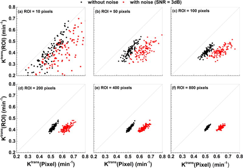
Scatter plots of K^trans(Pixel) vs. K^trans(ROI) obtained from 100 simulations with (red solid squares) and without (black solid circles) noise (SNR = 3 dB) added to C(t) for six different sizes of ROIs. The gray line is the line of equality. The sizes of ROIs were (a) 10, (b) 50, (c) 100, (d) 200, (e) 400, and (f) 800 pixels.

Similarly, Figure 2 shows scatter plots of v_e(Pixel) vs. v_e(ROI) obtained from 100 simulations with (red solid squares) and without (black solid circles) noise (SNR = 3 dB) for the ROIs containing: (a) 10, (b) 50, (c) 100, (d) 200, (e) 400, and (f) 800 different pixels. In contrast to K^trans, the v_e values are not significantly affected by noise. On average v_e(Pixel) was only slightly larger (~6%) than v_e(ROI) but this difference was not statistically significant, except for the ROI with 10 pixels.

Figure 2.

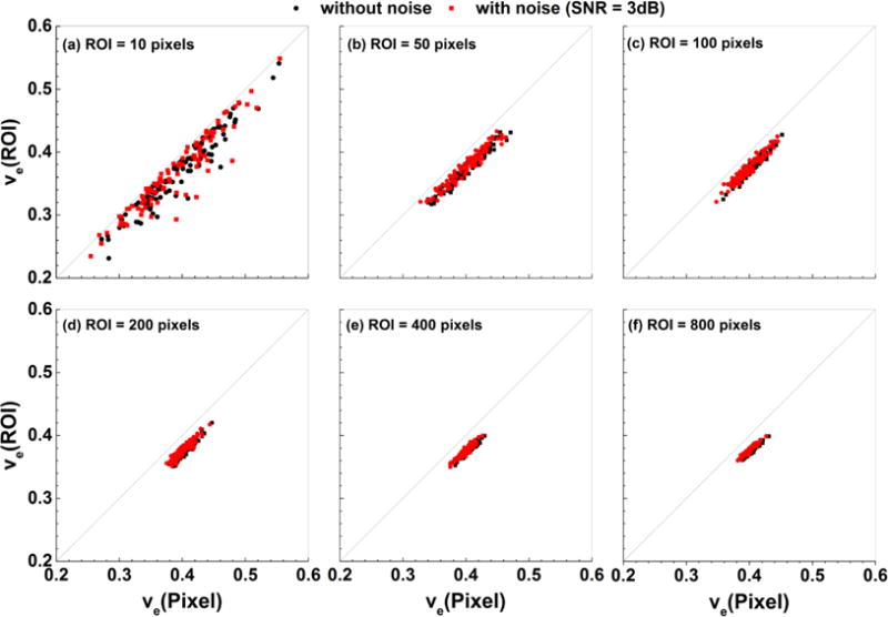
Scatter plots v_e(Pixel) vs. v_e(ROI) obtained from 100 simulations with (red solid squares) and without (black solid circles) noise (SNR = 3 dB) added to C(t) for six different sizes of ROIs. The gray line is the line of equality. The sizes of ROIs were (a) 10, (b) 50, (c) 100, (d) 200, (e) 400, and (f) 800 pixels.

The Pearson correlation tests showed that there were moderate to strong positive correlations (r > 0.60, p < 0.001) between K^trans(Pixel) vs. K^trans(ROI), and very strong positive correlations (r > 0.90, p < 0.001) between v_e(Pixel) vs. v_e(ROI) for all simulated ROIs.

In order to evaluate the effects of different noise levels on extracted physiological parameters (K^trans and v_e), the percentage differences between true physiological parameters and the parameters obtained from ‘ROI-averaged’ analysis and ‘pixel-averaged’ analysis were calculated for 100 simulations with new K^trans and v_e generated over six different sizes of ROIs. The parameters generated by the simulation, averaged over the ROI, were considered as the ‘true’ physiological parameters for that specific ROI. Figure 3 shows box-plots of percentage differences in K^trans with added Gaussian noise of 3, 6, and 12 dB SNR for the ROIs containing: (a) 10, (b) 50, (c) 100, (d) 200, (e) 400, and (f) 800 different pixels. The results show that the K^trans(Pixel) (red) overestimated the ‘true’ K^trans, and the K^trans(ROI) (black) underestimated the ‘true’ K^trans under the influence of noise. The added noise had a greater effect on K^trans from pixel-averaged analysis than on K^trans from ROI-averaged analysis. The K^trans(ROI) was closer to the true K^trans than K^trans(Pixel) for high noise levels.

Figure 3.

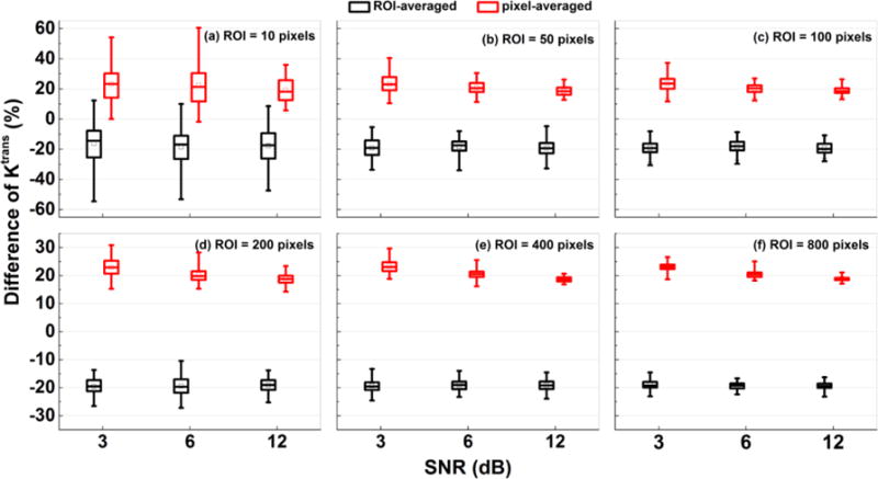
Box-plots of percentage differences of K^trans between the ‘true’ value, and the value obtained from ‘ROI-averaged’ analysis (black) and ‘pixel-averaged’ analysis (red) calculated for 100 simulations. The sizes of ROIs were (a) 10, (b) 50, (c) 100, (d) 200, (e) 400, and (f) 800 pixels. The squares indicate mean and bars indicate the upper and lower limits of the data. The percentage difference was calculated by: $\mathrm{\Delta }{K}^{\mathit{trans}}\left(\text{\%}\right)=\frac{K^{\mathit{trans}}\left(\text{Pixel}\text{or}\text{ROI}\right)-K^{\mathit{trans}}\left(\text{true}\right)}{K^{\mathit{trans}}\left(\text{true}\right)}\cdot 100\text{\%}.$

Similarly, Figure 4 shows the box-plots of percentage differences in v_e between the ‘true’ value, and the value obtained from ‘ROI-averaged’ analysis (black) and ‘pixel-averaged’ analysis (red) calculated for 100 simulations with added Gaussian noise of 3, 6, and 12 dB SNR for the ROIs containing: (a) 10, (b) 50, (c) 100, (d) 200, (e) 400, and (f) 800 different pixels. The v_e(Pixel) were closer to true v_e than the v_e(ROI) under the influences of noises. But on average, the v_e(ROI) were only about 7% underestimate true v_e.

Figure 4.

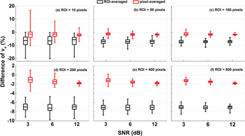
Box-plots of percentage differences of v_e between the ‘true’ value, and the value obtained from ‘ROI-averaged’ analysis (black) and ‘pixel-averaged’ analysis (red) calculated for 100 simulations. The sizes of ROIs were (a) 10, (b) 50, (c) 100, (d) 200, (e) 400, and (f) 800 pixels. The squares indicate mean and bars indicate the upper and lower limits of the data. The percentage difference was calculated by: $\mathrm{\Delta }{v}_e\left(\text{\%}\right)=\frac{v_e\left(\text{Pixel}\text{or}\text{ROI}\right)-v_e\left(\text{true}\right)}{v_e\left(\text{true}\right)}\cdot 100\text{\%}$

3.2. Animal experiments

For the center slice of the DCE-MRI dataset, Figure 5 shows the corresponding T2W images (left panel), K^trans(min⁻¹) maps (middle panel), and v_e maps (right panel) for six Copenhagen rats (a – f) that were implanted with AT2.1 prostate tumors in the hind limb. By visual inspection, the tumors K^trans and v_e were much more heterogeneous than muscle. The sizes of whole tumor ROIs (Fig. 5) ranged from 218 to 1257 pixels. The corresponding pixel histogram distributions of K^trans and v_e for six whole tumor ROIs (a – f) are shown in Figs. 6 and 7, respectively. There were variable distributions for both K^trans and v_e, for example, from Gaussian to right-skewed distributions, etc. But all of these distributions were different from the uniform distributions used in the simulations. Please notice that there were some pixels that had v_e close to 1, which indicated that the Tofts model is not optimal for these curves.

Figure 5.

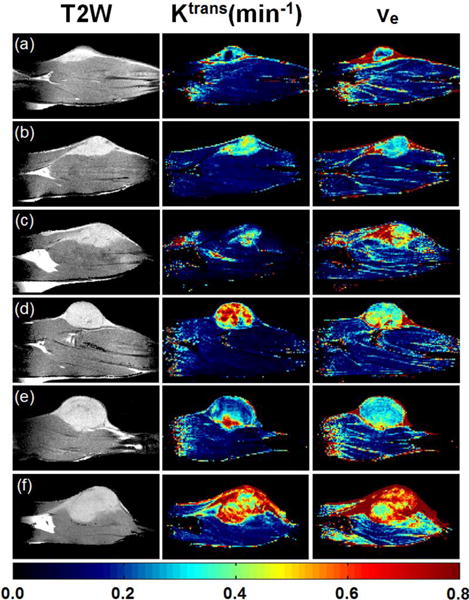
MRI and physiological parameter maps for six Copenhagen rats (a – f) that were implanted with AT2.1 prostate tumors on the hind limb for the center slices of DCE-MRI: T2W images (left panel), K^trans(min⁻¹) maps (middle panel) and v_e maps (right panel). The color bar indicates the values of maps. The displayed image FOV is 40.0 × 20.3 mm.

Figure 6.

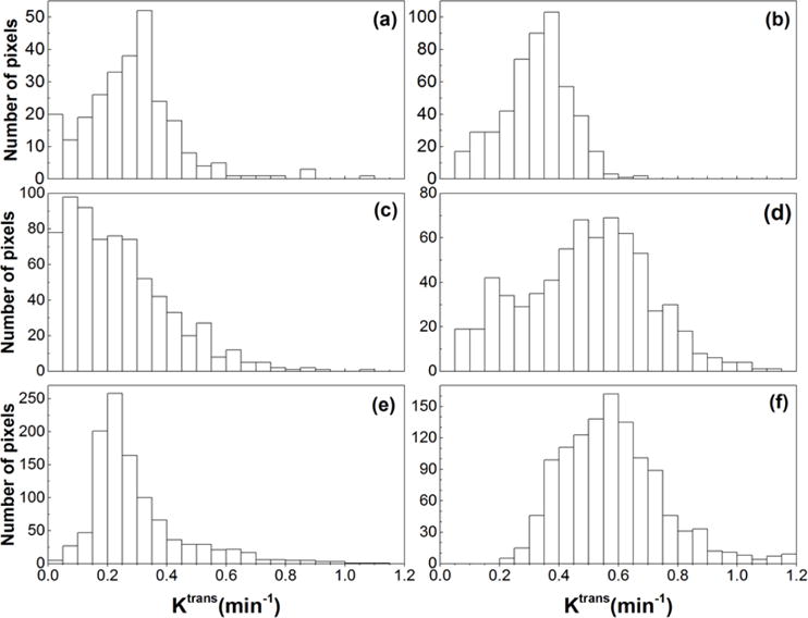
The histograms of tumor K^trans obtained from six Copenhagen rats with implanted prostate tumors shown in the Fig. 5 (a – f).

Figure 7.

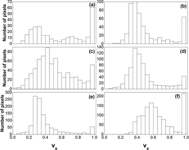
The histograms of tumor v_e obtained from six Copenhagen rats with implanted prostate tumors shown in the Fig. 5 (a – f).

Figure 8 shows the scatter plot of (a) K^trans(Pixel) vs. K^trans(ROI), and (b) v_e(Pixel) vs. v_e(ROI) obtained from tumor ROIs that were traced from three slices for each animal: (i) black squares for whole tumor, (ii) red open circles for rim, and (iii) green solid circles for core. On average, the K^trans(Pixel) was about 15% larger than the K^trans(ROI), and the v_e(Pixel) was about 10% larger than the v_e(ROI). However, there were some cases that v_e(Pixel) was smaller (on average ~15%) than the v_e(ROI), due to the fact that C(t) could not be accurately fitted by the Tofts model, for example, case (f) in the Fig. 5.

Figure 8.

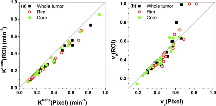
Scatter plots of (a) K^trans(Pixel) vs. K^trans(ROI) and (b) v_e(Pixel) vs. v_e(ROI) for six Copenhagen rats with implanted AT2.1 prostate tumors on the hind limb. The gray line is the line of equality. There are a total of 54 ROIs (6 animals × 3 slices × 3 ROIs (whole + rim + core)) containing 69 to 1257 pixels.

Finally, for three cases shown in the Fig. 8 with v_e(ROI) close to 1, Fig. 9 shows plots of measured C(t)_ROI (black dots) and corresponding fits (black line) obtained from the Tofts model. The plots demonstrate that the Tofts model could not fit these C(t)_ROI accurately, unless values of v_e larger than 1 were allowed. The extracted K^trans(ROI) for these three cases (a – c) was 0.50, 0.52, and 0.69 min⁻¹, respectively.

Figure 9.

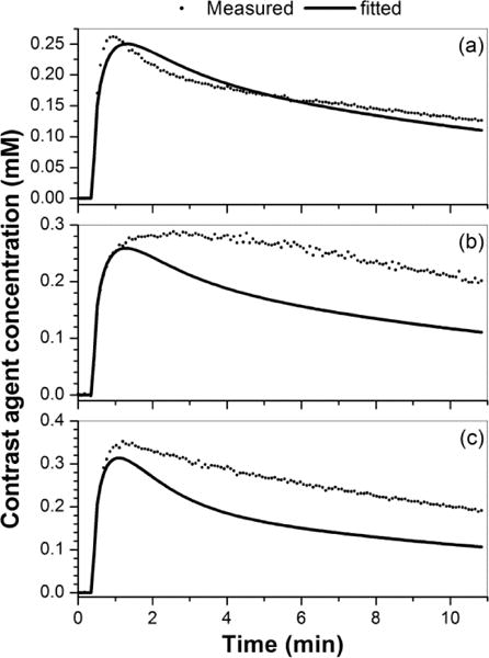
Plots of contrast agent concentration versus time curves (a – c) measured from tumor ROIs (dots) and corresponding fitted curves (line) obtained with the Tofts model for three cases shown in Fig. 8 with v_e(ROI) close to 1 (from left to right).

4. Discussion

Our simulations showed that the K^trans(ROI) was significantly underestimated the K^trans(Pixel). When the size of the ROI increased, the spread of K^trans and v_e values was reduced for 100 simulations, but the degree of underestimation is still significant between pixel and ROI based analysis. This is understandable because the averaging of parameters over a large ROI reduces the variations, and averaging the C(t) over a large ROI would be much smoother than the individual curve. The pixel based analysis would be much more influenced by individual pixels, especially for small size of ROI. These findings were true for both simulated noise free and added noise contrast agent concentration curves. Despite significant differences between ‘pixel-averaged’ and ‘ROI-averaged’ analysis, the simulation results showed that there were strong positive linear correlations between the two types of analysis for both K^trans and v_e values. This information could be valuable when comparing ‘pixel-averaged’ and ‘ROI-averaged’ analysis from different sites.

The simulation results also showed that added noise had a greater effect on K^trans (Fig. 1) but less effect on v_e (Fig. 2). This could be explained by the roles of K^trans and v_e in the Tofts model. The Tofts model can be considered as the AIF (C_p(t)) convoluted with an exponential decay function, i.e., $C\left(t\right)=C_p\left(t\right)\otimes K^{\mathit{trans}}\cdot \text{exp}\left(-t\cdot K^{\mathit{trans}}/v_e\right)$. Therefore, K^trans is influenced more by earlier uptake of contrast agent, while v_e is influenced more by the later washout of contrast agent. The extracted physiological parameters ( ${\stackrel{\sim }{K}}^{\mathit{trans}}$ and ${\stackrel{\sim }{v}}_e$) for noisy curves $\stackrel{\sim }{C}\left(t\right)=C\left(t\right)+n\left(t\right)$ can be approximately related to physiological parameters (K^trans and v_e) for noise free curves C(t), as follows (please see detailed derivations in Appendix A):

$${\stackrel{\sim }{K}}^{\text{trans}}\approx K^{\text{trans}}+\left(dn\left(t\right)/dt\right)/C_{\mathrm{p}}\left(t\right),\text{for}\mathrm{t}\ll 1\text{and}{\stackrel{\sim }{v}}_e\approx v_e+n\left(t\right)/C_p\left(t\right),\text{for}\mathrm{t}\gg 1.$$

Therefore, ${\stackrel{\sim }{K}}^{\text{trans}}$ is influenced by the derivative of noise, but noise simply adds to ${\stackrel{\sim }{v}}_e$. The addition of the derivative of noise to K^trans amplifies the effect of noise. This is the reason why added noise had more influence on K^trans than v_e in our simulation studies. Under the influence of noise, and considering the average parameters generated by the simulation as the ‘true’ physiological parameters for the ROI, our results show that K^trans(Pixel) was greater than the ‘true’ K^trans, but the K^trans(ROI) was less than the ‘true’ K^trans. The K^trans(ROI) was closer to the true K^trans than K^trans(Pixel) for high noise levels. Therefore, the noise has a greater effect on K^trans for pixel-averaged analysis than ROI-averaged analysis.

The K^trans and v_e maps derived from the implanted prostate tumors DCE-MRI data were more heterogeneous than the leg muscles. The values of K^trans obtained from ‘pixel-averaged’ and ‘ROI-averaged’ analysis of real data from the tumors were much closer than our simulation results predicted. On the other hand, the values of v_e obtained from ‘pixel-averaged’ and ‘ROI-averaged’ analysis of real data from the tumors were more different than our simulation results predicted. This could be due to the non-uniform pixel distributions of K^trans and v_e within the tumor, in contrast to the uniform distributions of K^trans and v_e used in the simulation study. Importantly, in some pixels’ and/or ROIs’, the contrast agent concentration curves for tumors could not be accurately fitted by the Tofts model. This was evidenced by the v_e values that were close to 1 on the maps or on histograms, and as shown in Fig. 8. Therefore, perfusion and capillary permeability may be very heterogeneous even within individual small pixels for the cancers. In principal, heterogeneity can produce a ‘plateau’ or ‘persistent’ kinetic curve, due to a large range of K^trans and v_e values within a ROI. Please note that the necrotic tissue could also produce a curve with larger v_e, but in this case, a smaller K^trans would be expected (Barnes et al., 2012), and this was not the case in the examples shown in Fig. 9.

Our animal experiments found differences between pixel- and ROI-based analysis that were slightly greater than those found in a previous study (Ng et al., 2015). Our implanted prostate tumors had larger ranges of physiological parameters (K^trans and v_e) than those that Ng et al. (Ng et al., 2015) observed. This could be due to differences in the tumor type, location of the tumor, and the AIF. The pixel-by-pixel analysis (compared to ROI) was better able to capture the heterogeneity of the tumor (Haney et al., 2013). Therefore, when there is sufficient SNR, the best approach would clearly be a pixel-based analysis with the subsequent histogram analysis. For heterogeneous tumors, the median of the perfusion parameter would be a more appropriate diagnostic parameter rather than the average perfusion parameter estimated from pixel-based analysis because of the generally nonsymmetrical distributions of K^trans and v_e over the ROI.

Our conclusions are based on a limited number of computer simulations and implanted AT2.1 prostate tumor experiment results. This study could not cover all possible scenarios; this is the main limitation of this study. The simulation study did not include C(t) plots with an initial rapid uptake of contrast agent followed by a prolonged slow uptake of the contrast agent, even though these curves are commonly observed in practice, because the Tofts model could not generate this type of curve. For animal experiments, only one type of tumor cell-line was used. However, for human prostate cancer in mouse xenograft models, it is known that different cell lines may lead to different microvascular density (MVD) (Rofstad and Mathiesen, 2010). Some cell lines may show higher vascular density in the center and lower in periphery, such as DU-145 cell line; and others show homogeneous MVD, such as human prostate cancer PC-3 cell lines (Saidov et al., 2016, Farace et al., 2011, Pang et al., 2011). Extracted physiological parameters could be impacted by spatial distribution of MVD within the tumor ROI.

In conclusion, the results reported here demonstrate that heterogeneity leads to poor fits to DCE-MRI data, and errors in extracting K^trans and v_e. Similar errors may arise from heterogeneity of perfusion and capillary permeability within individual pixels. This limits the diagnostic accuracy of the parameters derived from the Tofts model. To increase the sensitivity and specificity of cancer diagnosis using DCE-MRI, ‘pixel-averaged’ analysis may be preferable for extraction of accurate physiological parameters from heterogeneous tumors. The ‘ROI-averaged’ analysis should only be used when there is low SNR for DCE-MRI data.

Appendix A

In our simulation studies, the noise curve $\stackrel{\sim }{C}\left(t\right)$ was obtained by adding noise n(t) to a noise free curve C(t). Then the Tofts model was used to fit the $\stackrel{\sim }{C}\left(t\right)$ to extract ${\stackrel{\sim }{K}}^{\text{trans}}$ and ${\stackrel{\sim }{v}}_e$ for the noisy curve, i.e.,

$$\stackrel{\sim }{C}\left(t\right)={\stackrel{\sim }{K}}^{\text{trans}}{\displaystyle {\int }_0^t{C}_{\mathrm{p}}\left(\tau \right)\text{exp}\left(-\left(t-\tau \right){\stackrel{\sim }{K}}^{\text{trans}}/{\stackrel{\sim }{v}}_e\right)d\tau =K^{\text{trans}}{\displaystyle {\int }_0^t{C}_{\mathrm{p}}\left(\tau \right)\text{exp}\left(-\left(t-\tau \right)K^{\text{trans}}/v_e\right)d\tau +n\left(t\right).}}$$ (A1)

At earlier times after injection (t ≪1), the efflux of the contrast agent from the extravascular extracellular space (EES) back to plasma is negligible, and above Eq. (A1) can be simplified as follows:

$$\stackrel{\sim }{C}\left(t\right)\approx {\stackrel{\sim }{K}}^{\text{trans}}{\displaystyle {\int }_0^t{C}_{\mathrm{p}}\left(\tau \right)}d\tau \approx K^{\text{trans}}{\displaystyle {\int }_0^t{C}_{\mathrm{p}}\left(\tau \right)}d\tau +n\left(t\right),\text{for t<<1}.$$ (A2)

By taking the derivatives respect to time on both sides of Eq. (A2), the following Eq. (A3) can be obtained:

$${\stackrel{\sim }{K}}^{\text{trans}}{C}_{\mathrm{p}}\left(t\right)\approx K^{\text{trans}}{C}_{\mathrm{p}}\left(t\right)+dn\left(t\right)/dt,\text{for t<<1}.$$ (A3)

From Eq. (A3), ${\stackrel{\sim }{K}}^{\text{trans}}$ can be solved:

$${\stackrel{\sim }{K}}^{\text{trans}}\approx K^{\text{trans}}+\left(dn\left(t\right)/dt\right)/C_{\mathrm{p}}\left(t\right),\text{for t<<1}.$$ (A4)

Therefore, ${\stackrel{\sim }{K}}^{\text{trans}}$ is influenced by the derivative of noise, which would amplify the effects of noise.

In order to explain the noise effects on v_e, the derivative form of the Tofts model was considered:

$$dC\left(t\right)/dt=K^{\mathit{trans}}\left(C_p\left(t\right)-C\left(t\right)/v_e\right).$$ (A5)

At later time after injection (t >>1), it’s a good approximation that dC(t)/dt ≈ 0, because C(t) changes much more slower than at earlier times (Fan et al., 2010). Then Eq. (A5) can be simplified as follows:

$$0\approx K^{\mathit{trans}}\left(C_p\left(t\right)-C\left(t\right)/v_e\right),\Rightarrow C\left(t\right)\approx v_e{C}_p\left(t\right),\text{for t>>1}.$$ (A6)

By using Eq. (A6), with added noise $\stackrel{\sim }{C}\left(t\right)$ and ${\stackrel{\sim }{v}}_e$ can be related to noise free C(t) and v_e, i.e.,

$$\stackrel{\sim }{C}\left(t\right)\approx {\stackrel{\sim }{v}}_e{C}_p\left(t\right)\approx C\left(t\right)+n\left(t\right)\approx v_e{C}_p\left(t\right)+n\left(t\right),\text{for t>>1}.$$ (A7)

From Eq. (A7), ${\stackrel{\sim }{v}}_e$ can be determined:

$${\stackrel{\sim }{v}}_e\approx v_e+n\left(t\right)/C_p\left(t\right),\text{for t>>1}.$$ (A8)

Therefore, noise simply adds to ${\stackrel{\sim }{v}}_e$ and this effect is much smaller than the effect of the derivative of noise added to ${\stackrel{\sim }{K}}^{\text{trans}}$.

References

- Ahearn TS, Staff RT, Redpath TW, Semple SI. The use of the Levenberg-Marquardt curve-fitting algorithm in pharmacokinetic modelling of DCE-MRI data. Phys Med Biol. 2005;50:N85–92. doi: 10.1088/0031-9155/50/9/N02. [DOI] [PubMed] [Google Scholar]
- Alonzi R, Taylor NJ, Stirling JJ, D’arcy JA, Collins DJ, Saunders MI, Hoskin PJ, Padhani AR. Reproducibility and correlation between quantitative and semiquantitative dynamic and intrinsic susceptibility-weighted MRI parameters in the benign and malignant human prostate. J Magn Reson Imaging. 2010;32:155–64. doi: 10.1002/jmri.22215. [DOI] [PubMed] [Google Scholar]
- Barnes SL, Whisenant JG, Loveless ME, Yankeelov TE. Practical dynamic contrast enhanced MRI in small animal models of cancer: data acquisition, data analysis, and interpretation. Pharmaceutics. 2012;4:442–78. doi: 10.3390/pharmaceutics4030442. [DOI] [PMC free article] [PubMed] [Google Scholar]
- Chen YJ, Chu WC, Pu YS, Chueh SC, Shun CT, Tseng WY. Washout gradient in dynamic contrast-enhanced MRI is associated with tumor aggressiveness of prostate cancer. J Magn Reson Imaging. 2012;36:912–9. doi: 10.1002/jmri.23723. [DOI] [PubMed] [Google Scholar]
- Dale BM, Jesberger JA, Lewin JS, Hillenbrand CM, Duerk JL. Determining and optimizing the precision of quantitative measurements of perfusion from dynamic contrast enhanced MRI. J Magn Reson Imaging. 2003;18:575–84. doi: 10.1002/jmri.10399. [DOI] [PubMed] [Google Scholar]
- Engelbrecht MR, Huisman HJ, Laheij RJ, Jager GJ, Van Leenders GJ, Hulsbergen-Van De Kaa CA, De La Rosette JJ, Blickman JG, Barentsz JO. Discrimination of prostate cancer from normal peripheral zone and central gland tissue by using dynamic contrast-enhanced MR imaging. Radiology. 2003;229:248–54. doi: 10.1148/radiol.2291020200. [DOI] [PubMed] [Google Scholar]
- Fan X, Haney CR, Mustafi D, Yang C, Zamora M, Markiewicz EJ, Karczmar GS. Use of a reference tissue and blood vessel to measure the arterial input function in DCEMRI. Magn Reson Med. 2010;64:1821–6. doi: 10.1002/mrm.22551. [DOI] [PMC free article] [PubMed] [Google Scholar]
- Farace P, Merigo F, Fiorini S, Nicolato E, Tambalo S, Daducci A, Degrassi A, Sbarbati A, Rubello D, Marzola P. DCE-MRI using small-molecular and albumin-binding contrast agents in experimental carcinomas with different stromal content. Eur J Radiol. 2011;78:52–9. doi: 10.1016/j.ejrad.2009.04.043. [DOI] [PubMed] [Google Scholar]
- Franiel T, Hamm B, Hricak H. Dynamic contrast-enhanced magnetic resonance imaging and pharmacokinetic models in prostate cancer. Eur Radiol. 2011;21:616–26. doi: 10.1007/s00330-010-2037-7. [DOI] [PubMed] [Google Scholar]
- Guo JY, Reddick WE. DCE-MRI pixel-by-pixel quantitative curve pattern analysis and its application to osteosarcoma. J Magn Reson Imaging. 2009;30:177–84. doi: 10.1002/jmri.21785. [DOI] [PubMed] [Google Scholar]
- Haney CR, Fan X, Markiewicz E, Mustafi D, Karczmar GS, Stadler WM. Monitoring anti-angiogenic therapy in colorectal cancer murine model using dynamic contrast-enhanced MRI: comparing pixel-by-pixel with region of interest analysis. Technol Cancer Res Treat. 2013;12:71–8. doi: 10.7785/tcrt.2012.500255. [DOI] [PubMed] [Google Scholar]
- Hectors SJ, Besa C, Wagner M, Jajamovich GH, Haines GK, 3rd, Lewis S, Tewari A, Rastinehad A, Huang W, Taouli B. DCE-MRI of the prostate using shutter-speed vs. Tofts model for tumor characterization and assessment of aggressiveness. J Magn Reson Imaging. 2017 doi: 10.1002/jmri.25631. [DOI] [PubMed] [Google Scholar]
- Heisen M, Fan X, Buurman J, Van Riel NA, Karczmar GS, Ter Haar Romeny BM. The use of a reference tissue arterial input function with low-temporal-resolution DCE-MRI data. Phys Med Biol. 2010;55:4871–83. doi: 10.1088/0031-9155/55/16/016. [DOI] [PubMed] [Google Scholar]
- Hotker AM, Mazaheri Y, Zheng J, Moskowitz CS, Berkowitz J, Lantos JE, Pei X, Zelefsky MJ, Hricak H, Akin O. Prostate Cancer: assessing the effects of androgen-deprivation therapy using quantitative diffusion-weighted and dynamic contrast-enhanced MRI. Eur Radiol. 2015;25:2665–72. doi: 10.1007/s00330-015-3688-1. [DOI] [PMC free article] [PubMed] [Google Scholar]
- Langer DL, Van Der Kwast TH, Evans AJ, Trachtenberg J, Wilson BC, Haider MA. Prostate cancer detection with multi-parametric MRI: logistic regression analysis of quantitative T2, diffusion-weighted imaging, and dynamic contrast-enhanced MRI. J Magn Reson Imaging. 2009;30:327–34. doi: 10.1002/jmri.21824. [DOI] [PubMed] [Google Scholar]
- Lavini C, Pikaart BP, De Jonge MC, Schaap GR, Maas M. Region of interest and pixel-by-pixel analysis of dynamic contrast enhanced magnetic resonance imaging parameters and time-intensity curve shapes: a comparison in chondroid tumors. Magn Reson Imaging. 2009;27:62–8. doi: 10.1016/j.mri.2008.05.012. [DOI] [PubMed] [Google Scholar]
- Leach MO, Morgan B, Tofts PS, Buckley DL, Huang W, Horsfield MA, Chenevert TL, Collins DJ, Jackson A, Lomas D, Whitcher B, Clarke L, Plummer R, Judson I, Jones R, Alonzi R, Brunner T, Koh DM, Murphy P, Waterton JC, Parker G, Graves MJ, Scheenen TW, Redpath TW, Orton M, Karczmar G, Huisman H, Barentsz J, Padhani A. Imaging vascular function for early stage clinical trials using dynamic contrast-enhanced magnetic resonance imaging. Eur Radiol. 2012;22:1451–64. doi: 10.1007/s00330-012-2446-x. [DOI] [PubMed] [Google Scholar]
- Li X, Cai Y, Moloney B, Chen Y, Huang W, Woods M, Coakley FV, Rooney WD, Garzotto MG, Springer CS., Jr Relative sensitivities of DCE-MRI pharmacokinetic parameters to arterial input function (AIF) scaling. J Magn Reson. 2016;269:104–12. doi: 10.1016/j.jmr.2016.05.018. [DOI] [PMC free article] [PubMed] [Google Scholar]
- Mehrabian H, Da Rosa M, Haider MA, Martel AL. Pharmacokinetic analysis of prostate cancer using independent component analysis. Magn Reson Imaging. 2015;33:1236–45. doi: 10.1016/j.mri.2015.08.009. [DOI] [PubMed] [Google Scholar]
- Ng CS, Wei W, Bankson JA, Ravoori MK, Han L, Brammer DW, Klumpp S, Waterton JC, Jackson EF. Dependence of DCE-MRI biomarker values on analysis algorithm. PLoS One. 2015;10:e0130168. doi: 10.1371/journal.pone.0130168. [DOI] [PMC free article] [PubMed] [Google Scholar]
- O’connor JP, Jackson A, Parker GJ, Roberts C, Jayson GC. Dynamic contrast-enhanced MRI in clinical trials of antivascular therapies. Nat Rev Clin Oncol. 2012;9:167–77. doi: 10.1038/nrclinonc.2012.2. [DOI] [PubMed] [Google Scholar]
- Ocak I, Bernardo M, Metzger G, Barrett T, Pinto P, Albert PS, Choyke PL. Dynamic contrast-enhanced MRI of prostate cancer at 3 T: a study of pharmacokinetic parameters. AJR Am J Roentgenol. 2007;189:849. doi: 10.2214/AJR.06.1329. [DOI] [PubMed] [Google Scholar]
- Othman AE, Falkner F, Martirosian P, Schraml C, Schwentner C, Nickel D, Nikolaou K, Notohamiprodjo M. Optimized Fast Dynamic Contrast-Enhanced Magnetic Resonance Imaging of the Prostate: Effect of Sampling Duration on Pharmacokinetic Parameters. Invest Radiol. 2016;51:106–12. doi: 10.1097/RLI.0000000000000213. [DOI] [PubMed] [Google Scholar]
- Pang X, Wu Y, Lu B, Chen J, Wang J, Yi Z, Qu W, Liu M. (-)-Gossypol suppresses the growth of human prostate cancer xenografts via modulating VEGF signaling-mediated angiogenesis. Mol Cancer Ther. 2011;10:795–805. doi: 10.1158/1535-7163.MCT-10-0936. [DOI] [PMC free article] [PubMed] [Google Scholar]
- Parker GJ, Roberts C, Macdonald A, Buonaccorsi GA, Cheung S, Buckley DL, Jackson A, Watson Y, Davies K, Jayson GC. Experimentally-derived functional form for a population-averaged high-temporal-resolution arterial input function for dynamic contrast-enhanced MRI. Magn Reson Med. 2006;56:993–1000. doi: 10.1002/mrm.21066. [DOI] [PubMed] [Google Scholar]
- Rofstad EK, Mathiesen B. Metastasis in melanoma xenografts is associated with tumor microvascular density rather than extent of hypoxia. Neoplasia. 2010;12:889–98. doi: 10.1593/neo.10712. [DOI] [PMC free article] [PubMed] [Google Scholar]
- Saidov T, Heneweer C, Kuenen M, Von Broich-Oppert J, Wijkstra H, Rosette J, Mischi M. Fractal Dimension of Tumor Microvasculature by DCE-US: Preliminary Study in Mice. Ultrasound Med Biol. 2016;42:2852–2863. doi: 10.1016/j.ultrasmedbio.2016.08.001. [DOI] [PubMed] [Google Scholar]
- Tofts PS, Brix G, Buckley DL, Evelhoch JL, Henderson E, Knopp MV, Larsson HB, Lee TY, Mayr NA, Parker GJ, Port RE, Taylor J, Weisskoff RM. Estimating kinetic parameters from dynamic contrast-enhanced T(1)-weighted MRI of a diffusable tracer: standardized quantities and symbols. J Magn Reson Imaging. 1999;10:223–32. doi: 10.1002/(sici)1522-2586(199909)10:3<223::aid-jmri2>3.0.co;2-s. [DOI] [PubMed] [Google Scholar]
- Tokuda J, Mamata H, Gill RR, Hata N, Kikinis R, Padera RF, Jr, Lenkinski RE, Sugarbaker DJ, Hatabu H. Impact of nonrigid motion correction technique on pixel-wise pharmacokinetic analysis of free-breathing pulmonary dynamic contrast-enhanced MR imaging. J Magn Reson Imaging. 2011;33:968–73. doi: 10.1002/jmri.22490. [DOI] [PMC free article] [PubMed] [Google Scholar]