Random Partition Distribution Indexed by Pairwise Information

Abstract

We propose a random partition distribution indexed by pairwise similarity information such that partitions compatible with the similarities are given more probability. The use of pairwise similarities, in the form of distances, is common in some clustering algorithms (e.g., hierarchical clustering), but we show how to use this type of information to define a prior partition distribution for flexible Bayesian modeling. A defining feature of the distribution is that it allocates probability among partitions within a given number of subsets, but it does not shift probability among sets of partitions with different numbers of subsets. Our distribution places more probability on partitions that group similar items yet keeps the total probability of partitions with a given number of subsets constant. The distribution of the number of subsets (and its moments) is available in closed-form and is not a function of the similarities. Our formulation has an explicit probability mass function (with a tractable normalizing constant) so the full suite of MCMC methods may be used for posterior inference. We compare our distribution with several existing partition distributions, showing that our formulation has attractive properties. We provide three demonstrations to highlight the features and relative performance of our distribution.

1. Introduction

We propose a random partition distribution indexed by pairwise information for flexible Bayesian modeling. By way of introduction, consider Gibbs-type priors (De Blasi et al. 2015) which lead to a broad class of Bayesian nonparametric models for data y₁, y₂…:

$$y_i|{\theta }_i~p\left(y_i|{\theta }_i\right),{\theta }_i|F~F,F~Q,$$ (1)

where p(y| θ) is a sampling distribution indexed by θ, F is a discrete random probability measure, and Q is an infinite-dimensional prior distribution termed the de Finetti measure. The model can be enriched by indexing the sampling model by other parameters or by placing priors on hyperparameters defining the prior distribution Q. The sequence θ ₁, θ₂,… in (1) is exchangeable and the discrete nature of F implies that θ₁, θ₂,… will have ties with positive probability. Therefore, for any finite n, we can reparameterize θ ₁, …, θ_n in terms of the unique values $\varphi =\left({\varphi }_1,\dots ,{\varphi }_{q_n}\right)$ and a partition ${\pi }_n=\left\{S_1,\dots ,S_{q_n}\right\}$, a set whose subsets $S_1,\dots ,S_{q_n}$ are nonempty, mutually exclusive, and exhaustive such that ${\cup }_{S\in {\pi }_n}S=\left\{1,\dots ,n\right\}$. Two integers i and i′ belong to S_j if and only if θ_i = θ_i′ = ϕ_j. The parameters ${\varphi }_1,\dots ,{\varphi }_{q_n}$ are independent and identically distributed G0, the centering distribution of Q. F in (1) implies a prior on π_n having support ${ℱ}_n$ (the set of all possible partitions of n items). A distribution over ${ℱ}_n$ is discrete, but the size of the space — which grows according to the Bell (1934) number — makes exhaustive calculations impossible except for very small n.

The choice of Q leads to different exchangeable random partition models. For example, when Q is the Dirichlet process (Ferguson 1973), the partition distribution p(π_n) is the Ewens distribution (Ewens 1972; Pitman 1995, 1996) and the model in (1) is a Dirichlet process mixture model (Antoniak 1974). Or, when Q is the Poisson-Dirichlet process (Pitman and Yor 1997), the partition distribution p(π_n) is the Ewens-Pitman distribution (Pitman and Yor 1997) and the model in (1) is a Poisson-Dirichlet process mixture model.

In some situations, the random probability measure F and the de Finetti measure Q are not of interest and the model in (1) maybe marginalized as:

$$y_i|{\theta }_i~p\left(y_i|{\theta }_i\right),{\theta }_i={\displaystyle \sum _{j=1}^{q_n}{\varphi }_{j}I\left\{i\in S_j\right\},}{\varphi }_j~G_0,{\pi }_n~p\left({\pi }_n\right).$$ (2)

Popular models for the partition distribution p(π_n) include product partition models, species sampling models, and model-based clustering. These are reviewed by Quintana (2006) and Lau and Green (2007).

Exchangeable random partition models, which follow from the formulation in (1), have many attractive properties. For example, in exchangeable random partition models, the sequence of partition distributions with increasing sample size is marginally invariant: The partition distribution of n items is identical to the marginal distribution of the first n items after integrating out the last observation in the partition distribution of n + 1 items. Insisting on an exchangeable random partition distribution, however, imposes limits of the formulation of partition distributions (Lee et al. 2013).

The presence of item-specific information makes the exchangeability assumption on θ₁,…, θ_n unreasonable. Indeed the aim of this article is to explicitly explore a random probability model for partitions that uses pairwise information to a priori influence the partitioning. Since our partition distribution is nonexchangeable, there is no notion of an underlying de Finetti measure Q giving rise to our partition distribution and our model lacks marginal invariance. We will show, however, how to make the data analysis invariant to the order in which the data are observed. The use of pairwise distances is common in many ad hoc clustering algorithms (e.g., hierarchical clustering), but we show how to use this type of information to define a prior partition distribution for flexible Bayesian modeling.

Recent work has developed other nonexchangeable random partition models. A common thread is the use of covariates to influence a priori the probability for random partitions. Park and Dunson (2010) and Shahbaba and Neal (2009) include clustering covariates as part of an augmented response vector to obtain a prior partition model for inference on the response data. Park and Dunson (2010) build on product partition models and focus on continuous covariates treated as random variables, whereas Shahbaba and Neal (2009) use the Dirichlet process as the random partition and model a categorical response with logistic regression. Müller, Quintana, and Rosner (2011) proposed the PPMx model, a product partition model with covariates. In their simulation study of several of these approaches, they found no dominant method and suggested choosing among them based on the inferential goals. More recently, Airoldi et al. (2014) provided a general family of nonexchangeable species sampling sequences dependent on the realizations of a set of latent variables.

Our proposed partition distribution—which we call the Ewens-Pitman attraction (EPA) distribution—is indexed by pairwise similarities among the items, as well as a mass parameter α and a discount parameter δ which control the distribution of the number of subsets and the distribution of subset sizes. Our distribution allocates items based on their attraction to existing subsets, where the attraction to a given subset is a function of the pairwise similarities between the current item and the items in the subset. A defining feature of our distribution is that it allocates probability among partitions within a given number of subsets, but it does not shift probability among sets of partitions with different numbers of subsets. The distribution of the number of subsets (and its moments) induced by our distribution is available in closed-form and is invariant to the similarity information.

We compare our EPA distribution with several existing distributions. We draw connections with the Ewens and Ewens-Pitman distributions which result from the Dirichlet process (Ferguson 1973) and Pitman-Yor process (Pitman and Yor 1997), respectively. Of particular interest are the distributions in the proceedings article of Dahl (2008) and the distance dependent Chinese restaurant process (ddCRP) of Blei and Frazier (2011). Whereas our distribution directly defines a distribution over partitions through sequential allocation of items to subsets in a partition, both Dahl (2008) and Blei and Frazier (2011) implicitly define the probability of a partition by summing up the probabilities of all associated directed graphs whose nodes each have exactly one edge or loop. We will see that, although these other distributions use the same similarity information, our distributions behavior is substantially different. We will also contrast our approach with the PPMx model of Müller, Quintana, and Rosner (2011). Unlike the ddCRP and PPMx distributions, our partition distribution has both an explicit formula for the distribution of the number of subsets and a probability mass function with a tractable normalizing constant. As such, standard MCMC algorithms may be easily applied for posterior inference on the partition π_n and any hyperparameters that influence partitioning. A demonstration, an application, and a simulation study all help to show the properties of our proposal and investigate its performance relative to leading alternatives.

2. Ewens-Pitman Attraction Distribution

2.1. Allocating Items According to a Permutation

Our EPA distribution can be described as sequentially allocating items to subsets to form a partition. The order in which items are allocated is not necessarily their order in the dataset; the permutation σ = (σ₁, …, σ_n) of {1, …, n} gives the sequence in which the n items are allocated, where the t th item allocated is σ_t. The sequential allocation of items yields a sequence of partitions and we let π(σ₁, …, σ_t−1) denote the partition of {σ₁, …, σ_t−1} at time t − 1. Let q_t−1 denote the number of subsets in π(σ₁,…, σ_t−1). For t = 1, we take {σ₁,…, σ₁₋₁} to mean the empty set and item σ₁ is allocated to a new subset. At time t > 1, item σ_t is allocated to one of the q_t−1 subsets in π(σ₁, …, σ_t−1) or is allocated to a new subset. If S denotes the subset to which item σ_t will be allocated, then the partition at time t is obtained from the partition at time t − 1 as follows: π(σ₁, …, σ_t) = (π(σ₁, …, σ_t−1) \ {S}) ∪ S ∪ {σ_t}}. Note that π (σ₁, …, σ_n) is equivalent to the partition π_n.

The permutation σ can be fixed (e.g., in the order the observations are recorded). Note, however, that our partition distribution does indeed depend on the permutation σ and it can be awkward that a data analysis depends on the order the data are processed. We recommend using the uniform distribution on the permutation, that is, p(σ) = 1/n! for all σ. This has the effect of making analyses using the EPA distribution symmetric with respect to permutation of the sample indices, that is, the data analysis then does not depend on the order of the data.

2.2. Pairwise Similarity Function and Other Parameters

Our proposed EPA distribution uses available pairwise information to influence the partitioning of items. In its most general form, this pairwise information is represented by a similarity function λ. such that λ(i, j) > 0 for any i, j ∈ {1, …, n} and λ(i, j) = λ(j, i). We note that the similarity function can involve unknown parameters and we later discuss how to make inference on these parameters. A large class of similarity functions can be defined as λ (i, j) = f(d_ij), where f is a nonincreasing function of pairwise distances d_ij between items i and j. The metric defining the pairwise distances and the functional form of f are modeling choices. For example, the reciprocal similarity is f(d) = d^−τ for d > 0. If d_ij = 0 for some i ≠ j, one could add a small constant to the distances or consider another similarity function such as the exponential similarity f(d) = exp(−τd). We call the exponent τ ≥ 0 the temperature, as it has the effect of dampening or accentuating the distances. In addition to σ and λ, the EPA distribution is also indexed by a discount parameter δ ∈ [0, 1) and a mass parameter α > −δ, which govern distribution of the number of subsets and distribution of subset sizes.

2.3. Probability Mass Function

The probability mass function (p.m.f.) for a partition π_n having the EPA distribution is the product of increasing conditional probabilities:

$$p\left({\pi }_n|\alpha ,\delta ,\lambda ,\sigma \right)={\displaystyle \prod _{t=1}^n{p}_t\left(\alpha ,\delta ,\lambda ,\pi \left({\sigma }_1,\dots ,{\sigma }_{t-1}\right)\right),}$$ (3)

where p_t(α, δ, λ, π(σ ₁, …, σ_t−1)) is one for t = 1 and is otherwise defined as

$$p_t\left(\alpha ,\delta ,\lambda ,\pi \left({\sigma }_1,\dots ,{\sigma }_{t-1}\right)\right)=\text{pr}\left({\sigma }_t\in S|\alpha ,\delta ,\lambda ,\pi \left({\sigma }_1,\dots ,{\sigma }_{t-1}\right)\right)=\{\begin{array}{l}\frac{t-1-\delta q_{t-1}}{\alpha +t-1}\cdot \frac{{\sum }_{{\sigma }_s\in S}\lambda \left({\sigma }_t,{\sigma }_s\right)}{{\displaystyle {\sum }_{s=1}^{t-1}\lambda \left({\sigma }_t,{\sigma }_s\right)}}\text{for }S\in \pi \left({\sigma }_1,\dots ,{\sigma }_{t-1}\right)\\ \frac{\alpha +{\delta }_{qt-1}}{\alpha +t-1}\text{for }S\text{ being a new subset}.\end{array}$$ (4)

At each step, ${\displaystyle {\sum }_{s=1}^{t-1}\lambda \left({\sigma }_t,{\sigma }_s\right)}$ is the total attraction of item σ_t to the previously allocated items. The ratio of the sums of the similarity function λ in (4) gives the proportion of the total attraction of item σ_t to those items allocated to subset S. As such, item σ_t is likely to be allocated to a subset having items to which it is attracted. We note that our distribution is invariant to scale changes in the similarity λ, which aligns with the idea that similarity is a relative rather than an absolute concept.

2.4. Marginal Invariance

A sequence of random partition distributions in the sample size n is marginally invariant (also known as consistent or coherent) if the probability distribution for partitions of {1, …, n} is the same as the distribution obtained by marginalizing out n + 1 from the probability distribution for partitions of {1, …, n + 1}. For a nontrivial similarity function λ, the proposed EPA distribution is not marginally invariant. We argue, however, that insisting on marginal invariance is too limiting in the context of pairwise similarity information.

Consider the following simple example with n = 3 items. Let p₀ be the partition distribution for π₃ obtained from (3), let p₁ be the distribution of the partition π₂ obtained by marginalizing p₀ over item 3, and let p₂ be the distribution of the partition π₂ in (3) assuming n = 2. Without loss of generality, assume α = 1, λ(1, 2) = 1, λ(1, 3) = a, and λ(2, 3) = b. Using reciprocal similarity (i.e., distances 1/a and 1/b) and the uniform distribution on the permutation σ, algebra shows that marginal invariance requires the similarities a and b are reciprocals of each other. This constraint is displayed graphically in Figure 1. Whereas one would like to be able to consider any placement of x₃, marginal invariance requires that x₃ lie on the Cassini oval. The conclusion is that requiring marginal invariance severely constrains the similarity information in ways that are not likely to be seen in practice. Of course, saying that two items are similar is relative to the other items being considered and, hence, the distribution should be allowed to change as more items are added. Marginal invariance should not be expected, or imposed, in the presence of pairwise similarity information. As such, a data analysis based on n observations using our EPA distribution should be viewed as an analysis of just those observations.

Figure 1.

While ideally item 3 could be placed anywhere, insisting on marginal invariance for the EPA distribution requires that item 3 be constrained to fall on this Cassini oval.

2.5. Distributions on the Parameters

The EPA distribution is indexed by the mass parameter α, the discount parameter δ, the similarity function λ, and the permutation σ. These parameters can be treated as known fixed quantities, or they may be treated as unknown random quantities having distributions. The values at which they are fixed or their distributions are modeling choices. Here we give some suggestions. We recommend a gamma distribution for the mass parameter α. Since the discount parameter δ ∈ [0, 1), one may consider a mixture of a point mass at zero and a beta distribution. A distribution may be placed on the parameters defining the similarity function λ. For example, if $\lambda \left(i,j\right)=d_{ij}^{-\tau }$, then a distribution for the temperature τ ≥ 0 could be a gamma distribution. As stated previously, we recommend a uniform distribution on the permutation.

2.6. Sampling Independent and Identically Distributed Partitions

Section 5 discusses posterior simulation for our EPA distribution. Here we describe prior simulation, specifically, how to sample independent and identically distributed (iid) partitions from the EPA distribution. To obtain a single random partition π_n, first sample values for any of the parameters α, δ, λ, and σ that are not fixed. In the case of the uniform distribution on the permutations, a random permutation σ is obtained by sorting 1, …, n according to uniformly-distributed random numbers on the unit interval or through standard functions in software. Finally, sample the partition π_n itself from (3) by sequentially applying the increasing conditional probabilities in (4). This process can be repeated many times to obtain multiple iid partitions and the process can easily be parallelized over multiple computational units. In a similar manner, iid samples can also be obtained from the ddCRP and PPMx priors.

3. Influence of the Parameters

3.1. Mass and Discount Govern the Distribution of Number of Subsets

The proposed EPA distribution is a probability distribution for a random partition ${\pi }_n=\left\{S_1,\dots S_{q_n}\right\}$ and, therefore, produces a probability distribution on the number of subsets q_n. The distribution of q_n has a recursive expression that we now give. Note that the mass parameter α, together with the discount parameter δ and the number of subsets at time t − 1 (i.e., q_t−1), governs the probability of opening a new subset for the t th allocated item. Taken over the subsets in π(σ₁, …, σ_t−1), the similarity proportions in (4) sum to one, and consequently the probability that σ_t is allocated to an existing subset is (t − 1 − δ_qt−1)/(α + t − 1) and the probability that it is allocated to an empty subset is (α + δ_qt−1)/(α + t − 1). Applying this for every σ₁, …, σ_n, we have the p.m.f. for the number of subsets q_n being:

$$\text{pr}\left(q_n=k|\alpha ,\delta \right)=\frac{\alpha f\left(n-1,k-1,1,1\right)}{{\displaystyle {\prod }_{t=1}^n\left(\alpha t-1\right)}},\text{for}k=1,\dots ,n,$$ (5)

where $f\left(a,0,c,d\right)={\displaystyle {\prod }_{t=0}^{a-1}\left(c+t-\delta d\right)},f\left(a,a,c,d\right)={\displaystyle {\prod }_{t=0}^{a-1}\left(\alpha +\delta \left(d+t\right)\right),}$ and otherwise:

$$f\left(a,b,c,d\right)=\left(\alpha +\delta d\right)f\left(a-1,b-1,c+1,d+1\right)+\left(c-\delta d\right)f\left(a-1,b,c+1,d\right).$$

Note that the distribution of q_n does not depend on the similarity function λ nor on the permutation σ. Thus, our EPA distribution uses pairwise similarity information to allocate probability among partitions within a given number of subsets, but it does not shift probability among sets of partitions with different numbers of components. In modeling a random partition π_n, this fact provides a clear separation of the roles of: (i) the mass parameter α and discount parameter δ and (ii) the pairwise similarity function λ and permutation σ.

The mean number of subsets is the sum of the success probabilities of dependent Bernoulli random variables obtained by iterated expectations, yielding

$$E\left(q_n|\alpha ,\delta \right)={\displaystyle \sum _{t=1}^n{w}_t,\text{where }{w}_1=}1\text{ and }$$

$$w_t=\frac{\alpha +\delta {\displaystyle {\sum }_{s=1}^{t-1}{w}_s}}{\alpha +t-1}\text{for t > 1}.$$ (6)

Figure 2 shows, for various values of the mass parameter α and discount parameter δ, how the mean number of subsets increases as the number of items n increases. Note that the rate of growth can vary substantially with α and δ. Other moments (such as the variance) can be calculated from their definitions using the p.m.f. in (5).

Figure 2.

Left: Mean number of subsets E(q_n | α, δ) as a function of the number of items n displayed on the log-log scale, with discount parameter δ = 0.5 and mass parameter α = 1 (bottom), α = 10 (middle), and α = 100 (top). Right: Same as left, except mass parameter α = 10 and discount parameter δ = 0 (bottom), δ = 0.5 (middle), and δ = 0.9 (top).

Whereas the expectation in (6) scales for large n, evaluating the p.m.f. in (5) becomes prohibitive for large n and moderate k. Alternatively, Monte Carlo estimates of the distribution of the number of subsets and its moments can be obtained by simulation. Samples of q_n can be drawn by counting the number of subsets in randomly obtained partitions using the algorithm in Section 2.6. Even faster, a random draw for q_n is obtained by counting the number of successes in n dependent Bernoulli trials having success probability (α + δr)/(α + t − 1), where t = 1, …, n and r initially equals 0 and increments with each success.

In the special case that the discount δ is equal to zero, (5) simplifies to

$$\text{pr}\left(q_n=k|\alpha ,\delta \right)=\frac{{\alpha }^k\left|s\left(n,k\right)\right|}{{\displaystyle {\prod }_{t=1}^n\left(\alpha +t-1\right)}}\text{for }k=1,\dots ,n,$$ (7)

where |s(n, k)| is the Stirling number of the first kind. Recall that |s(n, k)| = (n − 1)|s(n − 1, k)| + |s(n − 1, k − 1)| with initial conditions |s(0, 0)| = 1 and |s(n, 0)| = |s(0, k)| =0. Since the n Bernoulli random variables are now independent with success probability α/(α + t − 1), the expectation formula simplifies and the variance is available:

$$\mathrm{E}\left(q_n\right)={\displaystyle \sum _{t=1}^n\frac{\alpha }{\alpha +t-1}}\text{and var}\left(q_n\right)={\displaystyle \sum _{t=1}^n\frac{\alpha \left(t-1\right)}{{\left(\alpha +t-1\right)}^2}.}$$ (8)

We review the Ewens distribution, Chinese restaurant process, and Dirichlet process in Section 4.1 and there note that the expressions in (7) and (8) are the same for these distributions.

3.2. Effect of Similarity Function

We now study the influence of the similarity function λ. As shown in Section 3.1, a feature of our approach is that the distribution of the number of subsets is not influenced by λ.

Result 1

For any number of items n, mass α, discount δ, and permutation σ, the probability that items i and j are in the same subset is increasing in their similarity λ(i, j), holding all other similarities constant.

This result is proved as follows. Let I{W} be the indicator function of the event W and let C_i,_j be the event that items i and j are in the same subset. Recall that ${ℱ}_n$ is the set of all partitions of n items. The task is to show that Pr(C_i,_j | α, δ, λ, σ) = f(α, δ, λ, σ) is increasing in λ(i, j). Without loss of generality, assume that σ is such that j is allocated before i. Let t_i be the time in which item i is allocated, and note that ${\sigma }_{t_i}$ Then,

$$f\left(\alpha ,\delta ,\lambda ,\sigma \right)={\displaystyle \sum _{{\pi }_n\in {ℱ}_n}\mathrm{I}\left\{C_{i,j}\right\}p\left({\pi }_n|\alpha ,\delta ,\lambda ,\sigma \right)}={\displaystyle \sum _{{\pi }_n\in {ℱ}_n}\mathrm{I}\left\{C_{i,j}\right\}{c}_{{\pi }_n}^1{p}_{t_i}\left(\alpha ,\delta ,\lambda ,\pi \left({\sigma }_1,\dots ,{\sigma }_{t_{i-1}}\right)\right)},$$

where $c_{{\pi }_n}^1$ and later $c_{{\pi }_n}^2$ are positive constants with respect to λ(i, j). Let $S^{j,{\pi }_n}$ denote the subset in π_n containing j. By (4),

$$f\left(\alpha ,\delta ,\lambda ,\sigma \right)={\displaystyle \sum _{{\pi }_n\in ℱn}{c}_{{\pi }_n}^1}\text{pr}\left(i\in S^{j,{\pi }_n}|\alpha ,\delta ,\lambda ,\pi \left({\sigma }_1,\dots ,{\sigma }_{t_{i-1}}\right)\right)={\displaystyle \sum _{{\pi }_n\in ℱn}{c}_{{\pi }_n}^2}\frac{{\sum }_{{\sigma }_s{\in }^{j,{\pi }_n}}\lambda \left({\sigma }_{t_i},{\sigma }_s\right)}{{\displaystyle {\sum }_{s=1}^{t_{i-1}}\lambda \left({\sigma }_{t_i,{\sigma }_s}\right)}}={\displaystyle \sum _{{\pi }_n\in {ℱ}_n}{c}_{{\pi }_n}^2\frac{\lambda \left(i,j\right)+{\sum }_{{\sigma }_s\in S^{j,{\pi }_n}}\mathrm{I}\left\{{\sigma }_s\ne j\right\}\lambda \left(i,{\sigma }_s\right)}{\lambda \left(i,j\right)+{\displaystyle {\sum }_{s=1}^{t_{i-1}}\mathrm{I}\left\{{\sigma }_s\ne j\right\}\lambda \left(i,{\sigma }_s\right)}}.}$$ (9)

Since the numerator in each fraction is less than or equal to the denominator, each element of the sum is increasing in λ(i, j). The proof is completed by noting that the sum of increasing functions is also increasing.

Result 2

For any number of items n, if a distribution is placed on the mass α, the discount δ, and the permutation σ, then the marginal probability that items i and j are in the same subset is increasing in their similarity λ(i, j), holding all other similarities constant.

We establish this result as follows. Let p(α, δ, σ) be the joint distribution of α, δ, and σ and let f(λ) denote the marginal probability of interest. The task is to show that f(λ) is increasing in λ(i, j). It is sufficient to show that its derivative is greater than zero. Note that:

$$\frac{d}{d\lambda \left(i,j\right)}f\left(\lambda \right)=\frac{d}{d\lambda \left(i,j\right)}{\displaystyle \int f\left(\alpha ,\delta ,\lambda ,\sigma \right)}d\alpha d\delta d\sigma ={\displaystyle \int \left[\frac{d}{d\lambda \left(i,j\right)}f\left(\alpha ,\delta ,\lambda ,\sigma \right)\right]}\times p\left(\alpha ,\delta ,\sigma \right)d\alpha d\delta d\sigma >0,$$

because the derivative of f(α, δ, λ, σ) > 0 (since it is increasing in λ(i, j)) and the expectation of a positive random variable is positive. Switching the order of operations is justified since f(α, δ, λ, σ) is continuous in λ(i, j) for every α, δ, and σ, and f(α, δ, λ, σ) p(α, δ, σ) is nonnegative and less than or equal to p(α, δ, σ), which is itself integrable.

Results 1 and 2 establish monotonicity in λ(i, j) of the probability that any two items i and j are in the same subset. One might naively expect that λ(i, j) < λ(i, k) would imply Pr(C_i,j) < Pr(C_i,_k). While this generally holds, examples can be contrived that contradict this statement. The explanation is that the probability that i and j belong to the same subset is not only determined by λ(i, j), but also by other parameters and the ensemble of information in the similarity function λ, including the similarities λ(i, l) and λ(j, l) for l ∈ {1,…, n}.

4. Comparison to Other Partition Distributions

We now examine the relationship between our proposed EPA distribution for a random partition π_n and other random partition distributions. In particular, we compare and contrast the EPA distribution with the Ewens distribution, the Ewens-Pitman distribution, and two other distributions influenced by pairwise distances. Figure 3 summarizes the relationship between our EPA distribution and the Ewens and Ewens-Pitman distributions.

Figure 3.

Relationships between the EPA, Ewens-Pitman, and Ewens distributions. Solid lines indicate that, under the indicated constraints, the more general distribution reduces to a simpler distribution. Dotted lines indicate that, under the indicated constraints, the more general distribution has the same distribution on the number of subsets q_n.

4.1. Comparison to the Ewens and Ewens-Pitman Distributions

First, consider the special case that the discount δ is 0 and the similarity function λ(i, j) is constant for all i and j. The ratio of the sums of similarities in (4) reduces to |S|/(t − 1) and, since δ = 0, (4) itself reduces to:

$$\text{pr }\left({\sigma }_t\in S|\alpha ,\pi \left({\sigma }_1,\dots ,{\sigma }_{t-1}\right)\right)=\{\begin{array}{l}\frac{\left|S\right|}{\alpha +t-1}\text{for}S\in \pi \left({\sigma }_1,\dots ,{\sigma }_{t-1}\right)\\ \frac{\alpha }{\alpha +t-1}\text{for}S\text{being a new subset}.\end{array}$$ (10)

This is known as “Ewens’ sampling formula,” a particular predictive probability function (Pitman 1996). Its product over σ results in a partition distribution called the Ewens distribution, which is the partition distribution from the Dirichlet process and is also known as the partition distribution of the Chinese restaurant process (CRP), a discrete-time stochastic process on the positive integers. The metaphor to a Chinese restaurant first appeared in Aldous et al. (1985, pp. 91–92) and is credited to Jim Pitman and Lester E. Dubins.

We note that the distribution of the number of subsets q_n in (7) and the mean and variance in (8) apply to the Ewens distribution, Chinese restaurant process, and Dirichlet process —just as they apply to our proposed EPA distribution when δ = 0, for any similarity function λ and permutation σ. In fact, Arratia, Barbour, and Tavaré (2003) provide equivalent expressions to (7) and (8) in their study of Ewens’ sampling formula. Therefore, the role of, interpretation of, and intuition regarding the mass parameter σ that one has for these established models carries over directly to the EPA distribution.

Second, consider the special case that, again, the similarity function λ(i, j) is constant for all i and j, but the discount parameter 5 is not necessarily zero. Then, (4) reduces to

$$\text{pr}\left({\sigma }_t\in S|\alpha ,\delta ,\pi \left({\sigma }_1,\dots ,{\sigma }_{t-1}\right)\right)=\{\begin{array}{l}\frac{\left|S\right|-\delta q_{t-1}\left|S\right|\left(t-1\right)}{a+t-1}\text{ for }S\in \pi \left({\sigma }_1,\dots ,{\sigma }_{t-1}\right)\\ \frac{\alpha +\delta q_{t-1}}{\alpha +t-1}\text{for }S\text{being}\mathrm{a}\text{new}\text{subset}.\end{array}$$ (11)

Contrast that with the “two-parameter Ewens’ sampling formula” of Pitman (1995):

$$\text{pr }\left({\delta }_t\in S|\alpha ,\delta ,\pi \left({\sigma }_1,\dots ,{\sigma }_{t-1}\right)\right)=\{\begin{array}{l}\frac{\left|S\right|-\delta }{\alpha +t-1}\text{for}S\in \pi \left({\sigma }_1,\dots ,{\sigma }_{t-1}\right)\\ \frac{\alpha +\delta q_{t-1}}{\alpha +t-1}\text{for }S\text{being}\text{a new}\text{subset}.\end{array}$$ (12)

Sequentially applying (12) results in what we refer to as the Ewens-Pitman distribution. This distribution is also known as the partition distribution of the two-parameter Chinese restaurant process and the partition distribution from the Poisson-Dirichlet process. Comparing (11) and (12) we see that, whereas the Ewens-Pitman distribution applies the discount 5 uniformly to small and large subsets alike, the EPA distribution under constant similarities applies the discount proportional to the relative size of the subset times the number of subsets. This difference in the application of the discount 5 leads to somewhat different large sample behavior. We use two univariate summaries of a partition π_n to illustrate this difference: (i) entropy: $-{\displaystyle {\sum }_{S\in {\pi }_n}\left(\left|S\right|\right)/n\text{log}\left(\left|S\right|/n\right)}$ and (ii) proportion of singleton subsets: ${\displaystyle {\sum }_{S\in {\pi }_n}\mathrm{I}\left\{\left|S\right|=1\right\}/\left|{\pi }_n\right|}$. Figure 4 illustrates the limiting behavior of these two distributions for various combinations of the mass parameter α and the discount parameter δ.

Figure 4.

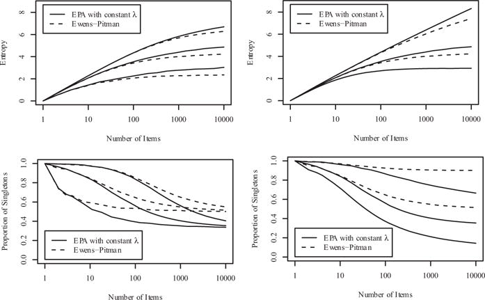
Top left panel: Mean entropy as a function of the number of items n (on the log scale), with discount parameter δ = 0.5 and mass parameter α = 1 (bottom), α = 10 (middle), and α = 100 (top). Top right panel: Same, with mass parameter α = 10 and discount parameter δ = 0 (bottom), δ = 0.5 (middle), and δ = 0.9 (top). Bottom panels show the mean proportion of subsets having only one item as a function of the number of items, using the same combinations of α and δ values. When δ = 0, the EPA distribution with constant similarity function). and the Ewens-Pitman distribution are the same.

For any mass parameter α and discount parameter δ, the probability of assigning to the new subset is the same for both our EPA distribution and the Ewens-Pitman distribution, regardless of the similarity function λ and the permutation σ used for our distribution. As such, the distribution of the number of subsets q_n in (5) and the mean in (6) apply to the Ewens-Pitman distribution, the two-parameter Chinese restaurant process, and the Pitman-Yor process (Teh 2006), just as they apply to our proposed EPA distribution. In summary, whereas the large sample behavior of the entropy and proportion of singletons differ, the distribution of the number of subsets is exactly the same. Therefore, the role of, interpretation of, and intuition regarding the mass parameter α and discount parameter δ regarding their influence on the number of subsets that one has for these established models carries over directly to the EPA distribution.

4.2. Comparison to Distance Dependent Chinese Restaurant Processes

Our EPA distribution resembles the distribution in the proceedings article of Dahl (2008) and the distance dependent Chinese restaurant process (ddCRP) of Blei and Frazier (2011). The key difference between our EPA distribution and these others is how they arrive at a distribution over partitions. The EPA distribution directly defines a distribution over partitions through sequential allocation of items to subsets in a partition. In contrast, both Dahl (2008) and Blei and Frazier (2011) define a distribution over a directed graph in which the n nodes have exactly one edge or loop, and the disjoint subgraphs form the subsets for the implied partition. There is a many-to-one mapping from these graphs to partitions and the probability of a given partition is implicitly defined by summing up the probabilities of graphs that map to the partition of interest. In the ddCRP distribution, the probability that item i has a directed edge to item j is proportional to λ(i, j) for j ≠ i and is proportional to α for j = i. The similarities may be zero and non symmetric. The probabilities of a directed edge for an item is independent of all other edges. Because of the asymmetry and the many-to-one nature, the probability of a directed edge from i to j is not the probability that items i and j are in the same subset of the partition.

The size of the set of graphs is nⁿ because each of the n items can be assigned to any one of the n items. Finding the probability for all possible graphs that map to a given partition π_n quickly becomes infeasible for moderately sized n and, thus, algorithms that require the evaluation of partition probabilities cannot be used. For example, although Blei and Frazier (2011) provide a Gibbs sampling algorithm for posterior inference in the ddCRP, it is not clear how to implement more general sampling strategies, for example, split-merge updates (Jain and Neal 2004,2007; Dahl 2003) which require evaluating the probability of a partition. In contrast, multivariate updating strategies can be applied to the EPA distribution because its p.m.f. for π_n is easily calculated. Bayesian inference also requires the ability to update other parameters (e.g., those of the sampling model) and hyperparameters (e.g., mass parameter α and the temperature τ). Standard MCMC update methods can be used for models involving the EPA distribution. In contrast, the ddCRP generally requires approximate inference for hyperparameters through Griddy Gibbs sampling (Ritter and Tanner 1992). Further, since the EPA distribution has an explicit p.m.f, the distribution of the number of subsets and its moments are available in closed form (Section 2.6), but this is not the case for the ddCRP. Computational issues aside, the ddCRP does not have a discount parameter 5 and thus does not have the same flexibility of the EPA distribution shown in Figure 4.

We illustrate stark differences between the EPA and ddCRP distributions using an example dataset in Section 6.1. There we show that, unlike the EPA distribution, the ddCRP has no clear separation between the mass parameter α and the similarity function λ in determining the number of subsets. As we will see, even though the two distributions make use of the same similarity information, they arrive at fundamentally different partition distributions.

4.3. Comparison to PPMx Model

Müller, Quintana, and Rosner (2011) proposed the PPMx model, a product partition model in which the prior partition distribution has the form: p(π_n|w₁,…, w_n) ∝ ${\displaystyle {\prod }_{j=1}^{qn}g\left({\mathbf{w}}^j\right)c\left(S_j\right)}$, where c(·) is a cohesion as in a standard product partition model, g(·) is a similarity function defined on a set of covariates, and w^j = {w_i : i ∈ S_j}. Although any cohesion may be used, the default is that of the Ewens distribution: c(S) = αΓ(|S|). If, in addition, g(·) is the marginal distribution from a probability model for the covariates, then the partition distribution p(π_n|w₁,…, w_n) is symmetric with respect to permutation of sample indices and is marginally invariant (as defined in Section 3.2). Müller, Quintana, and Rosner (2011) suggested default choices (depending on the type of the covariates) for the similarity function that guarantee these properties.

By way of comparison, our EPA distribution with a uniform prior of the permutation σ is also symmetric, but is not marginally invariant. On the other hand, the hyperparameters in the probability model on the covariates can heavily influence the partitioning process, but they are generally fixed in the PPMx model because posterior inference is complicated by an intractable normalizing constant. In contrast, posterior inference on hyperparameters in the EPA distribution is straightforward. As with the ddCRP but unlike our EPA distribution, the PPMx models does not have a clear separation between the mass parameter α and the covariates in determining the number of subsets. More generally, it is also not clear how to balance the relative effect of the covariates g(·) and the cohesion c(·) in the PPMx model. Finally, one can always define pairwise similarity information from item-specific covariates, but not all pairwise similarity information can be encoded as a function g(·) of item-specific covariates, as required by the PPMx model. As such, the EPA distribution can accommodate a wider class of information to influence partitioning.

5. Posterior Inference

In Bayesian analysis, interest lies in the posterior distribution of parameters given the data. The posterior distribution is not available in closed-form for the current approach, but a Markov chain Monte Carlo (MCMC) algorithm is available, as we now describe. This algorithm systematically updates parts of the parameter space at each iteration and performs many iterations to obtain samples from the posterior distribution.

First, consider the update of the partition π_n given the data y and all the other parameters. Because the model is not exchangeable, the algorithms of Neal (2000) for updating a partition π_n do not hold. As the p.m.f. is available, one could use a sampler that updates the allocation of many items simultaneously (e.g., a merge-split sampler (Jain and Neal 2004, 2007; Dahl 2003)). Here we use a Gibbs sampler (Gelfand and Smith 1990). To describe this sampler, suppose the current state of the partition is ${\pi }_n=\left\{S_1,\dots ,S_{q_n}\right\}$ and let $S_1^{-i},\dots ,S_{qn}^{-i}$ be these subsets without item i. Let ${\pi }_n^{i\to j}$ be the partition obtained by moving i from its current subset to the subset $S_j^{-i}$. Further, let ${\pi }_n^{i\to 0}$ denote the partition obtained by moving i from its current subset to an empty subset $S_0^{-i}$. The full conditional distribution for the allocation of item i is

$$p\left(i\in S_j^{-i}|\cdot \right)\propto p\left({\pi }_n^{i\to j}|\alpha ,\delta ,\lambda ,\sigma \right)p\left(y_i|{\varphi }_j\right)\text{for }j=0,1,\dots ,q_n,$$ (13)

where ϕ₀ is a new, independent draw from G₀ at each update. Note that $p\left({\pi }_n^{i\to j}|\alpha ,\delta ,\lambda ,\sigma \right)$ is calculated by evaluating (3) and (4) at the partition ${\pi }_n^{i\to j}$.

Because the p.m.f. of a partition π_n is easily calculated, standard MCMC schemes are available for updating other parameters, including α, δ, λ., σ, and $\varphi =\left({\varphi }_1,\dots ,{\varphi }_{q_n}\right)$. Herewemakea few notes. We suggest proposing a new permutation σ* by shuffing k randomly chosen integers in the current permutation σ, leaving the other n − k integers in their current positions. Being a symmetric proposal distribution, the proposed σ* is accepted with probability given by the minimum of 1 and the Metropolis ratio (p(π_n | α, δ, λ, σ*) p(σ*))/(p(π_n | α, δ, λ, σ) p(σ)), which reduces to p(π_n | α, δ, λ, σ*)/p(π_n | α, δ, λ, σ) when the prior permutation distribution p(σ) is uniform. As k controls the amount of change from the current permutation σ, the acceptance rate tends to decrease as k increases. If the similarity function λ involves hyperparameters, such as a temperature τ, a Gaussian random walk is a natural sampler to use. Likewise, a Gaussian random walk can be used to update the mass parameter α and the discount parameter δ. When δ = 0, the distribution of the number of subsets is the same as in Dirichlet process mixture models and, as such, the Gibbs sampler of Escobar and West (1995) for updating the mass parameter α also applies to the EPA distribution.

Now consider updating $\varphi =\left({\varphi }_1,\dots ,{\varphi }_{q_n}\right)$ given the data and the other parameters. This update is the same as in any other random partition model. For j = 1, …, q_n, update ϕ_j using its full conditional distribution

$$p\left({\varphi }_j|y_i:i\in S_j\right)\propto p\left({\varphi }_j\right){\displaystyle \prod _{i\in S_j}p\left(y_i|{\varphi }_j\right),}$$

where p(ϕ) is the density of the centering distribution G₀. This full conditional distribution can usually be sampled directly if G₀ is conjugate to the sampling model p(y | ϕ). If not, any other valid MCMC update can be used, including a Metropolis-Hastings update.

Finally, we consider a sampling scheme for the estimation of p(y_n+1 | y₁,…,y_n), the density of a new observation y_n+1 whose similarities λ(n + 1, j) are available for j = 1, …, n. Pick an initial valuey_n+1. Use the posterior sampling procedure as described previously but also update the value of y_n+1 at each iteration by sampling y_n+1 using the current value of its model parameter θ_n+1. Let ${\theta }_{n+1}^{\left(b\right)}$ denote the value of this model parameter for the observation y_n+1 at iteration b. Under squared error loss, the Bayes estimate of p(y_n+1 | y₁, …, y_n) based on B samples from the MCMC scheme is ${\displaystyle {\sum }_{b=1}^{B}p\left(y_{n+1}|{\theta }_{n+1}^{\left(b\right)}\right)/B.}$.

6. Demonstrations

6.1. Arrests Dataset

In this section, we illustrate properties of the EPA distribution and compare its behavior to the ddCRP of Blei and Frazier (2011) using the “USArrests” dataset in R. We see that the two distributions use the same similarity information to arrive at fundamentally different partition distributions. As the temperature τ increases, the EPA distribution smoothly moves away from the Ewens distribution, placing more probability on partitions that group items with small distances (and that separate those with large distances), yet keeping the total probability of partitions with a given number of subsets constant. In contrast, the ddCRP does not correspond to the Ewens when τ = 0 and, as temperature goes to infinity, it collapses all probability to the partition with each item in its own singleton subset.

The “USArrests” dataset contains statistics on “arrests per 100,000 residents for assault, murder, and rape in each of the 50 United States in 1973” and “the percent of the population living in urban areas.” The Euclidean distances between the four-dimensional standardized data vectors of n = 5 selected states are used. For both distributions, we use the exponential similarity function λ(i, j) = f(d_ij) = exp(−τd_ij) and let α = 2. In addition, for the EPA distribution, let δ = 0 and p(σ) = 1/n!. We compute the probability of each of the B(5) = 52 possible partitions of the five states for a range of temperatures.

The evolution — as temperature x increases — of the probabilities of the 52 partitions are displayed in the left panel of Figure 5. The cumulative probabilities of the partitions for the five states are displayed horizontally, and the ordering of the partitions is consistent across temperatures. For each partition, the cumulative probabilities across temperatures are joined to form the curves and the probability of a given partition is the difference between curves. The curves of several interesting partitions are identified with capital letters. Temperature x = 0 corresponds to the partition distribution of the Ewens distribution since λ(i, j) is constant when τ = 0. As the temperature increases, the pairwise distances become more influential and eventually the EPA distribution has appreciable probability on several partitions and virtually no probability for others. For example, whereas the partition “J” in Figure 5 has probability about 0.01 when τ = 0 (corresponding to the Ewens distribution), it grows about 10 fold in probability when τ = 4 because this partition matches well the pairwise distance information. Therefore, in the EPA distribution, the temperature x controls the degree to which the prior distance information influences the partition distribution. The left panel of Figure 5 also shows that the aggregate probability for partitions with 1, 2, 3, 4, and 5 subsets is constant across temperature, illustrating a key feature of the EPA distribution discussed in Section 3.1: Our distribution allocates probability among partitions within a given number of subsets, but it does not shift probability among sets of partitions with different numbers of subsets.

Figure 5.

The cumulative probabilities of the 52 partitions for the five states selected from the “USArrests”dataset for the EPA distribution (left) and the ddCRP (right). For each partition, the cumulative probabilities across temperatures are joined to form the curves and the probability of a given partition is the difference between curves. Capital letters label the same partitions for both the left- and right-hand sides.

The right-hand side of Figure 5 is the same plot for the ddCRP using the same value for mass parameter α, the same distance information d_ij, and the same similarity function λ(i, j) = f(d_ij) = exp(−τd_ij). Capital letters label the same partitions for both the left- and right-hand sides of the figure. In contrast with the EPA distribution, the ddCRP: (i) does not correspond to the Ewens distribution with τ = 0, (ii) the distribution of the number of subsets is heavily influenced by the temperature τ, and (iii) partition ‘K’ initially dominates but partition ‘A’ eventually absorbs all the probability mass when τ → ∞. We thus see that, even with the same inputs, the EPA and ddCRP have fundamentally different properties and our EPA distribution adds to the set of available prior distributions that one can choose.

6.2. Bayesian Density Estimation for Dihedral Angles

We now demonstrate the EPA distribution as a prior partition distribution in Bayesian density estimation for protein structure prediction and find that using the EPA distribution significantly improves prediction over competing methods. A protein is a string of amino acids that together adopt unique three-dimensional conformations (i.e., structures) to allow the protein to carry out its biochemical function. While it is relatively easy to determine the amino acid sequence of the protein, solving its structure is more challenging. A proteins structure can largely be characterized by the (ϕ, ψ) torsion angles at each amino acid position. The task of protein structure prediction is simplified if, for a given protein family, the distribution of (ϕ, ψ) angles at each position can be estimated. The sine model (Singh, Hnizdo, and Demchuk 2002) of the bivariate von Mises distribution is a model for (ϕ, ψ) angles

$$p\left(\left(\varphi ,\psi \right)|\mu ,\nu ,{\kappa }_1,{\kappa }_2,\lambda \right)=C\text{exp}\left\{{\kappa }_1\text{cos}\left(\varphi -\mu \right)+{\kappa }_2\text{cos }\left(\psi -\nu \right)+\lambda \text{sin}\left(\varphi -\mu \right)\text{sin }\left(\psi -\nu \right)\right\},$$

where $C^{-1}=4{\pi }^2{\displaystyle {\sum }_{m=0}^{\infty }\left(\frac{2m}{m}\right){\left(\frac{{\lambda }^2}{4{\kappa }_1{\kappa }_2}\right)}^m{I}_m\left({\kappa }_1\right)I_m\left({\kappa }_2\right)}$, ϕ, ψ, μ, ν ∈ (−π, π], κ₁, κ₂ > 0, and λ ∈ (−∞, ∞). Note that I_m(x) is the modified Bessel function of the first kind of order m. Lennox et al. (2009) used the sine model as a kernel in a Dirichlet process mixture model for nonparametric density estimation of a (ϕ, ψ) distribution. In the notation of (2), y_i = (ϕ_i, ψ_i) and θ_i = (μ_i, ν_i, κ_1i, κ_2i, λ_i). For the centering distribution G₀, we use the product of a bivariate uniform distribution on (−π, π] × (−π, π] (for μ, ν) and a bivariate Wishart distribution with shape 2 and rate matrix 0.25 I₂ (for κ₁, κ₂, λ), where I₂ is the 2 × 2 identity matrix and the mean is therefore 0.5 I₂.

In this demonstration, our data are (ϕ, ψ) angles for 94 members of the globin family at aligned positions 93,94,95,104, 105, and 106, based on the default multiple sequence alignment from MUSCLE 3.8.31 (Edgar 2004). While Lennox et al. (2009) models the (ϕ, ψ) distribution of a protein at a specific position based on angular data, their use of the Ewens distribution for the prior partition distribution p(π_n) does not take advantage of the known amino acid sequence of the protein of interest. Here we replace the Ewens distribution with several specifications of our EPA distribution, the PPMx model, and a simple data-subsetting approach, all of which use the known amino acid sequence. Thus we mimic the task of protein structure prediction by using amino acid sequences to inform a prior partition distribution, resulting in density estimates tailored to a specific protein.

For each model described below, 20 independent Markov chains were run using the MCMC sampling algorithm described in Section 5 with 27,500 scans, discarding the first 2500 as burn-in and applying 1-in-5 thinning. Half of the 20 chains were initialized with a partition having all observations in their own subsets and the other half were initialized with all observations in the same subset. For each model and position, we compute the log pseudo marginal likelihood (LPML), that is, the sum of conditional predictive ordinates (Geisser and Eddy 1979; Gelfand 1996) across the 94 proteins. This evaluation criterion employs leave-one-out cross-validation to compare the predicted densities to the actual observed angle pairs. All comparisons are relative to the model using the Ewens prior partition distribution with mass parameter α fixed at 1.0. Table 1 provides the difference between the mean LPML values for each model discussed below and the baseline model using the Ewens prior partition distribution. Large positive values in the table indicate better fit to the data, with differences larger than a few units generally being statistically significant.

Table 1.

Differences in the log pseudo marginal likelihood (LPML) between several models and the model using the standard Ewens distribution.

	Position
	93	94	95	104	105	106	Total
1. Ewens	0.0	0.0	0.0	0.0	0.0	0.0	0.0
2. EPA using BLAST similarity	28.0	40.3	51.3	− 0.8	− 0.1	57.9	176.6
3. EPA using 7-covariates similarity	27.8	31.8	45.1	− 0.3	− 0.6	57.5	1612
4. EPA using 1-covariate similarity	27.9	17.0	26.7	0.6	−1.3	22.3	93.3
5. PPMx using 7-covariates similarity	− 54.6	− 30.5	7.1	− 45.9	−18.63	− 8.6	− 1335
6. PPMx using 1-covariate similarity	24.3	10.7	15.6	− 4.2	− 5.9	17.3	57.7
7. Ewens w/ BLAST subsetting, t = 15	2.7	5.1	15.4	− 0.4	1.8	6.2	30.8
8. Ewens w/ BLAST subsetting, t = 25	3.8	5.9	29.5	− 4.7	− 05	17.7	515
9. Ewens w/ BLAST subsetting, t = 35	−19.6	− 1.8	31.7	− 26.0	− 205	6.9	− 292

NOTE: Large positive values indicate better fit.

Our baseline specification of the EPA distribution has similarity function λ(i, j) being one plus the mean BLAST bit score between the amino acid sequences for proteins i and j. A BLAST bit score is a pairwise measure of similarity between two proteins. It is large for a pair of proteins having similar amino acid sequences and small otherwise. Twenty-seven percent of the similarities are 1 and the remaining have a five-number summary of (9, 32, 55, 110, 306). The temperature τ has a Gamma (2, 0.5) prior (with mean 4) and we use a uniform prior on the permutation σ. We fix the discount δ at 0.0 and, as with the Ewens distribution, the mass parameter α is fixed at 1.0. When updating the permutation σ, the sampling algorithm proposes to update k = 46 items and the mean acceptance rate is about 30%. When updating the temperature τ, a Gaussian random walk proposal is used with standard deviation 2.0 and the mean acceptance rate is 59%. Diagnostics indicate that the Markov chains mix well. The LPML results for this model are found in row 2 of Table 1. There is substantial improvement at all the positions except positions 104 and 105. At these positions, the performance is about that of the Ewens distribution because the (ϕ, ψ) distributions are highly concentrated in one region and, therefore, the amino acid sequence information is not helpful in prediction.

The BLAST bit scores are not compatible with the recommended similarity functions for the PPMx model because they are not individual-specific covariates, but rather a measure of similarity between two proteins. It is therefore not obvious how to incorporate them in the PPMx framework. We can, however, treat the the amino acids at positions 93, 94, 95, 99, 104, 105, and 106 as seven categorical covariates, taking one of 21 values (representing missingness or one of the 20 amino acids). We use the default Dirichlet-multinomial similarity function and follow the recommendation for setting the Dirichlet hyperparameters less than one. (Specifically, we set them at 0.5.) For the sake of comparison, we use Monte Carlo simulation from the prior to find a value for the mass parameter α such that the prior number of subsets is the same as that obtained by using the Ewens or EPA distribution with α = 1. The results are found in row 5 of Table 1 and show that, for most positions, the PPMx model performs substantially worse than the Ewens distribution. We caution, however, that many of the Markov chains exhibit poor mixing. We also find poor performance with smaller values for the mass parameter α or when substantially increasing the burn-in period (not shown). We suspect that this PPMx prior has several local modes that dominate the likelihood. To make a direct comparison, we also consider an alternative specification of the EPA prior partition distribution where the similarity function λ(i, j) is one plus the number of times proteins i and j share the same value across these seven covariates. We find that this second specification of EPA (row 3) performs substantially better than the PPMx for these same covariates (row 5) and almost as well as the original EPA specification (row 2).

We suspect that other formulations of the PPMx model may perform better. Indeed, consider the PPMx model using the default Dirichlet-multinomial similarity function based only on the amino acid at the current position. Under this formulation the PPMx model (row 6 of Table 1) performs much better than the Ewens distribution (row 1) overall. By way of comparison, consider the EPA distribution where the similarity function λ(i, j) is 2 if proteins i and j have the same amino acid at that position and is 1 otherwise. This EPA formulation (row 4) also performs much better than the Ewens distribution (row 1) and dominates the analogous PPMx formulation (row 6) at each position. While the EPA distribution dominates the PPMx distribution in this case, we suspect it may perform better in other scenarios or with non-default choices for the PPMx similarity function.

The EPA distribution allows pairwise similarity information to inform the partitioning. An ad hoc method capturing this idea uses the standard Ewens distribution but subset the data to only include those observations whose similarities to the observation of interest exceed a threshold. The subsetting threshold is analogous to the temperature τ in the EPA distribution, but there the temperature τ can be treated as random with a prior distribution whereas the threshold must be fixed to implement the subsetting approach. Further, discarding observations will likely lead to a loss of precision in estimating other parameters. We examine several thresholds for the BLAST bit scores and the results for the best thresholds are found on rows 7–9 in Table 1. For threshold t = 15 and t = 25, subsetting is usually better than not subsetting (row 1), but the PPMx model (row 6) and EPA distribution (rows 2–4) perform better.

Finally, we consider posterior inference on the hyperparameters. Let the discount 5 have a mixture prior distribution with a point-mass at 0 with probability 0.5 and a Beta(1, 3) distribution otherwise. We again run 20 independent Markov chains for each position (but do not leave out an observation). Whereas the prior probability that δ = 0 is 0.5, the posterior probabilities at positions 93, 94, 95, 104, 105, and 106 are 0.47, 0.36, 0.38, 0.53, 0.51, and 0.58, respectively (all of which are statistically different from 0.5). The posterior expectations of temperature x are 3.3, 10.4, 7.8, 4.1, 3.4, and 6.9, respectively (all of which are statistically different from the prior expectation of 4). To assess the posterior learning on the permutation σ, consider the indices of observations in σ. The uniform prior of σ makes the prior expectation of an index be 94/2 = 47 for all 94 observations. The five-number summary of the posterior means of the indices at position 94 is (11.6, 48.0, 48.9, 50.0, 57.7) and this pattern is consistent across independent Markov chains. At position 106, the five-number summary is (31.5, 46.9, 49.4, 51.2, 53.4). We conclude that, in some cases, there is substantial learning on these parameters whereas, in other cases, there is little difference between the prior and posterior distributions.

6.3. Bayesian Linear Regression with Latent Clusters

Section 6.2 demonstrates our proposed distribution in an application with 94 observations and five parameters per subset. To see how our proposal performs as the dimension and sample size grow, we now consider a simulation study with n = 1050 observations and 31 parameters per subset. Consider a linear regression model in which a response y_i has a normal distribution with mean x_iβ_i and precision λ_i, for covariates x_i = (x_i1,…, x_ip), i = 1, …, n, and p = 30. In this simulation study, the data are generated from one of three sets of regression coefficient vectors and precisions. The inferential goal is to estimate the latent partition π and the regression coefficient vectors β₁, …, β_n. To aid in estimation, partition covariates are available as prior information to help separate the data into subsets.

The specifics of the data generation are as follows: Set x_i1 = 1 and sample all the other x’s from the uniform distribution of the unit interval. For i ∈ S₁ = {1,…, 350}, set (β_i, λ_i) to be ϕ₁ = ((0, …,0), 1.0). For i ∈ S₂ = {351,…, 700}, set (β_i, λ_i) to be a tuple ϕ₂ containing: (i) a column vector whose first 10 elements are 0.9 and the other elements are 0 and (ii) 1.0. For i ∈ S₃ = {701, …, 1050}, set (β_i, λ) to be a tuple ϕ₃ containing: (i) a column vector ϕ₃ whose first 6 elements are 1.0 and the other elements are 0, and (ii) 1.0. Partition covariates w₁, …, w_n are sampled from one of three four-dimensional multivariate normal distributions, depending on the subset to which i belongs. The parameters are taken from the empirical moments of the three classes in the iris data (Fisher 1936), with the first, second, and third subsets corresponding to “setosa,” “versicolor,” and “virginica,” respectively. Note that subsets 2 and 3 have similar coeicients and their observations have partition covariates drawn from somewhat overlapping distributions.

In the notation of (2), we wish to estimate the parameters π_n = {S₁, S₂, S₃} and ϕ = ((ϕ₁, ϕ₂, ϕ₃). The prior distribution for the ϕ’s is the conjugate multivariate normal-gamma distribution Ng(β, λ | μ, Λ, α, β) where μ = 0, Λ is the identity matrix, α = 1, and β = 1. Three prior distributions for the partition π_n are considered and the resulting performance is compared. First, we consider the Ewens distribution which ignores the partition covariates w’s. Second, we consider the PPMx model (Müller, Quintana, and Rosner 2011) using their default formulation of the similarity function based on the centered and scaled versions of the w’s. Finally, we consider our EPA distribution using an exponential similarity function applied to the Euclidean distance between the w’s. We place a uniform prior on the permutation σ and the temperature x has a Gamma(2, 0.5) prior (with mean 4). The discount 5 is fixed at 0.0. We set the mass parameter α to 1.0 for the Ewens and EPA distributions and to 23.0 for the PPMx model, making the prior expected number of subsets to be approximately 7.5 for all three distributions.

Thirty independent Markov chains are run for 2000 iterations for each of the three models using our software written in Scala. The frst 500 iterations are discarded as burn-in. The performance of the models is assessed using Monte Carlo estimates of the posterior mean of the adjusted Rand index (ARI) (Hubert and Arabie 1985) with respect to the true partition. The ARI is a measure of similarity between two partitions, with 1.0 corresponding to perfect agreement. The mean ARI is 0.227, 0.505, 0.648 for the models using the Ewens, PPMx, and EPA distributions, respectively. We also compute the posterior mean of the sum of squared Euclidean distances from the true coefcient vectors and find values 8.68, 4.24, and 3.91 for the models using the Ewens, PPMx, and EPA distributions, respectively. All pairwise differences are statistically significant (p-value less than 0.01) based on a two-sample t-test. Using either evaluation criteria, the model with the EPA distribution performs the best in this simulation study and demonstrates the viability of the EPA distributions in high dimensions. The PPMx model, which also performs well, has the advantage that it runs in about 59% of the CPU time required for the EPA distribution.

7. Conclusion

Our proposed EPA distribution uses pairwise similarity information to define a random partition distribution. A key feature of our formulation is that probability is allocated among partitions within a given number of subsets, but probability is not shifted among sets of partitions with different numbers of subsets. This feature provides a clear separation of the roles of: (i) the mass parameter α and discount parameter 5 and (ii) the pairwise similarity function λ and permutation σ. Further, the distribution of the number of subsets is unchanged from the usual Ewens and Ewens-Pitman distributions, and the intuition one has regarding the α and δ from these familiar distributions carries over. We note that our distribution is invariant to scale changes in the similarity λ, which aligns with the idea that similarity is a relative rather than an absolute concept. Our formulation also has an explicit p.m.f. with an easily-evaluated normalizing constant, so standard MCMC samplers are available for posterior inference on the partition and hyperparameters influencing the partition distribution.

It could be argued that our proposal excessively shrinks toward the Ewens and Ewens-Pitman distributions and that the distribution of the number of subsets should be influenced by the similarity information. In a preliminary formulation, we initially considered defining Pr(σ_t ∈ S | α, δ, λ, π(σ₁, …, σ_t−1)) in (4) to be proportional to ${\displaystyle {\sum }_{{\sigma }_s\in S}\lambda \left({\sigma }_t,{\sigma }_s\right)}-\delta$ for an existing subset S and proportional to α + δq_t−1 for a new subset. This makes the probability of forming a new subset depend on the similarity function and, therefore, the distribution of the number of subsets different from that of the Ewens, Ewens-Pitman, and EPA distributions. We chose to not pursue this formulation for a few reasons. First, the normalizing constant of the p.m.f. would then become intractable, making posterior inference difficult for the partition and hyperparameters. Second, we feel that the clear separation of the roles of the α, δ, and λ can be desirable and a feature that distinguishes our distribution from the PPMx and ddCRP distributions. We view our contribution as expanding the choices available for flexible Bayesian modeling. Finally, we showed in the demonstrations of Sections 6.2 and 6.3 that using the EPA distribution as a prior partition distribution can provide better statistical performance.

References

- Airoldi EM, Costa T, Bassetti F, Leisen F, Guindani M. Generalized Species Sampling Priors With Latent Beta Reinforcements. Journal of the American Statistical Association. 2014;109:1466–1480. doi: 10.1080/01621459.2014.950735. [DOI] [PMC free article] [PubMed] [Google Scholar]
- Aldous D, Ibragimov I, Jacod J, Aldous D. cole d’t de Probabilits de Saint-Flour XIII 1983, vol. 1117 of Lecture Notes in Mathematics. Berlin / Heidelberg: Springer; 1985. Exchangeability and Related Topics; pp. 1–198. [Google Scholar]
- Antoniak CE. Mixtures of Dirichlet Processes With Applications to Bayesian Nonparametric Problems. The Annals of Statistics. 1974;2:1152–1174. [Google Scholar]
- Arratia R, Barbour AD, Tavaré S. Logarithmic Combinatorial Structures: A Probalistic Approach. Zurich: European Mathematical Society; 2003. [Google Scholar]
- Bell ET. Exponential Numbers. American Mathematical Monthly. 1934;41:411–419. [Google Scholar]
- Blei DM, Frazier PI. Distance Dependent Chinese Restaurant Processes. Journal of Machine Learning Research. 2011;12:2461–2488. [Google Scholar]
- Dahl DB. An Improved Merge-Split Sampler for Conjugate Dirichlet Process Mixture Models. University of Wisconsin - Madison, Department of Statistics; 2003. (Technical Report 1086). [Google Scholar]
- Dahl DB. JSM Proceedings, Section on Bayesian Statistical Science. Alexandria, VA: American Statistical Association; 2008. Distance-Based Probability Distribution for Set Partitions With Applications to Bayesian Nonparametrics. [Google Scholar]
- De Blasi P, Favaro S, Lijoi A, Mena R, Prunster I, Ruggiero M. Are Gibbs-Type Priors the Most Natural Generalization of the Dirichlet Process? Pattern Analysis and Machine Intelligence, IEEE Transactions on. 2015;37:212–229. doi: 10.1109/TPAMI.2013.217. [DOI] [PubMed] [Google Scholar]
- Edgar RC. MUSCLE: Multiple Sequence Alignment With High Accuracy and High Throughput. Nucleic Acids Research. 2004;32:1792–1797. doi: 10.1093/nar/gkh340. [DOI] [PMC free article] [PubMed] [Google Scholar]
- Escobar MD, West M. Bayesian Density Estimation and Inference Using Mixtures. Journal of the American Statistical Association. 1995;90:577–588. [Google Scholar]
- Ewens W. The Sampling Theory of Selectively Neutral Alleles. Theoretical Population Biology. 1972;3:87–112. doi: 10.1016/0040-5809(72)90035-4. [DOI] [PubMed] [Google Scholar]
- Ferguson TS. A Bayesian Analysis of Some Nonparametric Problems. The Annals of Statistics. 1973;1:209–230. [Google Scholar]
- Fisher RA. The Use of Multiple Measurements in Taxonomic Problems. Annals of Eugenics. 1936;7:179–188. [Google Scholar]
- Geisser S, Eddy WF. A Predictive Approach to Model Selection. Journal of the American Statistical Association. 1979;74:153–160. [Google Scholar]
- Gelfand AE. Empirical Bayes Methods for Combining Likelihoods: Comment. Journal of the American Statistical Association. 1996;91:551–552. [Google Scholar]
- Gelfand AE, Smith AFM. Sampling-Based Approaches to Calculating Marginal Densities. Journal of the American Statistical Association. 1990;85:398–409. [Google Scholar]
- Hubert L, Arabie P. Comparing Partitions. Journal of Classification. 1985;2:193–218. [Google Scholar]
- Jain S, Neal RM. A Split-Merge Markov Chain Monte Carlo Procedure for the Dirichlet Process Mixture Model. Journal of Computational and Graphical Statistics. 2004;13:158–182. [Google Scholar]
- Jain S, Neal RM. Splitting and Merging Components of a Nonconjugate Dirichlet Process Mixture Model. Bayesian Analysis. 2007;2:445–472. [Google Scholar]
- Lau JW, Green PJ. Bayesian Model Based Clustering Procedures. Journal of Computational and Graphical Statistics. 2007;16:526–558. [Google Scholar]
- Lee J, Quintana FA, Müller P, Trippa L. Defining Predictive Probability Functions for Species Sampling Models. Statistical Science. 2013;28:209–222. doi: 10.1214/12-sts407. [DOI] [PMC free article] [PubMed] [Google Scholar]
- Lennox KP, Dahl DB, Vannucci M, Tsai JW. Density Estimation for Protein Conformation Angles Using a Bivariate von Mises Distribution and Bayesian Nonparametrics. Journal of the American Statistical Association. 2009;104:586–596. doi: 10.1198/jasa.2009.0024. [DOI] [PMC free article] [PubMed] [Google Scholar]
- Müller P, Quintana F, Rosner GL. A Product Partition Model With Regression on Covariates. Journal of Computational and Graphical Statistics. 2011;20:260–278. doi: 10.1198/jcgs.2011.09066. [DOI] [PMC free article] [PubMed] [Google Scholar]
- Neal RM. Markov Chain Sampling Methods for Dirichlet Process Mixture Models. Journal of Computational and Graphical Statistics. 2000;9:249–265. [Google Scholar]
- Park JH, Dunson DB. Bayesian Generalized Product Partition Model. Statistica Sinica. 2010;20:1203–1226. [Google Scholar]
- Pitman J. Exchangeable and Partially Exchangeable Random Partitions. Probability Theory and Related Fields. 1995;102:145–158. [Google Scholar]
- Pitman J. Some Developments of the Blackwell-MacQueen Urn Scheme. In: Ferguson TS, Shapley LS, MacQueen JB, editors. Statistics, Probability and Game Theory. Vol. 30. Beachwood, OH: Institute of Mathematical Statistics; 1996. pp. 245–267. (IMS Lecture Notes Monograph Series). [Google Scholar]
- Pitman J, Yor M. The Two-Parameter Poisson-Dirichlet Distribution Derived from a Stable Subordinator. The Annals of Probability. 1997;25:855–900. [Google Scholar]
- Quintana FA. A Predictive View of Bayesian Clustering. Journal of Statistical Planning and Inference. 2006;136:2407–2429. [Google Scholar]
- Ritter C, Tanner MA. Facilitating the Gibbs Sampler: The Gibbs Stopper and the Griddy-Gibbs Sampler. Journal of the American Statistical Association. 1992;87:861–868. [Google Scholar]
- Shahbaba B, Neal RM. Nonlinear Models Using Dirichlet Process Mixtures. Journal of Machine Learning Research. 2009;10:1829–1850. [Google Scholar]
- Singh H, Hnizdo V, Demchuk E. Probabilistic Model for Two Dependent Circular Variables. Biometrika. 2002;89:719–723. [Google Scholar]
- Teh YW. A Hierarchical Bayesian Language Model Based on Pitman-Yor Processes; Proceedings of the 21st International Conference on Computational Linguistics and 44th Annual Meeting of the Association for Computational Linguistics; Sydney, Australia. Stroudsburg, PA: Association for Computational Linguistics; 2006. pp. 985–992. [Google Scholar]