Multiscale Network Representation of Physiological Time Series for Early Prediction of Sepsis

Abstract

Sepsis, a dysregulated immune-mediated host response to infection, is the leading cause of morbidity and mortality in critically ill patients. Indices of heart rate variability and complexity (such as entropy) have been proposed as surrogate markers of neuro-immune system dysregulation with diseases such as sepsis. However, these indices only provide an average, one dimensional description of complex neuro-physiological interactions. We propose a novel multiscale network construction and analysis method for multivariate physiological time series, and demonstrate its utility for early prediction of sepsis. We show that features derived from a multiscale heart rate and blood pressure time series network provide approximately 20% improvement in the area under the receiver operating characteristic (AUROC) for four hours ahead prediction of sepsis over traditional indices of heart rate entropy (0.78 versus 0.66). Our results indicate that this improvement is attributable to both the improved network construction method proposed here, as well as the information embedded in the higher order interaction of heart rate and blood pressure time series dynamics. Our final model, which included the most commonly available clinical measurements in patients’ Electronic Medical Records, multiscale entropy features as well as the proposed network-based features, achieved an AUROC of 0.80. Prediction of the onset of sepsis prior to clinical recognition will allow for meaningful earlier interventions (e.g., antibiotic and fluid administration), which have the potential to decrease sepsis-related morbidity, mortality and healthcare costs.

1. Introduction

Sepsis is a significant healthcare burden with high morbidity and mortality among Intensive Care Unit (ICU) patients. Prompt recognition and treatment are central to optimizing outcomes, yet antecedent signs and symptoms of sepsis can be subtle and unrecognized by clinicians despite continuous patient monitoring.

In recent years, Machine learning-based predictive algorithms for early prediction of septic shock have been proposed (Henry et al. 2015; Ghosh et al. 2017) with AUROC values in the range of 0.80–0.85. However, hemodynamic management through fluid and pressors administration are the only available intervention in septic patients at risk for shock, with a recent study suggesting that such interventions may not be associated with lower in-hospital mortality (Seymour et al. 2017).

Using a machine learning-based algorithm to predict sepsis with enough lead-time could prevent its occurrence in those deemed high risk if antibiotics are initiated before sepsis onset. Desautels and colleagues used a proprietary machine learning algorithm with commonly available clinical measurements in an Electronic Medical Record (EMR) to predict sepsis four hours before it occurred (Desautels et al. 2016), however, prediction of sepsis has proved to be difficult (AUROC 0.74). This may be partially due to the fact that early prediction of sepsis requires up-to-date clinical measurements, which are more likely to be available if there is already a clinical suspicion of infection (as in the case of septic shock prediction). Even when up-to-date clinical measurements are available, such data tends to have a low temporal resolution (once every 30 minutes or lower) and is subjected to recall and information bias. For instance, blood pressure documentation by bedside clinicians can be biased towards normal when compared to corresponding blood pressure waveforms (Hug et al. 2011), in part due to back-documentation of past data. However, incorporation of continuous high-resolution data (such as second-by-second vital signs time series from the bedside monitors) has the potential to mitigate the aforementioned problems and provide a more timely prediction of sepsis.

Sepsis is known as a dysregulated immune-mediated host response to infection. Alteration in heart rate (HR) and blood pressure (BP) variability and coupling prior to onset of sepsis has been reported in the literature (Buchman 2004, Moorman et al. 2011), and potential links to neuro-immune system interactions have been established. According to the anti-inflammatory reflex model (Huston et al. 2011), pathogen-induced inflammation increases the activity of vagus nerve which controls the production of proinflammatory cytokines and prevents tissue damage. Although, the relationship amongst inflammation, vagus nerve activity and heart rate variability (HRV) and Baroreflex control of BP and HR is complex, this model suggests that monitoring indices of heart rate variability and complexity (as markers of vagus nerve activity) may provide useful surrogate markers of the inflammatory reflexes in health and disease.

Entropy is a measure of unpredictability of the state of a system, or equivalently, of its average information content. Information can be thought of as a measure of surprise and entropy can be thought of as a measure of average surprise. In recent years, one of the novel advances in time series representation and quantification has been the mapping of time series to network, based on ideas such as transition probabilities (Campanharo et al. 2011, Nicolis et al. 2005), visibility (Lacasa et al. 2015, Luque et al. 2009), and correlations (Steinhauser et al. 2008, Yang et al. 2008). Each of these studies demonstrated that many characteristics of time series can be extracted from the properties of the corresponding network. Moreover, network-based representations are capable of extracting more nuanced characteristics of time series.

In particular, the concept of modularity has been used to characterize time series (Sun et al. 2007). By modularity, we mean a set of densely connected nodes within a network. Other authors have used the terms “cluster” or “communities” (Girvan et al. 2002, Duch et al. 2005, Fortunato 2010) to denote such constellation of nodes. Networks with high modularity have dense connections between the nodes within modules, but sparse connections between nodes in different modules. An interpretation of what these modules represent is in terms of “set points” of a system. Classical physiology is grounded on the principle of homeostasis in which regulatory mechanisms act to maintain a steady state, i.e., “set point”. However, as argued by Ary Goldberger et al. in his editorial (Goldberger 2001), many physiological systems tend to operate out of equilibrium and in locally stable regimes (several set points versus a single set point), hence the observation of modularity in the resulting networks of joint HR and BP time series.

Therefore an aim of this study was to investigate the connection between HR and BP time series structure, as captured through quantification of the structure of their corresponding network representation, and early signs of sepsis. However, physiological time series can often exhibit complex patterns of variability over multiple time scales (Ivanov et al. 1999, Costa et al. 2002). For instance, time series of BP can exhibit oscillations on the order of seconds (e.g., due to the variations in sympathovagal balance), to minutes (e.g., as a consequence of fever, blood loss, or behavioral factors), to hours (e.g., due to humoral variations, sleep-wake cycle, or circadian effects) (Mancia 2012; Parati et al. 2015). It should also be noted that interactions (or coupling) between physiological systems are often caused by distinct physiological mechanisms that operate across different time scales (Bartsch et al. 2014). We therefore investigate the multiscale structure of vital signs network and their utility for early prediction of sepsis.

2. Materials and Methods

This section describes the dataset used, as well as the proposed algorithm for prediction of sepsis, and the evaluation methods. All data processing, creation of networks, feature extraction, and classifier training and testing were performed using Matlab R2016b (MATLAB 2016).

2.1. Dataset

Heart rate (HR) and mean arterial blood pressure (MAP) time series at 2 seconds resolution were collected from bedside monitors in an Emory affiliated ICU, using the BedMaster system (Excel Medical Electronics, Jupiter FL, USA); a third-party software connected to the hospitals General Electric (GE) monitors for the purpose of electronic data extraction and storage of high resolution waveforms. All adult ICU units were included in this study, including Medical and Surgical, Cardiac Care, and Neuro-intensive care units. The bedside monitor data was then matched and time synchronized to each patients EMR data. A total of 100 patients (22%) met the definition of sepsis by Seymour et al. 2016 at some time point during their ICU stay. Specifically, all episodes of suspected infection (t_suspicion) were identified as the earlier timestamp of antibiotics and blood cultures within a specific time span; if the antibiotic was given first, the culture sampling must have been obtained within 24 hours. If the culture sampling was first, the antibiotic must have been ordered within 72 hours. The onset time of sepsis (t_sepsis) was then defined as an episode of suspected infection with a two or more points change in the Sequential Organ Failure Assessment (SOFA) score from up to 48 hours before to up to 24 hours after the t_suspicion. The average length of hospital stay (LOS) among the septic patients was 137.6 [68.2–295.7] hours, and the percentages of in-hospital mortality and in-patient hospice were 15.2% and 13.5%, respectively. The septic patients exhibited a higher average SOFA score compared to non-septic patients (4.8 [3.1–6.8] versus 1.6 [0.6–3.4]).

2.2. Model

Our goal is to define a set of physiological states, that are represented by the nodes of a network. Transition among these physiological states are captured by the network edges, and therefore the network structure would capture the state trajectory through time.

Dynamic Bayesian networks have been used to model the trajectory of the state of physiological systems (Lehman et al. 2015), where a system’s state refers to a set of (observed or latent) attributes of the system that summarize all one needs to know about the system to predict its evolution through time (Buchman 1996). Parametric approaches such as the switching dynamical systems (Quinn et al. 2009) assume the states transition dynamics to follow a Markov Chain. The approach taken in this work is non-parametric and extracts a set of system states via adaptive partitioning of the state-space. The partitions define the nodes in the corresponding network representation of the time series, and the transition probabilities are captured by the edges.

2.2.1. Defining the state-space

Time-lagged embedding provides information on the underlying dynamical system without having direct access to all the system variables (Takens et al. 1981). As a first step to defining the state-space we applied timed-lagged embedding (of order l) to each time series dimensions. Next, the embedded time series samples were replaced by their rank orders (via rank order transformation) to achieve robustness to outliers. This step exploited the fact that mutual information between a set of random variables is invariant to invertible transformations such as the rank order transformation. Next, we partitioned the resulting state-space using an adaptive partitioning algorithm as described next.

2.2.2. The Darbellay-Vajda (DV) partitioning algorithm

As shown in figure 1 the DV partitioning algorithm allows us to partition the state-space associated with a multivariate time series into varying size bins (or hypercubes) for the purpose of density estimation (Hudson 2006). The DV partitioning was previously shown to be effective in calculating transfer entropy (Lee et al. 2012; Nemati et al. 2013), a statistical measure of the amount of directed entropy transfer between two random processes, and it was shown to have lower computational cost than the competing methods. Similar to the method of variable-bandwidth kernel density estimation (Terrell et al. 1992), the DV partitioning algorithm automatically adjusts the bin (partition) size, depending on the density and local distribution of the data points, but requires no a priori assumption on the Kernel bandwidth and is computationally more efficient to evaluate (Lee et al. 2012). This is in contrast to the equipartitioning scheme (aka, a multidimensional histogram) where the entire state-space is split into equal partitions, which is an inefficient method to represent non-uniformly distributed data (see figure 2).

Figure 1.

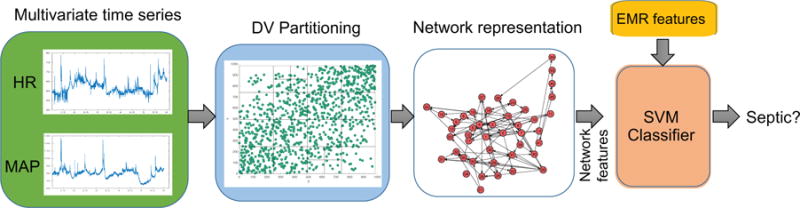
Schematic diagram of the proposed algorithm. The DV partitions obtained from the space of time-lagged HR and MAP time series are transformed to a network g - which consists of a set of nodes and an Adjacency matrix. Every time scale will have a corresponding network. Various topological attributes and features derived from the constructed networks are used as inputs to the SVM classifier. In addition to the network attributes, EMR features are also fed into the SVM classifier

Figure 2.

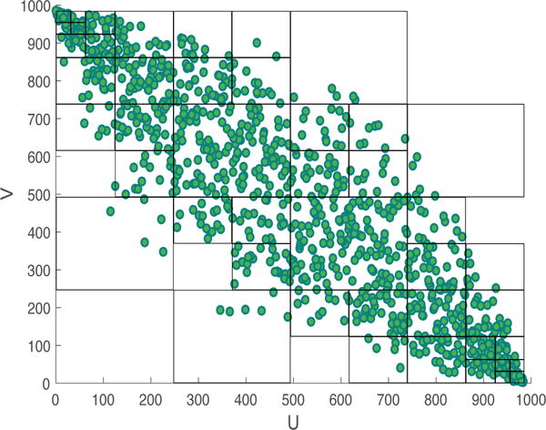
A two-dimensional visualization of DV partitioning. The observation space consists of 1,000 data points sampled from a bivariate Gaussian distribution with σ_xy = −0.9, ${\sigma }_x^2=1$, and ${\sigma }_y^2=1$. The figure shows the observation space after ordinal sampling. It can be observed that densely populated regions in the space have smaller partitions, in comparison to fewer partitions created in sparser areas.

The DV partitioning algorithm involves recursively dividing the state-space into more refined partitions, based on chi-squared test statistic that checks whether the data in the proposed partitioned cells are uniformly distributed. Let us consider a bivariate (2-dimensional) time series, X = [x₁, x₂, …, x_T] and Y = [y₁, y₂, …, y_T] where T is the length of the time series. First, a non-linear transformation is applied to X and Y, wherein the data in each time series are replaced by their rank orders (also called rank-order transformation). Let the rank order transformed time series be denoted by U and V respectively. We perform partitioning in the UV space as follows:

1. At every iteration, a bin (parent cell) is partitioned into smaller blocks (child cells) and we use the chi-squared test of independence to decide on the need for partitioning to child cells or not. The null hypothesis for the chi-squared test is that the sample distribution in the parent cell is uniform.

2. The chi-squared test statistic $\mathcal{S}$ is given by

   $$\mathcal{S}=\left({\displaystyle \sum _{i=1}^M{\left(\frac{{\displaystyle \sum N_i}}{M}-N_i\right)}^2}\right)/{\displaystyle \sum _{i=1}^M\left(\frac{N_i}{M}\right)}$$ (1)

   where, M is the total number of child cells for a parent cell, and N_i (i = 1, ….N) are the sample numbers.

3. For a 5% significance level with 3 degrees of freedom, if $\mathcal{S}$ is greater than ${\chi }_{95\%}^2$(3), then the distribution of data is not uniform and partitioning is continued. If not, the partitioning is stopped at that level. The level of statistical significance is a parameter that can be tuned.

4. At first, the observation space is partitioned at the medians of U, V margins to generate 4 child cells. And the Chi-square test of independence is performed, if partitioning condition holds, the child cells are split into further smaller blocks (partitioned at the medians of their respective margins), and this continues recursively until the Chi-square test statistic is no more satisfied across all cells.

The output of the partitioning algorithm is thus a list of partitions P, with each partition defined by a lower and upper bound in the observation space. An illustration of the DV partitioning algorithm for bivariate data is shown in figure 2 with the scatter plot of the data and the corresponding partitions obtained. It should be noted that the aforementioned procedure can be easily extended to any arbitrary N dimensional observation space.

2.2.3. Construction of network from partitions

Here we describe the process of construction of a network from a multivariate time series X. An example of a multivariate time series would be the HR and MAP time series recorded from a single subject. Given a list of partitions P, a map M: T ⇒ G can be defined from the time domain T to the network domain G. More formally, let us define a map M from time domain X ∈ T to a network g ∈ G, where X = {X₁, X₂, …, X_k}, k is the total number of time series recorded for each subject (in the above example, since HR and MAP are recorded for every subject, k = 2), and X_i ∈ ℝ^L, with L being the length of the time series, and g = {S, A} consisting of a set of nodes S and adjacency matrix A. The total number of nodes N correspond to the total number of partitions obtained from the DV partitioning algorithm. Therefore each partition p_i (i = 1, …N) is assigned to a node n_i ∈ N in the graph g. Every multidimensional data point in X is assigned to one of the partitions. The adjacency matrix A is a N×N matrix where a_ij corresponds to the transition from node n_i to node n_j. Two nodes n_i and n_j are connected in the network with a weight a_ij, with a_ij representing the total number of transitions from node n_i to n_j. Each partition p_i can be thought of as a dynamical state in a physiological system and the a_ij of the adjacency matrix represent the probability of transition between the dynamical states of the system. In the above example, we would thus construct one network from the bivariate time series (HR and MAP time series) recorded from the subject.

2.2.4. Multiscale Network representation

Interactions in biological systems manifest on multiple time scales (Bartsch et al. 2014), and the interactions may change in different ways at these different time scales. It may therefore be important to capture this multiscale nature of the interactions to help differentiate between healthy and unhealthy individuals. For a one dimensional time series [x₁, x₂, …, x_N], a coarse grained time series {y^(τ)}, corresponding to the scale factor τ was constructed as follows: First, the original times series was divided into non-overlapping windows of length τ; second, the data points inside each window were averaged. In our experiments, we coarse grained both HR and MAP according to the scale factor τ. Thus, for every scale factor τ_i (i = 1, …M), where M is the total number of scale factors, a network G_i (i = 1, …M) was constructed. Figure 3 provides a visualization of the networks constructed from bivariate time series (HR and MAP) of a control and a pre-septic patient at different time scales.

Figure 3.

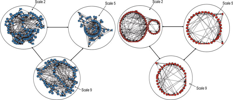
Examples of networks constructed from bivariate time series (HR and MAP) of a control (left panel) and a pre-septic (right panel) patient at different time scales. Within each of the networks, the arrows represent the transition from one node to another.

2.2.5. Network attributes for classification

In our proposed algorithm, for the network that we obtain as described in the previous sections, we compute many topological attributes and use the derived features for classification. The following network attributes were computed for every network in the dataset: number of nodes (total number of nodes in the network), number of edges (total number of edges in the network), Link density (defined as the total number of edges divided by the maximum possible edges in the network), average degree (the average value of the degree of all nodes in the network, where the degree of a node is defined as the total number of its neighboring edges), number of loops (the total number of independent loops in the network, also know as the “cyclomatic number” or the number of edges that need to be removed so that the network cannot have cycles), Loop3 (the total number of loops of size 3 in the network), Loop4 (the total number of loops of size 4 in the network), average clustering coefficient (the clustering coefficient c(u) for node u can be defined as the ratio of the number of actual edges between the neighbors of u to the number of possible edges between them, and the average clustering coefficient C(G) of a network is the average of c(u) taken over all the nodes in the network), Pearson coefficient (the pearson correlation coefficient for a degree sequence, also known as the assortativity coefficient (Newman 2002)), Algebraic connectivity (the second smallest Eigen value of the Laplacian matrix of a network, where the Laplacian matrix of a network is the difference between the sum of degrees of the diagonal elements in adjacency matrix and the adjacency matrix), Closeness (the closeness centrality, cc(u) for node u is the inverse of sum of distance from node u to all other nodes in the network, where the closeness centrality of a graph is the average mean of the above is the average of cc(u) taken over all the nodes in the network, Average eccentricity (eccentricity of a node u is defined as e(u) = max {d(u, v): v ∈ V}, where the distance d(u, v) is the length of the shortest path from u to v, and V is the set of all nodes. The average effective eccentricity is the average of effective eccentricities over all nodes in the network), Maximum effective eccentricity (Also known as the effective diameter, is defined as the maximum value of effective eccentricity over all nodes in the graph), Spectral radius (defined as the largest magnitude eigenvalue of the adjacency matrix of the network), Trace (sum of the eigenvalues of the adjacency matrix, i.e., Σλ, and Energy (squared sum of the eigenvalues of the adjacency matrix A. More formally, the energy of a network G is: $E(G)={\displaystyle {\sum }_i^n{\lambda }_i^2}$).

2.2.6. Entropy and other EMR features

For every subject, their socio-demographics features (Age, Gender, Weight, Race) were collected. We also included features that were commonly recorded by the bedside nurses including, Mean Arterial Pressure (MAP), Heart Rate (HR), Peripheral capillary Oxygen Saturation (SpO₂), Systolic Blood Pressure (SBP), Diastolic Blood Pressure (DBP), Respiration Rate (Resp), Glasgow Coma Score (GCS), and Temperature (Temp). Each of the above mentioned features were quantized into 8 levels, and each level was encoded into dummy binary representations. And these discretized representations were used in the classification model. We also extracted a few features that capture history, comorbidity, and the clinical context of the patient, including Charlson Comorbidity Index, Mechanical Ventilation, Unit Information (surgical, cardiac care, or neuro-intensive care), as well as Surgical Speciality (cardiovascular, neuro, ortho-spine, oncology, urology, etc) and Wound Type (clean, contaminated, dirty, or infected) if the patient had a surgery in past 12 hours.

We also calculated the following features from the HR and MAP time series (2 second resolution) derived from the bedside monitors proprietary software from the ECG and BP waveforms: standard Deviation of HR (HR_STD), Standard Deviation of MAP (MAP_STD), Multiscale Entropy (Costa et al. 2002) of (60/HR or RR intervals) and MAP (Over 17 Scales; RR_MSE, and MAP_MSE respectively)

2.3. Feature selection and classification

For every subject in the dataset, networks were constructed for time scales 1 through 10. A total of 16 network attributes were extracted from every constructed network. It is to be noted that the HR and MAP were each processed with a lag of order l. In addition to the network attributes, the Entropy and EMR features as described in Section 2.2.6 were extracted. All the features were then used to train a Support Vector Machine (SVM) classifier to predict onset of sepsis four hours ahead of time, based on the data from preceding six hours. The output of the SVM was the probability of membership in the Sepsis class. Hyper-parameters of the model including the time scale factors, and lag order l were optimized using Bayesian Optimization technique (Ghassemi et al. 2014).

For all continuous variables, we have reported the medians with Inter-Quartile range (IQR), and utilized a two-sided Wilcoxon ranksum test when comparing the septic and control populations. For binary features, we have reported the percentages, and utlized a two-sided Chi-square test to assess differences in proportions between the septic and control populations. To assess the performance of the proposed algorithm on out-of-sample data, we performed a 10 fold cross validation study. The features in training set were transformed to have Gaussian distributions using either the identity, square root or logarithmic transformations. The transformation which provided the lowest k-statistic using the Lilliefors test was used on both training and test sets. The transformed data (both training and test data) was then normalized by subtracting the mean computed from the training set and dividing by the standard deviation computed from the training set. Feature transformation, training, and classifier evaluation was performed separately for all the ten folds. Area Under the Receiver Operating Characteristic (AUROC) curve, accuracy, and specificity were calculated for training and test sets for all the folds. The sensitivity level was fixed at 0.85. We combined all the predictions (probability of being septic) across all the 10 folds to report a single pooled AUROC (Airola et al. 2009).

3. Results

A total of 250 subjects were considered for this study. The median [IQR] age for the septic and control subjects was 63 [47.5 72.5] and 59.5 [46.0 68.0] respectively. The patient characteristics of the entire dataset have been tabulated in table 1. It can be observed that the onset of sepsis is associated with a drop in MAP as well as SBP, DBP, and a significant increase in HR (92.5 vs. 84.8) and a significant decrease GCS (9.7 vs. 14.5), reflecting a moderate loss of consciousness or alertness.

Table 1.

Patient characteristics in the dataset

	Control	Septic	p-value
N	100	150	–
Age	59.5 [46.0 68.0]	63.0 [47.5 72.5]	0.15
Male(%)	56%	48%	0.21
MAP	81.7 [75.0 90.1]	78.5 [70.3 91.3]	0.22
HR	84.8 [73.2 97.6]	92.5 [75.1 110.0]	<0.01
SpO2	97.6 [96.3 99.3]	97.9 [95.1 99.5]	0.32
SBP	126.0 [111.7 143.7]	121.2 [103.3 143.3]	0.20
DBP	60.0 [55.0 66.7]	58.3 [52.5 67.2]	0.25
Respiration Rate	16.8 [14.2 18.7]	16.2 [2.25 20.4]	0.3
GCS	14.5 [10.0 15.0]	9.7 [6.0 14.3]	<0.01

3.1. Construction of network based on HR and MAP

The most commonly selected scales and embedding dimension by the Bayesian Optimization were scales 2, 3, 5, 6, 7, 9, and 10, lag order of 3. We therefore fixed these parameters across all experiments and model comparisons. We employed feature selection to find a minimum of set of relevant features. The most commonly selected features across all scales included the average clustering coefficient, pearson correlation coefficient, spectral radius, energy of graph, Trace, and number of loops of size 4.

In the following experiments we used the graph attributes alone as features for the classifier. First, we constructed multiscale networks from HR alone, and the pooled testing AUROC was 0.61. Next, we constructed multiscale networks from MAP alone, and the pooled testing AUROC was 0.61. By combining HR and MAP, and constructing multiscale networks achieved a pooled testing AUROC of 0.78.

3.2. Classifier trained on combination of Network, entropy and EMR features

Seven separate models were constructed, based on, 1) multiscale entropy (MSE) features calculated from the HR and MAP time series, 2) EMR features including patient demographics, and other features described in Section 2.2.6, 3) features extracted from Multiscale Network Representation (MSNR), 4) combining the EMR features and Entropy features (MSE + EMR), 5) combining MSNR and EMR features, 6) combining MSNR and MSE features, and 7) combining the EMR, MSNR and MSE features. The performance of each of the above models have been tabulated in table 2. The model based on MSNR features alone achieved a pooled testing AUROC of 0.78, with a corresponding sensitivity of 0.85 and specificity of 0.56. Combining the MSE features and MSNR features did not result in any improvement of AUROC (statistically insignificant). Combining EMR features and the MSNR features resulted in an improvement in AUC from 0.78 to 0.79 (statistically significant). For the model corresponding to MSNR + MSE + EMR features, the pooled AUROC on test set was 0.80 (statistically significant), with a specificity of 0.57 at 0.85 sensitivity level. The Receiver Operating Characteristic (ROC) curves for the above models have been plotted in figure 4.

Table 2.

Performance summary of classifier trained on combinations of network, entropy and EMR features. Values shown are pooled AUROCs

Model	Training AUROC	Testing AUROC
MSE	0.72	0.66
EMR	0.79	0.70
MSNR (MAP + HR)	0.85	0.78
MSE + EMR	0.83	0.73
MSNR + EMR	0.89	0.79
MSNR + MSE	0.85	0.75
MSNR + MSE + EMR	0.89	0.80

Figure 4.

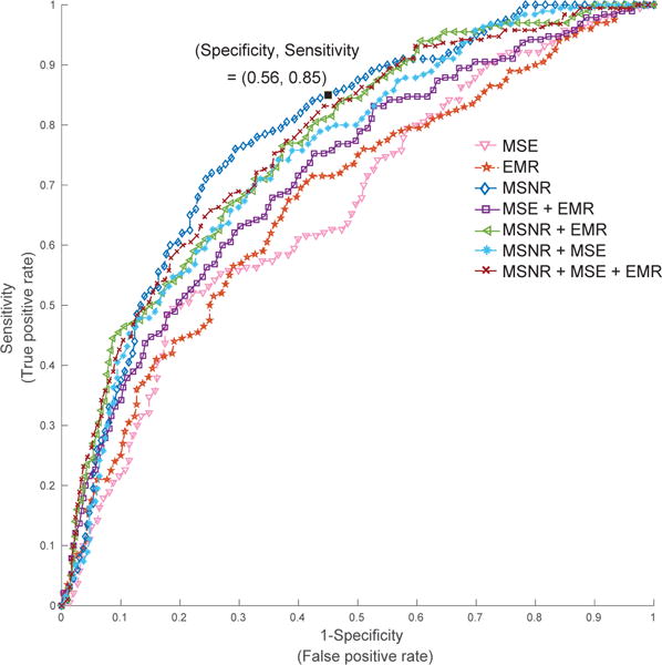
ROC curves for models based on combinations of network, entropy and EMR features. For the model corresponding to MSNR + MSE + EMR features, the AUROC on test set was 0.80, with a specificity of 0.57 at 0.85 sensitivity level. Notably, MSNR features alone achieved an AUC of 0.78, with the corresponding sensitivity (0.85) and specificity (0.56) marker on the plot

4. Discussion

We have shown that features derived from a multiscale HR and MAP time series network provide approximately 20% improvement in the area under the receiver operating characteristic (AUROC) for four hours ahead prediction of sepsis over traditional indices of heart rate entropy. This improvement is attributable to the information embedded in the higher order interaction of HR and MAP time series, as well as the proposed novel approach to network construction that utilizes adaptive partitioning of the state-space to define a set of discrete states. This discretization method naturally trades off uncertainty in defining an event (a unique state) for a more accurate estimation of the probability of the event. The resulting algorithm is quick to implement and readily extensible to multiscale analysis of the time series networks. Our final model, which includes the most commonly available clinical measurements in patients electronic medical record (EMR), multiscale entropy features as well as the proposed network-based features, achieved an AUROC of 0.80 on the testing set.

The proposed network construction technique takes advantage of the fact that the mutual information between a set of random variables is invariant to invertible transformations such as the rank order transformation (replacing the data by their ranks). The rank order transformation makes the proposed technique robust to time series outliers samples with high amplitudes. Moreover, time-lagged embedding provides information on the underlying dynamical system without having direct access to all the system variables (Takens et al. 1981). By applying the DV partitioning algorithm on the space of time-lagged embedded HR and MAP time series we arrive at states that capture the nonlinear dynamics of HR and MAP. Similar to the method of variable-bandwidth kernel density estimation (Terrell et al. 1992), the DV partitioning algorithm automatically adjusts the bin size (hypercubes), depending on the density and local distribution of the data points, but requires no a priori assumption on the Kernel bandwidth and is computationally more efficient to evaluate (Lee et al. 2012).

Some of the most important features including the average clustering coefficient are reflective of modularity of the network; networks with high modularity have dense connections between the nodes within modules but sparse connections between nodes in different modules. In graph theory, a clustering coefficient is a measure of the degree to which nodes in a graph tend to cluster together. Further study is needed to assess the correlation between the network features considered in this work and other commonly used predictive features within the literature. However, we hypothesize that the proposed framework provides a more generalizable set of features that are highly descriptive of the break down in autoregulatory mechanisms, and predictive of the eventual physiological decompensations, as in the case of sepsis. Notably, the multiscale nature of the proposed features provides robustness to the varying durations and time-scales of physiological deterioration in critically care patients.

Many methods have been proposed in the literature to study human physiology as a complex network of interactions among body organs and processes. Much of the effort have been concentrated on identification and quantification of the interactions between these physiological processes (Ivanov et al. 2014). Bashan et al. (Bashan et al. 2012) proposed the concept of time delay stability (TDS) to quantify the dynamic interactions among physiological processes, such as sleep and cardio-respiratory coupling. Building upon the concept of TDS, interactions across time scales and frequency bands have been explored to reveal dynamic interactions across body organs (Bartsch et al. 2015, Liu et al. 2015, Lin et al. 2016). Utilizing the concept of “information dynamics”, entropy-based approaches have been proposed to quantify the information transfer between physiological processes (Faes et al. 2014, Lee et al. 2012). Our proposed MSNR approach complements other pioneering works in “Network Physiology“ by introducing a non-parametric approach to partitioning the state-space, and taking advantage of network analysis to quantify the non-linear interactions among multiple physiological time series.

Clinical decision support tools can help identify those at the highest risk for future sepsis. Although, the existing works on utilizing EMR and laboratory data for prediction of sepsis seem promising (Lukaszewski et al. 2008; Wang et al. 2010; Desautels et al. 2016), they are limited by low-frequency, and often inconsistent data collected for purposes other than timely and accurate representation of patients’ physiology. Highly predictive features extracted directly extracted from the high-resolution vital signs time series can improve sepsis prediction over low-resolution clinical data in the ICU patients, and a high-performance prediction model can be derived from a combination of EMR and high-frequency physiologic data. A real-time system capable of early prediction of sepsis, followed by appropriate antibiotics therapy, will have a significant impact on the overall mortality and cost burden of this deadly disease (Seymour et al. 2017).

References

- Airola A, Pahikkala T, Waegeman W, et al. A comparison of AUC estimators in small-sample studies. Machine Learning in Systems Biology. 2009:3–13. [Google Scholar]
- Bartsch RP, Liu KK, Bashan A, et al. Network physiology: how organ systems dynamically interact. PLOS ONE. 2015;10(11):e0142143. doi: 10.1371/journal.pone.0142143. [DOI] [PMC free article] [PubMed] [Google Scholar]
- Bartsch RP, Liu KK, Ma QD, et al. Computing in Cardiology Conference (CinC), 2014. IEEE; 2014. Three independent forms of cardio-respiratory coupling: transitions across sleep stages; pp. 781–784. [PMC free article] [PubMed] [Google Scholar]
- Bashan A, Bartsch RP, Kantelhardt JW, et al. Network physiology reveals relations between network topology and physiological function. Nature Communications. 2012;3:702. doi: 10.1038/ncomms1705. [DOI] [PMC free article] [PubMed] [Google Scholar]
- Buchman TG. Physiologic stability and physiologic state. Journal of Trauma and Acute Care Surgery. 1996;41(4):599–605. doi: 10.1097/00005373-199610000-00002. [DOI] [PubMed] [Google Scholar]
- Buchman TG. Nonlinear dynamics, complex systems, and the pathobiology of critical illness. Current Opinion in Critical Care. 2004;10(5):378–382. doi: 10.1097/01.ccx.0000139369.65817.b6. [DOI] [PubMed] [Google Scholar]
- Campanharo AS, Sirer MI, Malmgren RD, et al. Duality between time series and networks. PLOS ONE. 2011;6(8):e23378. doi: 10.1371/journal.pone.0023378. [DOI] [PMC free article] [PubMed] [Google Scholar]
- Costa M, Goldberger AL, Peng CK. Multiscale entropy analysis of complex physiologic time series. Physical Review Letters. 2002;89(6):068102. doi: 10.1103/PhysRevLett.89.068102. [DOI] [PubMed] [Google Scholar]
- Desautels T, Calvert J, Hoffman J, et al. Prediction of sepsis in the intensive care unit with minimal electronic health record data: a machine learning approach. Journal of Medical Internet Research Medical Informatics. 2016;4:3. doi: 10.2196/medinform.5909. [DOI] [PMC free article] [PubMed] [Google Scholar]
- Duch J, Arenas A. Community detection in complex networks using extremal optimization. Physical Review E. 2005;72(2):027104. doi: 10.1103/PhysRevE.72.027104. [DOI] [PubMed] [Google Scholar]
- Faes L, Nollo G, Jurysta F, et al. Information dynamics of brain–heart physiological networks during sleep. New Journal of Physics. 2014;16(10):105005. [Google Scholar]
- Fortunato S. Community detection in graphs. Physics Reports. 2010;486(3):75–174. [Google Scholar]
- Ghassemi M, Lehman L-W, Snoek J, et al. Computing in Cardiology Conference (CinC), 2014. IEEE; 2014. Global optimization approaches for parameter tuning in biomedical signal processing: A focus on multi-scale entropy; pp. 993–996. [Google Scholar]
- Ghosh S, Li J, Cao L, et al. Septic shock prediction for ICU patients via coupled HMM walking on sequential contrast patterns. Journal of Biomedical Informatics. 2017;66:19–31. doi: 10.1016/j.jbi.2016.12.010. [DOI] [PubMed] [Google Scholar]
- Girvan M, Newman ME. Community structure in social and biological networks. Proceedings of the National Academy of Sciences. 2002;99(12):7821–7826. doi: 10.1073/pnas.122653799. [DOI] [PMC free article] [PubMed] [Google Scholar]
- Goldberger AL. Heartbeats, hormones, and health: is variability the spice of life? American Journal of Respiratory and Critical Care Medicine. 2001;163(6):1289–1290. doi: 10.1164/ajrccm.163.6.ed1801a. [DOI] [PubMed] [Google Scholar]
- Henry KE, Hager DN, Pronovost PJ, et al. A targeted real-time early warning score (TREWScore) for septic shock. Science Translational Medicine. 2015;7(299):299ra122–299ra122. doi: 10.1126/scitranslmed.aab3719. [DOI] [PubMed] [Google Scholar]
- Hudson JE. Signal processing using mutual information. IEEE Signal Processing Magazine. 2006;23(6):50–54. [Google Scholar]
- Hug CW, Clifford GD, Reisner AT. Clinician blood pressure documentation of stable intensive care patients: an intelligent archiving agent has a higher association with future hypotension. Critical Care Medicine. 2011;39(5):1006. doi: 10.1097/CCM.0b013e31820eab8e. [DOI] [PMC free article] [PubMed] [Google Scholar]
- Huston JM, Tracey KJ. The pulse of inflammation: heart rate variability, the cholinergic anti-inflammatory pathway and implications for therapy. Journal of Internal Medicine. 2011;269(1):45–53. doi: 10.1111/j.1365-2796.2010.02321.x. [DOI] [PMC free article] [PubMed] [Google Scholar]
- Ivanov PC, Amaral LAN, Goldberger AL, et al. Multifractality in human heartbeat dynamics. Nature. 1999;399(6735):461–465. doi: 10.1038/20924. [DOI] [PubMed] [Google Scholar]
- Ivanov PC, Bartsch RP. Networks of Networks: the last Frontier of Complexity. Springer; 2014. Network physiology: mapping interactions between networks of physiologic networks; pp. 203–222. [Google Scholar]
- Lacasa L, Nicosia V, Latora V. Network structure of multivariate time series. Scientific Reports. 2015;5 doi: 10.1038/srep15508. [DOI] [PMC free article] [PubMed] [Google Scholar]
- Lee J, Nemati S, Silva I, et al. Transfer entropy estimation and directional coupling change detection in biomedical time series. Biomedical Engineering Online. 2012;11(1):19. doi: 10.1186/1475-925X-11-19. [DOI] [PMC free article] [PubMed] [Google Scholar]
- Lehman L-WH, Adams RP, Mayaud L, et al. A physiological time series dynamics-based approach to patient monitoring and outcome prediction. IEEE Journal of Biomedical and Health Informatics. 2015;19(3):1068–1076. doi: 10.1109/JBHI.2014.2330827. [DOI] [PMC free article] [PubMed] [Google Scholar]
- Lin A, Liu KK, Bartsch RP, et al. Delay-correlation landscape reveals characteristic time delays of brain rhythms and heart interactions. Philosophical Transactions of the Royal Society A. 2016;374(2067):20150182. doi: 10.1098/rsta.2015.0182. [DOI] [PMC free article] [PubMed] [Google Scholar]
- Liu KK, Bartsch RP, Lin A, et al. Plasticity of brain wave network interactions and evolution across physiologic states. Frontiers in Neural Circuits. 2015;9 doi: 10.3389/fncir.2015.00062. [DOI] [PMC free article] [PubMed] [Google Scholar]
- Lukaszewski RA, Yates AM, Jackson MC, et al. Presymptomatic prediction of sepsis in intensive care unit patients. Clinical and Vaccine Immunology. 2008;15(7):1089–1094. doi: 10.1128/CVI.00486-07. [DOI] [PMC free article] [PubMed] [Google Scholar]
- Luque B, Lacasa L, Ballesteros F, et al. Horizontal visibility graphs: Exact results for random time series. Physical Review E. 2009;80(4):046103. doi: 10.1103/PhysRevE.80.046103. [DOI] [PubMed] [Google Scholar]
- Mancia G. Short-and Long-term blood pressure variability. Hypertension. 2012;60(2):512–517. doi: 10.1161/HYPERTENSIONAHA.112.194340. [DOI] [PubMed] [Google Scholar]
- MATLAB. version 9.1 (R2016b) Natick, Massachusetts: The MathWorks Inc; 2016. [Google Scholar]
- Moorman JR, Delos JB, Flower AA, et al. Cardiovascular oscillations at the bedside: early diagnosis of neonatal sepsis using heart rate characteristics monitoring. Physiological Measurement. 2011;32(11):1821. doi: 10.1088/0967-3334/32/11/S08. [DOI] [PMC free article] [PubMed] [Google Scholar]
- Nemati S, Edwards BA, Lee J, et al. Respiration and heart rate complexity: effects of age and gender assessed by band-limited transfer entropy. Respiratory Physiology & Neurobiology. 2013;189(1):27–33. doi: 10.1016/j.resp.2013.06.016. [DOI] [PMC free article] [PubMed] [Google Scholar]
- Newman ME. Assortative mixing in networks. Physical Review Letters. 2002;89(20):208701. doi: 10.1103/PhysRevLett.89.208701. [DOI] [PubMed] [Google Scholar]
- Nicolis G, Cantu AG, Nicolis C. Dynamical aspects of interaction networks. International Journal of Bifurcation and Chaos. 2005;15(11):3467–3480. [Google Scholar]
- Parati G, Ochoa JE, Lombardi C, et al. Blood pressure variability: assessment, predictive value, and potential as a therapeutic target. Current Hypertension Reports. 2015;17(4):23. doi: 10.1007/s11906-015-0537-1. [DOI] [PubMed] [Google Scholar]
- Quinn JA, Williams CK, McIntosh N. Factorial switching linear dynamical systems applied to physiological condition monitoring. IEEE Transactions on Pattern Analysis and Machine Intelligence. 2009;31(9):1537–1551. doi: 10.1109/TPAMI.2008.191. [DOI] [PubMed] [Google Scholar]
- Seymour CW, Gesten F, Prescott HC, et al. Time to treatment and mortality during mandated emergency care for sepsis. New England Journal of Medicine. 2017 doi: 10.1056/NEJMoa1703058. [DOI] [PMC free article] [PubMed] [Google Scholar]
- Seymour CW, Liu VX, Iwashyna TJ, et al. Assessment of clinical criteria for sepsis: for the Third International Consensus Definitions for Sepsis and Septic Shock (Sepsis-3) The Journal of the American Medical Association. 2016;315(8):762–774. doi: 10.1001/jama.2016.0288. [DOI] [PMC free article] [PubMed] [Google Scholar]
- Steinhauser D, Krall L, Müssig C, et al. Correlation networks. Analysis of Biological Networks. 2008:305–333. [Google Scholar]
- Sun J, Deem MW. Spontaneous emergence of modularity in a model of evolving individuals. Physical Review Letters. 2007;99(22):228107. doi: 10.1103/PhysRevLett.99.228107. [DOI] [PubMed] [Google Scholar]
- Takens F, et al. Detecting strange attractors in turbulence. Lecture notes in Mathematics. 1981;898(1):366–381. [Google Scholar]
- Terrell GR, Scott DW. Variable kernel density estimation. The Annals of Statistics. 1992:1236–1265. [Google Scholar]
- Wang SL, Wu F, Wang BH. Advances in Computational Biology. Springer; 2010. Prediction of severe sepsis using SVM model; pp. 75–81. [DOI] [PubMed] [Google Scholar]
- Yang Y, Yang H. Complex network-based time series analysis. Physica A: Statistical Mechanics and its Applications. 2008;387(5):1381–1386. [Google Scholar]