Network embedding-based representation learning for single cell RNA-seq data

Abstract

Single cell RNA-seq (scRNA-seq) techniques can reveal valuable insights of cell-to-cell heterogeneities. Projection of high-dimensional data into a low-dimensional subspace is a powerful strategy in general for mining such big data. However, scRNA-seq suffers from higher noise and lower coverage than traditional bulk RNA-seq, hence bringing in new computational difficulties. One major challenge is how to deal with the frequent drop-out events. The events, usually caused by the stochastic burst effect in gene transcription and the technical failure of RNA transcript capture, often render traditional dimension reduction methods work inefficiently. To overcome this problem, we have developed a novel Single Cell Representation Learning (SCRL) method based on network embedding. This method can efficiently implement data-driven non-linear projection and incorporate prior biological knowledge (such as pathway information) to learn more meaningful low-dimensional representations for both cells and genes. Benchmark results show that SCRL outperforms other dimensional reduction methods on several recent scRNA-seq datasets.

INTRODUCTION

High-throughput RNA sequencing is widely used for studying transcriptomes. Since the traditional bulk RNA-seq can only detect the average gene expression of a cell population, this technique is unable to quantify cell-to-cell heterogeneity. With the advent of new single-cell high-throughput RNA sequencing (scRNA-seq) technology (1–3), valuable insights into cell heterogeneity and transcriptional stochasticity can now be obtained.

Along with the technological breakthrough of scRNA-seq, it also raises new computational and analytical challenges. Due to the small amount of RNA transcripts in each cell, low capture efficiency and stochastically transcriptional bursts, scRNA-seq data contains excessive amount of drop out events (resulting in zero or near-zero transcript counts), which can complicate data analysis and biological discovery. Until now, many existing methods (4–6) originally developed for bulk RNA-seq data are still being widely used in single cell studies. However, these methods cannot account for the unique features of scRNA-seq data. Dimension reduction of high-dimensional gene expression data is an essential step for visualization and downstream analysis. Nowadays, principal component analysis (PCA) (7) and t-distributed stochastic neighbor embedding (t-SNE) (8) are the two most widely used methods in gene expression data analysis. PCA, an eigen-decomposition analysis of data covariance matrix, finds a linear transformation of the originally high-dimensional data that maximizes the variance of the projected data. The assumption about the data is that it is normally distributed. t-SNE finds a non-linear low-dimensional space that preserves the similarities of the high-dimensional data. It models the similarity among data points by a probability distance based on Gaussian kernel rather than a Euclidean distance. So the assumption of t-SNE is that the local proximity can be measured by the Student’s t-distribution in the low-dimensional space. Both of them do not account for the effects of drop-out events which occur frequently in scRNA-seq data. A recently proposed method ZIFA (9) explicitly models drop-out events, which uses zero-inflated factor analysis to do dimension reduction. This method shows advantages over the traditional dimensional reduction methods for analyzing scRNA-seq data. However, the assumption behind ZIFA is that a drop-out event results in zero count, so it models exact zero rather than near-zero found in real scRNA-seq data. In addition, ZIFA assumes that the projection between the reduced subspace and the original data space is linear. The assumption about the data is that it is zero inflated Gaussian distributed. All of these three widely used methods have specific assumptions about the data. However, these assumptions imposed on the real data may result in a loss of power and accuracy.

In order to better learn the meaningful features from scRNA-seq data, we developed a data-driven and non-linear dimension reduction method named Single Cell Representation Learning (SCRL) based on network-based embedding technique (10). SCRL learns more meaningful representations for scRNA-seq data by considering the prior gene–gene association (such associations can be, for instance, derived from annotated pathways, protein–protein interaction networks or gene co-expression networks constructed from some related bulk RNA-seq data, etc.). In this way, even if the expression of a gene is dropped out as zero or near-zero, the low-dimensional representations can still provide some signals from its associated or covariant genes. We conducted experiments on several scRNA-seq datasets to demonstrate that SCRL can significantly outperform those existing methods. SCRL provides two unique advantages: (i) it can integrate both scRNA-seq data and prior biological knowledge for more insightful low-dimensional representations; and (ii) it can simultaneously learn a shared low-dimensional representation for both cells and genes. Consequently, the associations of cell clusters and genes can be explored by examining their correlations in the shared subspace.

MATERIALS AND METHODS

Overview

The basic idea of SCRL is to learn low-dimensional representations by preserving the cell-to-cell proximity and by integrating with the prior gene–gene network. The cells with similar gene expression patterns (constraint by the prior gene–gene network) should be projected to neighbor regions in the reduced subspace. As shown in Figure 1, the method SCRL consists of two steps, the first step is network construction: we construct a Cell-ContextGene network based on the scRNA-seq data and a Gene-ContextGene network based on pathway annotations. The context-genes are introduced in both networks for considering the shared information from the gene expression data and the pathway priors. This formulation is adapted from the concept of ‘context’ in natural language processing (10). In the second step, we combine these two networks and implement joint bipartite network embedding to learn low-dimensional representations for both the cells and the genes.

Figure 1.

Overview of SCRL. (A) Input data. The left matrix is the scRNA-seq data and the right matrix is the pathway data. (B) Network construction. SCRL builds a Cell-ContextGene network (left) based on the scRNA-seq data and a Gene-ContextGene network (right) based on the pathway annotations. In these two bipartite networks, the cells are colored blue, the context-genes are colored green and the genes are colored red. The context-genes are shared in the two networks. Then, SCRL combines these two bipartite networks to learn the low-dimensional vector representations for cells, genes and context-genes. (C) The low-dimensional representation matrixes for cells (blue), context-genes (green) and genes (red). Each row in the matrix represents a low-dimensional vector representation. (D) Visualization of the low-dimensional representations of the cells learned from SCRL.

Model

Network construction

Cell-ContextGene network

Given a scRNA-seq dataset with C cells and A context-genes, a bipartite Cell-ContextGene network E_ca was constructed as follows: an edge was added between the i-th cell and the j-th context-gene, if the corresponding expression y_ij > 0 (the weight of the edge is equal to y_ij).

Gene-ContextGene network

We constructed a bipartite Gene-ContextGene network E_ga based on the prior gene–gene interaction or the correlation knowledge (IntPath (11) in this study): an edge with weight 1 was added between the j*-th gene and the j-th context-gene, if the two genes directly connected according to the prior knowledge.

Joint bipartite network embedding

Joint bipartite network embedding aims to learn a mapping function from the original network space to a low-dimensional vector space through embedding multiple bipartite networks (Cell-ContextGene network and Gene-ContextGene network in this study).

Let C be the number of cells, A be the number of context-genes, G be the number of genes. c is a cell, a is a context-gene, g is a gene, we use i = 1,2,…,C to index over the cells, j = 1,2,…,A to index over the context-genes, to index over the genes. The low-dimensional representation of is , the low-dimensional representation of is , the low-dimensional representation of is , is the expression level of the context-gene j in the cell i, is the weight between the gene and the context-gene j. , where L is the dimension of the low-dimensional representations. For most applications, L varies from 100 to 500, for a balance of the computational time and the memory requirement.

We define the conditional probability that a context-gene in a cell as the following softmax function:

(1)

According to the observed data, its corresponding empirical distribution is:

(2)

(3)

In this way, we can get the conditional probability distribution of the cell over all the context-genes and the corresponding empirical conditional distribution .

For preserving the cell-to-cell similarity, naturally we would wish that the conditional distribution of the cell, which is specified by the low-dimensional representation, should be close to the empirical conditional distribution .

Therefore, our goal is to minimize the following objective function by using the Kullback–Leibler divergence(omitting some constants):

(4)

Similarly, we can also get the objective function of the Gene-ContextGene network:

(5)

In order to integrate these two sources of information, a straight forward way is to embed the two bipartite networks simultaneously. This can be achieved by minimizing the linear combination of and .The final objective function is therefore:

(6)

Finally, we can get the low-dimensional representations for both the cells and the genes. Here, is the weight for the Gene-ContextGene network. Experiments show that the performance is similar for a wide range of . So we set in the following analysis. However, directly optimizing the softmax term (Equation 1) is computationally expensive, as it needs summing over all context-genes, which could be very large. Hence, we adopted sampling-based strategies ‘Negative sampling’ (12) to overcome this problem. Negative sampling transforms the originally computation-expensive loss function into a binary classification proxy objective, which has the same parameters but with much lower computational complexity. The binary classification function aims to discriminate the genuine samples from the real data (the empirical distribution) versus the multiple random samples generated by the noise distribution. Specifically, the Equation (6) can be rewritten as the following objective function:

(7)

where, is the sigmoid function, K is the number of the negative samples (the default setting of K is 5). and are the noise (background control) distribution of the context-genes, which can be used to generate the negative samples.

We used asynchronous stochastic gradient descent algorithm to optimize the loss function (7). For a random sampled edge (i, j), the gradient will be multiplied by the weight of the edge. There would potentially be a serious problem if the weights of any edges had a large variance, which could have led to ‘gradient explosion and vanishing problem’. To overcome this, we used the edge sampling technique proposed previously by Tang (10). The basic idea is to split the weighted edge into several binary edges. For example, if the weight of edge (i, j) is 10, then we can transform this edge into 10 binary edges.

The algorithm can be summarized as follows:

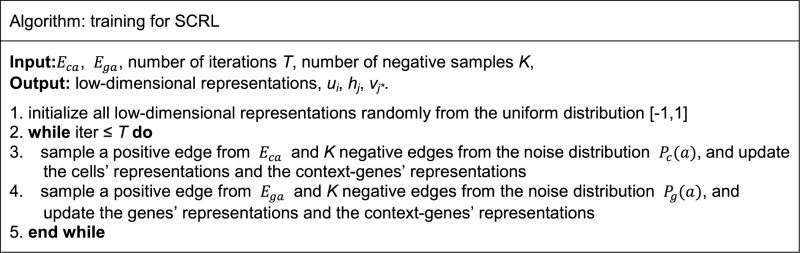
In practice, the iteration number T should be proportional to the maximum number of the edges of the two networks.

Performance comparison

We compared the performance of our method SCRL with PCA, t-SNE and ZIFA for cell type identification on three publicly available scRNA-seq datasets. Their cell types are known apriori, providing a golden standard. The datasets used in this study are listed in Table 1. Specifically, we compared our method SCRL with others from both aspects: ‘unsupervised’ (visualization and clustering) and ‘supervised’ (classification). Here, by default, we set the final dimension for the low-dimensional representation learnt by SCRL to be 200 (which may be adjusted by the user).

Table 1. A list of scRNA-seq datasets.

Dataset	Cells	Context genes	Genes
Guo (13)	330	14 807	5734
Petropoulos (14)	1529	19 651	5734
Pollen (15)	301	17 277	5734

In the unsupervised comparison, we firstly showed the cells in 2D, so that we can explore the data structure visually. For SCRL results, we used PCA to project the 200 dimensional representations to 2D for visualization. Then we used the WB-ratio metric (the ratio of average distance within/between clusters) to evaluate the cell separation, where represent different cells, represents the cells within the same cluster k, we use k = 1,2,…K to index over all clusters.

In the supervised comparison, we calculated the classification accuracy. For a fair comparison, we projected the data from the initial dimensions to 10 dimensions (the initial low-dimensional representations learnt by SCRL was 200 dimensions, so we used PCA to get the most important 10 principle components for the following analysis). Then we random sampled a certain proportion of the cells to train the classifiers using one-versus-the-rest linear SVM, and calculated the accuracy rate for the remaining test dataset. We repeated the process 20 times and got the final averaged accuracy rate.

At last, we found several significant pathways corresponding to each cell type on Guo's dataset. First, we filtered several cancer and drug-related pathways. Then we calculated the Spearman correlations between one cell type and the genes in each pathway in the low-dimensional representations. We can get some significant pathways among the top 10 percentage ranked pathways for each cell type according to the absolute value of Spearman correlation.

Datasets

We applied our method to three publicly available datasets (Table 1). Guo dataset (13) was from 330 single cells including primordial germ cells (PGC cells), somatic cells (SOMA cells) and inner cell mass cells (ICM cells). Petropoulos dataset (14) was from 1529 single cells representing continuous different embryonic stages (E3–E7) of 88 human preimplantation embryos. Pollen dataset (15) was from 301 single cells that including pluripotent cells, blood cells, skin cells and neural cells from 11 cell lines.

RESULTS

How to characterize the cell heterogeneity is a key question in single cell data analysis. So we compared our method SCRL with PCA, t-SNE and ZIFA for the cell type identification from the following two aspects: clustering/visualization and classification.

Clustering and visualization

We visualized the results of these datasets in 2D so that the structure of the data can be intuitively explored. Results in Figure 2A show that SCRL can separate the three clusters clearly on the Guo dataset. However, other dimension reduction methods mix the three clusters together. Especially for the rare ICM cells, only SCRL can distinguish them from other cell types. In addition, SCRL with gene–gene information shows better performance than SCRL without it. In the results of SCRL without prior information, ICM cells are still close to several SOMA cells. However, with the prior information, they are well separated. Results in Figure 2B show that for the Petropoulos dataset, SCRL can separate the cells more clearly than the other methods. In the results of SCRL, E6 and E7 cells are obviously separated comparing to other methods. Despite the five cell types are still somewhat mixed, it is expected as those cells used in the study representing a temporal progression, which is more apt to be a continuous time series than discrete cell types. In the low-dimensional space, we also showed the labels of cells which are picked several hours later than E4 cells (marked as E4.late) and several hours earlier than E5 cells (marked as E5.early) in the results, for a better understanding of the developmental process. We can observe that the cells are clearly ordered in agreement with the developmental time. In Figure 2C, for the four cell types in the Pollen dataset, all the methods have similarly good performances expect for ZIFA which behaves relatively worse.

Figure 2.

Performance comparison of the four-dimensional reduction methods for visualization on the three datasets. (A) Guo dataset. (B) Petropoulos dataset. (C) Pollen dataset. Each point represents a cell and the cell is colored according to its known cell type label. SCRL (no prior) represents the method without using the pathway information.

In order to measure the cell separation more quantitatively, we used the metric WB-ratio (ratio of average distance within/between clusters) to assess the cell separation in 2D, a smaller ratio means a better performance. As show in Figure 3, the quantitative results are indeed consistent with the intuitive visualization. The value of SCRL’s WB-ratio is the best comparing with the other three methods for these three datasets. Overall, these results indicate that SCRL has a superior unsupervised performance.

Figure 3.

Performance comparison of the four-dimensional reduction methods for within-cluster and between-cluster (WB) ratio on the three datasets. The x-axis represents different datasets and the y-axis represents WB-ratio (smaller ratio means better performance).

Classification

In general, the results in Figure 4 show that SCRL always has a better classification performance than PCA, t-SNE and ZIFA on these three datasets, when the proportion of training cells varies from 1 to 10%. The performance of SCRL is persistently better than others even as the proportion of training data decreases, which indicates that SCRL is more robust to the change in the number of training samples. More specifically, for the Guo dataset and the Petropoulos dataset, SCRL shows obvious improvements than PCA, t-SNE and ZIFA. For the Pollen dataset, these four methods have comparable performances, except that ZIFA had worse behavior for the lower proportion of training dataset. Regarding to the prior gene–gene information, the SCRL with the prior information consistently outperformed that without. All these results suggest that the prior biological network information can improve the cell classification performance. When the proportion of training cells varies from 5% to 95%, we can observe that t-SNE has poor performances even when 95% cells were used as training dataset. The other methods show comparable performances for the Guo and Pollen datasets when more than 50% cells were used for training(see Supplementary Figure S1). For the two datasets, we can see different cell populations can be easily separated based on the visualization results (Figure 2). However, for the Petropoulos dataset, the cells in some developmental stages are mixed. In that dataset, SCRL shows consistent better performances than the other methods. These results indicate that SCRL can better represent the heterogeneities when the differences between different cell populations are small.

Figure 4.

Performance comparison of the four-dimensional reduction methods for classification accuracy on the three datasets. (A) Guo dataset. (B) Petropoulos dataset. (C) Pollen dataset. The x-axis corresponds to the percentage (from 1 to 10%) of the cells for training classifier, each color represents one method. The y-axis represents the classification accuracy for the test data.

In addition, we tested the dimension sensitivity of SCRL on the three datasets. We set the percentage of training data as 10%. The dimension ranged from 10 to 1280. Given a fixed dimension of low-dimensional representations, we learned the low-dimensional representation for each cell. We randomly sampled 10% of cells to train the classifier by using the one-versus-the-rest linear SVM, and calculated the accuracy rate for the left 90% test cells. We repeated the process 20 times and got the final accuracy rate. The results of classification accuracy were shown in Figure 5A. Before the step of training the classifier, we used PCA to project the initial dimensional representations to 10D for classification, the results were shown in Figure 5B. We can observe that the classification accuracy of SCRL is not sensitive to the dimension number from 100 to 200 dimensions.

Figure 5.

Dimension sensitivity of SCRL on the three datasets. (A) Dimension sensitivity of SCRL. (B) Dimension sensitivity of SCRL after PCA. Each color corresponds to one dataset, the x-axis represents different dimensions, the y-axis represents the classification accuracy.

Finding the significant pathways for each cell type

SCRL gets the low-dimensional representations for both the genes and the cells simultaneously. By calculating the similarity between cell types and pathways based on the low-dimensional representations of the cells and the genes, we can extract the significant pathways corresponding to a specific cell type as a supplement to the GO enrichment. First, we calculated the mean representation of this cell type and the mean representation of each pathway. Then we calculated the Spearman correlation between them. Here we take the Guo dataset as an example, which aims at studying the development and regulation of human primordial germ cells (PGCs). They generated 11 ICM cells from the blastocysts, 233 PGCs (84 female PGCs and 149 male PGCs) and 86 SOMA cells. We extracted several interesting pathways among the top 10% ranked pathways for each cell type. As shown in Table 2, in ICM cells, we found the Wnt signaling pathway, the cell cycle pathway and the MAPK signaling pathway were among the top-ranked pathways. Among them, the Wnt signaling pathway is known to play an important role in regulating pluripotency (16). The cell cycle-related pathways are essential for the self-renewal and proliferation of ICM cells (17). The estrogen signaling pathway, the GnRH signaling pathway, the Wnt signaling pathway and the TGF Beta signaling pathway were ranked on top for the female PGCs, so were the GnRH signaling pathway and the Wnt signaling pathway for the male PGCs. Among them, the Wnt signaling pathway is essential in affecting PGC’s fate (18), and the TGF Beta signaling pathway is essential in modulating PGC mitosis (19). The GnRH signaling pathway and the gonadal hormones-related pathway are important in PGC cells (20). For SOMA cells, the B-cell receptor signaling pathway, the T-cell receptor signaling pathway and the Oocyte meiosis pathway were identified. For the Oocyte meiosis pathway, as reported in a recent study (21), SOMA cells could secrete Retinoic Acid, which is the key signal for induction of meiosis.

Table 2. Significant pathways corresponding to each cell type.

Cell type	Significant pathway	Rank
ICM cell	Wnt signaling pathway	9
	Cell cycle	12
	MAPK signaling pathway	13
Female PGC cell	Estrogen signaling	8
	GnRH signaling pathway	19
	Wnt signaling pathway	35
	TGF beta signaling pathway	37
Male PGC cell	GnRH signaling pathway	30
	Wnt signaling pathway	44
SOMA cell	B cell receptor signaling pathway	10
	T cell receptor signaling pathway	16
	Oocyte meiosis	19

In addition, we projected several marker genes and all cells in the same space. As shown in Supplementary Figures S2 and 3, interestingly, we could observe that the pluripotency marker genes POU5F1 and NANOG, the germline marker genes KIT, ALPL, SOX17 and CD38 were closely linked to the PGCs (The details are in the Supplementary File). As shown in Supplementary Table S1, the Euclidean distance between the selected marker gene and the cell type is consistent with the visualization. This result further supports the utility of the joint embedding for both the cells and the genes.

DISCUSSION

In summary, our results demonstrate that SCRL outperforms other existing dimensional reduction methods based on different criteria in the study of the cell heterogeneity. In addition, the edge-sampling based optimization method ensures the efficiency and the effectiveness, which is able to handle large datasets (the detailed runtime comparison is shown in Supplementary Figure S5). Furthermore, SCRL offers a novel integrative framework for the comprehensive single cell heterogeneity analysis. It can simultaneously integrate multiple sources of network information for learning low-dimensional representations, hence overcoming the high noise of scRNA-seq data. For a proof of principle, here we combined scRNA-seq data and pathway information. This framework may be extended to integrate scRNA-seq data with bulk RNA-seq data, mass cytometry data, etc., which is specially promising in future single cell multi-omics data analysis. In addition, SCRL can project cells and genes into a common (shared) subspace, therefore providing a novel way to further explore the relationship between genes and cells.

Bringing in prior pathway information can help reduce the effects of drop-out events to some extent. However, just as every coin has two sides, the gene pair information that IntPath has provided only includes a subset of the full reference genes, so the low representations learnt for the genes are incomplete. This incompleteness could reduce the power of SCRL for finding marker genes and significant pathways. After getting the low-dimensional representations for both the genes and the cells, we adopted a simple straightforward way to explore the relationship between them. Further experiments would be required to narrow down and validate any predicted marker genes and significant pathways.

DATA AVAILABILITY

A C++ based software implementation of SCRL is made freely available online via https://github.com/SuntreeLi/SCRL.

SUPPLEMENTARY DATA

Supplementary Data are available at NAR Online.

FUNDING

National Nature Science Foundation of China [31301044, 31671384, 31361163004, 61370035]; National Basic Research Program of China [2017YFA0505500]; Tsinghua National Laboratory for Information Science and Technology Cross-discipline Foundation; NIH [MH102616 to M.Q.Z.].

Conflict of interest statement. None declared.

REFERENCES

- 1. Tang F., Barbacioru C., Wang Y., Nordman E., Lee C., Xu N., Wang X., Bodeau J., Tuch B.B., Siddiqui A. et al. . mRNA-Seq whole-transcriptome analysis of a single cell. Nat. Methods. 2009; 6:377–382. [DOI] [PubMed] [Google Scholar]
- 2. Wu A.R., Neff N.F., Kalisky T., Dalerba P., Treutlein B., Rothenberg M.E., Mburu F.M., Mantalas G.L., Sim S. et al. . Quantitative assessment of single-cell RNA-sequencing methods. Nat. Methods. 2014; 11:41–46. [DOI] [PMC free article] [PubMed] [Google Scholar]
- 3. Kolodziejczyk A.A., Kim J.K., Svensson V., Marioni J.C., Teichmann S.A.. The technology and biology of single-cell RNA sequencing. Mol. Cell. 2015; 58:610–620. [DOI] [PubMed] [Google Scholar]
- 4. Anders S., Huber W.. Differential expression analysis for sequence count data. Genome Biol. 2010; 11:R106. [DOI] [PMC free article] [PubMed] [Google Scholar]
- 5. Trapnell C., Roberts A., Goff L., Pertea G., Kim D., Kelley D.R., Pimentel H., Salzberg S.L., Rinn J.L., Pachter L.. Differential gene and transcript expression analysis of RNA-seq experiments with TopHat and Cufflinks. Nat. Protoc. 2012; 7:562–578. [DOI] [PMC free article] [PubMed] [Google Scholar]
- 6. Robinson M.D., McCarthy D.J., Smyth G.K.. edgeR: a Bioconductor package for differential expression analysis of digital gene expression data. Bioinformatics. 2010; 26:139–140. [DOI] [PMC free article] [PubMed] [Google Scholar]
- 7. Wold S., Esbensen K., Geladi P.. Principal Component Analysis. Chemometrics and intelligent laboratory systems. 1987; 2:37–52. [Google Scholar]
- 8. Maaten L.V.D., Hinton G.. Visualizing data using t-SNE. J. Mach. Learn. Res. 2008; 9:2579–2605. [Google Scholar]
- 9. Pierson E., Yau C.. ZIFA: dimensionality reduction for zero-inflated single-cell gene expression analysis. Genome Biol. 2015; 16:241. [DOI] [PMC free article] [PubMed] [Google Scholar]
- 10. Tang J., Qu M., Wang M., Zhang M., Yan J., Mei Q.. Line: large-scale information network embedding. Proceedings of the 24th International Conference on World Wide Web. 2015; Florence: 1067–1077. [Google Scholar]
- 11. Zhou H., Jin J., Zhang H., Yi B., Wozniak M., Wong L.. IntPath–an integrated pathway gene relationship database for model organisms and important pathogens. BMC Syst. Biol. 2012; 6:S2. [DOI] [PMC free article] [PubMed] [Google Scholar]
- 12. Mikolov T., Sutskever I., Chen K., Corrado G.S., Dean J.. Burges CJC, Bottou L, Welling M, Ghahramani Z, Weinberger KQ. Distributed representations of words and phrases and their compositionality. Advances in Neural Information Processing Systems. 2013; Lake Tahoe: 3111–3119. [Google Scholar]
- 13. Guo F., Yan L., Guo H., Li L., Hu B., Zhao Y., Yong J., Hu Y., Wang X., Wei Y. et al. . The transcriptome and DNA methylome landscapes of human primordial germ cells. Cell. 2015; 161:1437–1452. [DOI] [PubMed] [Google Scholar]
- 14. Petropoulos S., Edsgärd D., Reinius B., Deng Q., Panula S.P., Codeluppi S., Plaza Reyes A., Linnarsson S., Sandberg R., Lanner F.. Single-cell RNA-seq reveals lineage and X chromosome dynamics in human preimplantation embryos. Cell. 2016; 165:1012–1026. [DOI] [PMC free article] [PubMed] [Google Scholar]
- 15. Pollen A.A., Nowakowski T.J., Shuga J., Wang X., Leyrat A.A., Lui J.H., Li N., Szpankowski L., Fowler B., Chen P. et al. . Low-coverage single-cell mRNA sequencing reveals cellular heterogeneity and activated signaling pathways in developing cerebral cortex. Nat. Biotechnol. 2014; 32:1053–1058. [DOI] [PMC free article] [PubMed] [Google Scholar]
- 16. Sokol S.Y. Maintaining embryonic stem cell pluripotency with Wnt signaling. Development. 2011; 138:4341–4350. [DOI] [PMC free article] [PubMed] [Google Scholar]
- 17. Lee J., Go Y., Kang I., Han Y.M., Kim J.. Oct-4 controls cell-cycle progression of embryonic stem cells. Biochem. J. 2010; 426:171–181. [DOI] [PMC free article] [PubMed] [Google Scholar]
- 18. Nikolic A., Volarevic V., Armstrong L., Lako M., Stojkovic M.. Primordial germ cells: current knowledge and perspectives. Stem Cells Int. 2015; 2016:1741072. [DOI] [PMC free article] [PubMed] [Google Scholar]
- 19. James D., Levine A.J., Besser D., Hemmati-Brivanlou A.. TGFβ/activin/nodal signaling is necessary for the maintenance of pluripotency in human embryonic stem cells. Development. 2005; 132:1273–1282. [DOI] [PubMed] [Google Scholar]
- 20. Pareek T.K., Joshi A.R., Sanyal A., Dighe R.R.. Insights into male germ cell apoptosis due to depletion of gonadotropins caused by GnRH antagonists. Apoptosis. 2007; 12:1085–1100. [DOI] [PubMed] [Google Scholar]
- 21. Mu X., Wen J., Guo M., Wang J., Li G., Wang Z., Wang Y., Teng Z., Cui Y., Xia G.. Retinoic acid derived from the fetal ovary initiates meiosis in mouse germ cells. Journal of cellular physiology. 2013; 228:627–639. [DOI] [PubMed] [Google Scholar]
Associated Data
This section collects any data citations, data availability statements, or supplementary materials included in this article.
Supplementary Materials
Data Availability Statement