On three-dimensional Gerstner-like equatorial water waves

Abstract

This paper reviews some recent mathematical research activity in the field of nonlinear geophysical water waves. In particular, we survey a number of exact Gerstner-like solutions which have been derived to model various geophysical oceanic waves, and wave–current interactions, in the equatorial region. These solutions are nonlinear, three-dimensional and explicit in terms of Lagrangian variables.

This article is part of the theme issue ‘Nonlinear water waves’.

1. Introduction

Even in the setting of an inviscid and incompressible (perfect) fluid, the water wave problem is highly intractable once nonlinear effects are considered. The rich structure exhibited by nonlinear waves is well documented, and their importance recognized with regard to both practical and theoretical considerations. A stark illustration of the severe complications inherent in the fully nonlinear governing equations is given by the remarkable fact that there is only one known explicit solution of the exact governing equations for two-dimensional travelling gravity water waves, the celebrated Gerstner's waves.

Gerstner's wave is a two-dimensional nonlinear periodic travelling wave propagating at the surface of a fluid of infinite depth with vorticity (see [1–3]). Perhaps due to its highly prescribed and idiosyncratic flow properties, Gerstner's wave possesses a storied background; indeed, in no small part due to Lamb's objection that Gerstner's wave is rotational and hence cannot be generated by conservative forces, it has been largely neglected in the literature. One of the apparent peculiarities of the flow it describes is that all fluid particles follow closed trajectories in Gerstner's wave, something which is precluded for irrotational exact nonlinear waves (cf. [2,4–8]) and which must, therefore, be due to the underlying vorticity. Yet, we note that aside from being a mathematical rarity, from a practical point of view Gerstner-type waves have been proposed [9,10] as models for flows observed in the field, cf. the discussion in [11]. Additionally, Gerstner's wave has shown a striking degree of flexibility in its prescription, being readily adapted to allow for heterogeneity in the fluid by Dubreil-Jacotin [12], and more recently to model edge waves moving in the longshore direction, cf. [13–16].

Given the singular nature of the Gerstner wave, it is remarkable that, in a series of papers by Constantin [17–19], a number of generalized Gerstner-like solutions were derived which model various nonlinear, three-dimensional geophysical water waves in the equatorial region. These models encompass both waves propagating at the surface, and internal waves propagating along an interface at the thermocline, signifying a jump in fluid density. Geophysical fluid dynamics (GFD) is the study of fluid motion where the Earth's rotation plays a significant role in the resulting dynamics, and accordingly Coriolis forces are incorporated into the governing Euler equation. The governing equations for GFD are applicable for describing a wide range of oceanic and atmospheric processes [20–22], with an associated level of extra mathematical complexity in the governing equations required to model such a rich variety of phenomena [23], leading to an inherent mathematical intractability in the model equations. In the equatorial region, whereby latitudinal variation is necessarily restricted, the governing equations are typically simplified by invoking tangent plane approximations, the classical form being the β-plane approximation. Gerstner-like solutions of these approximate, yet nonlinear, model equations form the subject of this review.

With the increase in structural complexity of the GFD governing equations, it is startling that the exact and explicit three-dimensional solutions described in [17–19] exist at all, much less that they generalize Gerstner's wave (in the sense that, upon ignoring Coriolis terms, solutions reduce to two-dimensional gravity waves). Subsequently, it was shown that these solutions can be adapted to model a wide variety of phenomena—including, for example, the incorporation of depth-invariant underlying currents (thereby modelling wave–current interactions), ‘non-traditional’ approximation models, and a description of longshore-propagating edge waves—and that their underlying flow properties are amenable to a detailed analysis due to the explicit nature of their prescription in terms of Lagrangian variables. Although these recently derived Gerstner-like solutions of the GFD equations have quite a rigid mathematical prescription, as they are exact they have the potential to generate more ‘useful’ solutions, representing more physically complex flows, by way of employing perturbative or asymptotic considerations. Exact solutions play an important role in the study of water waves, in general, as many apparently intangible wave motions can often be viewed as perturbations of these solutions.

The aim of this review is to survey a number of recently derived Gerstner-like solutions which describe nonlinear waves, and wave–current interactions, in the equatorial region. We outline how the flows they prescribe are amenable to an intricate mathematical analysis—in the process enabling the establishment of hydrodynamic instability criteria, and mean flow properties, for example. To restrict the focus of this review, we are obliged to omit a number of interesting recent mathematical developments in GFD. Firstly, exciting progress has been achieved in applying classical applied mathematical approaches, rather than purely oceanographical considerations [23], in the modelling of geophysical processes, cf. recent work initiated by Constantin & Johnson [24–27] which is surveyed in this issue in [28]. Secondly, with regard to Gerstner-like (that is, explicit and exact) solutions, we refer to [29–31] for a discussion of geophysical edge-wave solutions; we do not discuss the restriction of β-plane solutions to the f-plane, which follows upon setting β=0, and essentially reduces solutions from being three-dimensional to two-dimensional in nature [32] (although an interesting exception are the fully three-dimensional solutions derived in [33–36] which exist solely in the f-plane setting). Finally, we refer to [11] for a recent extension of Pollard's nonlinear geophysical wave solution [37] which exists at all latitudes, whereby the authors accommodate a depth-invariant current and in the process generate a new slow mode representing an inertial Gerstner wave, which is a fundamentally nonlinear phenomenon in which very small free-surface deflections are manifestations of an energetic current.

(a). Governing equations for geophysical fluid dynamics

Under the assumption that we are dealing with an inviscid and incompressible fluid, which is quite reasonable for the finite-amplitude ocean waves we are interested in, the fully nonlinear and exact GFD governing equations are given by the Euler equation

1.1

together with the mass conservation equation

1.2a

and the equation of incompressibility

1.2b

Here, the {x,y,z}-coordinate frame is chosen so that the x-axis is pointing horizontally due east (the zonal direction), the y-axis is due north (meridional direction), and the z-axis is pointing vertically upwards and perpendicular to the Earth's surface; then u=(u,v,w) is the fluid velocity, Ω is the angular velocity vector of the Earth's rotation (with Ω=73×10⁻⁶ rad s⁻¹ the (constant) rotational speed), F is the external body force (in our setting due to gravity), ρ is the water density and P is the pressure. In subsequent considerations, we assume the density to be constant, unless otherwise stated. The second term in (1.1) is the Coriolis force, and the third term is the centripetal force [25,38] which is typically neglected (although cf. §2c(i) for an exception to this) in which case we set it equal to zero. We take the Earth to be a perfect sphere of radius R=6378 km, and fixing the reference frame's origin at a point on the Earth's surface, equation (1.1) is expressed as

1.2c

1.2d

1.2e

where Φ is the latitude and we assume F is solely gravitational.

2. Nonlinear equatorial wave–current interactions

Owing to the complexity and intractability of the full governing equations (1.2), one typically invokes oceanographical considerations in order to derive simpler approximate models. A classical example is the β-plane approximation, whereby the Earth's curved surface is approximated (locally) by a tangent plane. This approach is applicable when we restrict our focus to regions of relatively small latitudinal variation, and in particular it is commonly used in the context of modelling equatorial flows. Geophysical processes that occur in the equatorial region are of particular interest for a number of reasons. Physically, the equator has the remarkable property of acting as a natural wave guide, whereby equatorially trapped zonal waves decay exponentially away from the equator in the oceans. Using the approximations and we linearize the Coriolis force in (1.2), leading to the β-plane approximation

2.1a

where β=2Ω/R=2.28×10⁻¹¹ m⁻¹ s⁻¹. The boundary conditions at the surface are the kinematic and dynamic conditions

2.1b

and

2.1c

where P_atm is the (constant) atmospheric pressure and η(x,y,t) is the free surface. The boundary condition (2.1b) states that all the particles in the surface will stay in the surface for all time t, and the boundary condition (2.1c) decouples the water flow from the motion of the air above. Finally, we assume the water to be infinitely deep, with the flow converging rapidly with depth to a uniform zonal current, that is,

2.1d

The set of equations (2.1) comprises the governing equations for the traditional β-plane approximation of geophysical free-surface ocean waves with a constant underlying current.

(a). Exact solution: surface waves

In this section, we describe the exact solution of the β-plane governing equations (2.1) presented in [39]. This solution generalizes the solution of [17] in the sense that it incorporates a depth-invariant underlying current; modifying Gerstner's gravity wave to accommodate an underlying mean current was initially performed by Mollo-Christensen [40] in the study of billows between two fluid bodies. The solution is given by

2.2a

2.2b

2.2c

expressing the Eulerian coordinates of the fluid particles (x,y,z) as functions of the Lagrangian labelling variables and time t. Here, r₀<0 and k is the wavenumber defined by k=2π/L, and where L is the (fixed) wavelength. For c₀>0, the underlying current is adverse, while for c₀<0 the current is following, and we see below that whether is the real line or a finite interval is determined by the sign of the current. The system (2.2) prescribes a three-dimensional eastward-propagating steady geophysical wave in the presence of a constant underlying current of magnitude |c₀|. The wave-like term is periodic in the zonal direction and it has a constant phase speed c>0. Furthermore, the wave is equatorially trapped, exhibiting a strong exponential decay away from the equator, where the function f(s) determines the decay of the particle oscillations in the latitudinal direction away from the equator and it is given (with γ:=2Ωc₀+g (> 0) a ‘modified gravity’ term) by

Equatorially trapped waves symmetric about the equator and propagating eastward are known to exist, and they are regarded as an important factor in a possible explanation of the El Niño phenomenon (cf. [20,24,41,42], and further relevant field data in [43,44]). We note that while the underlying current in the exact solution (2.2) assumes an apparently simple form in the Lagrangian setting, it leads to significant complexifications, both mathematically and physically, in the resulting fluid motion [45,46], as we outline in a discussion on the mean flow properties in §5. This is perhaps not surprising because the nonlinear passage from Lagrangian to Eulerian coordinates is a delicate issue in general, cf. [47]. The flow prescribed by (2.2) is rotational, as is expected for a geophysical water wave, with the (weakly three-dimensional) vorticity given by

One of the main steps in proving that (2.2) solves (2.1a) is to construct a suitable pressure distribution function, and it transpires that the appropriate choice is given by

2.3

As a by-product of the derivation of (2.3), we obtain the dispersion relation for the wave,

where the complex impact that the Coriolis, and current, terms have on the wave speed is made explicit (setting Ω=c₀=0 recovers the dispersion relation for Gerstner's wave). At fixed latitudes y=s the free surface z=η(x,s,t) is implicitly prescribed by setting r=r(s) in (2.2c) for the unique value r(s)<r₀ which solves

2.4

For a given current c₀, in order for a unique solution of (2.4) to exist, it is necessary that

2.5

and for c₀≤0 equation (2.4) has a solution for all , whereas for c₀>0 equation (2.4) can be solved only for restricted values of s depending on the current magnitude. By the design of solution (2.2), the prescription method for the free surface z=η(x,y,t) ensures (2.1b) holds: all particles originating on the wave surface will remain at the surface for all time. Furthermore, at each fixed latitude y=s in a coordinate system moving with the mean flow (which we take to be fixed if c₀=0), the free surface is an inverted trochoid and particle trajectories are given by closed circles. In the limiting case the free surface approaches a cycloid, with singular cusps at the crests [2], at the equator (s=0). It is worth noting that, as opposed to the typical Eulerian approach [47], the Lagrangian labelling variables in (2.2) do not represent the initial position of the particle they define, but rather the centre of the circle described by the particle motion. The steepness of the resulting wave profile, defined to be half the amplitude multiplied by the wavenumber, is

2.6

which is maximized by τ₀=e^kr₀ at the equator.

(i). Stratification

In the absence of an underlying current (c₀=0), variable density in the fluid can be incorporated through introducing an additional equation of motion,

which must be satisfied to ensure conservation of mass. Prescribing the density function by

2.7

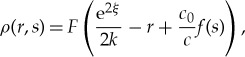
where 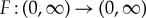is continuously differentiable and non-decreasing, the analogue of the pressure function (2.3) is given, where and , by

(b). Exact solution: internal waves

Following initial work in [18] describing a Gerstner-like internal wave as part of a two-layer hydrostatic model, Constantin successfully derived a physically complex multi-layered, non-hydrostatic model for internal waves in [19], a schematic for which is given below.

The internal wave propagates at the thermocline, denoted η₀, and it is assumed that the wave motion is predominant in the layer labelled M(t); the L(t) layer denotes the upper near-surface region of the ocean which is primarily influenced by the effects of the wind, and where the wave motion is a small perturbation of the ocean dynamics. The generation mechanism for the internal wave is a stratification jump across the thermocline, with the fluid having a constant density ρ₀ in the region above the thermocline η₀, and a constant density ρ₊>ρ₀ beneath the thermocline—indicative values for the density difference in the equatorial region are (ρ₊−ρ₀)/ρ₀≈4×10⁻³. The fluid domain lying beneath the thermocline is divided into three separate regions, which transitions the fluid motion from that induced by the propagation of the thermocline to a motionless abyssal deep-water region. In order to successfully implement this multi-layered model, the continuity of the pressure is maintained across each interface.

In the deep motionless fluid layer, define η₂(x,y,t)=−D+(β/4Ω)y² for some fixed equatorial depth D>0. In the region below η₂(x,y,t), the fluid is in the hydrostatic state u=v=w=0 with the pressure given by P(x,y,z,t)=P₀−ρ₊gz for z≤−D+(β/4Ω)y², where P₀ and D are constants. In the transitional layer, define η₁(x,y,t)=−d+(β/4Ω)y² for some fixed equatorial depth d<D. In the region between z=η₂(x,y,t) and z=η₁(x,y,t), we take v=w=0 and the horizontal component of particle velocity u is given by

with the appropriate pressure function prescribed by

Note that the pressure P and the velocity u are continuous across the interface z=η₂(x,y,t). With z=η₀(x,y,t) representing the wave propagating at the thermocline, in the region η₁(x,y,t)<z<η₀(x,y,t) the uniform flow is given by u=c and v=w=0, with the resulting pressure defined as

Finally, in the layer M(t) above the thermocline the wave-like solution is given by

2.8

with the notation as in the surface wave solution (2.2). For every fixed value of s∈[−s₀,s₀], we require r∈[r₀(s),r₊(s)], where the choice r=r₀(s)>0 defines the thermocline z=η₀(x,y,t) at the latitude y=s, while r=r₊(s)>r₀(s) prescribes the interface z=η₊(x,y,t) separating L(t) and M(t) at the same latitude. An indicative value for (r₊−r₀) is 60 m, cf. [19,41]. The parameter d₀>0 is determined by specifying that [d₀−r₀(0)] is the mean depth of the thermocline at the equator, where r₀(0)>0 is the unique choice of r which prescribes the thermocline at the equator. The wave motion in M(t) induced by the propagation of the thermocline, as described by the solution (2.8), is equatorially trapped for f(s) given by

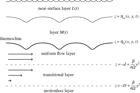
In the course of deriving this complex multi-layered solution, a dispersion relation is obtained for the speed c of the wave propagating along the thermocline which takes the form

2.9

resulting in an eastward-propagating wave. It is clear from the form of (2.9) that the density differential between fluid layers is the major driving force behind wave propagation at the thermocline, and without it c=0 and no such wave would exist. Note that in Gerstner's wave the amplitude of wave oscillations decreases as we descend in the fluid, which is the reverse of the present setting whereby the amplitude decreases exponentially as we ascend above the thermocline. Akin to the surface waves described in [17,39], the introduction of a depth-invariant current was successfully achieved for the internal wave model described in [48].

(c). Some ‘non-traditional’ equatorial β-plane approximations

In this section, two ‘non-traditional’ approximation models are presented for which Gerstner-like solutions also exist. The first modification of the traditional β-plane model incorporates the effects of the commonly neglected centripetal forces, whereas the second aims to retain artefacts of the geometry of the Earth's curvature by way of incorporating a gravitational correction term into the standard β-tangent plane model. While both models are interesting in themselves from a non-traditional approximation perspective, it is quite surprising, given their additional structural properties, that both modifications of the β-plane admit Gerstner-like solutions of the form (2.2). An interesting consequence of both structural modifications is that, compared to §2a above, the additional terms they contribute to the standard β-plane approximation play a central role in facilitating the admission of a wide range of both following and adverse depth-invariant underlying currents in the solution (2.2).

(i). Centripetal forces

In an oceanographic context, centripetal forces are typically neglected as they are relatively much smaller (∼O(Ω²)) than Coriolis terms (∼O(Ω)), where Ω=7.3×10⁻⁵ rad s⁻¹ is the (constant) rotational speed of the Earth. In [38], it was shown that retaining these terms in (1.1) and taking an appropriate tangent-plane approximation leads to the following modified β-equation:

2.10

As distinct from (2.1a), when the fluid motion prescribed by the modified β-plane governing equations (2.10) is still, and the pressure is constant at the free surface, the free surface is a geoid. Since then

throughout the fluid (u=v=w=0), the free-surface geoid is given by

because Ω²R≈3×10⁻² m s⁻²≪g≈9.8 m s⁻². The above distortion from a constant value of z corresponds to a free surface following the curvature of the Earth away from the equator, as the curved surface of the Earth drops below the tangent plane at the equator—this is consistent with, and indeed a consequence of, the β-plane approximation. Remarkably, it can be shown that the solution (2.2) satisfies the modified equations (2.10), with some variations: f(s) is now defined by

where 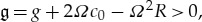with the inequality motivated by physical considerations (since g/2Ω≈6.7×10⁴ m s⁻¹, ΩR/2≈2.33×10² m s⁻¹).

Proposition 2.1 —

[38] The fluid motion prescribed by (2.2) represents an exact solution of the governing equations (2.10) if the underlying current c₀ satisfies

2.11

Henceforth, such values of c₀ will be referred to as ‘physically plausible’. The free surface z=η(x,y,t) is implicitly prescribed at the equator (y=s=0) by setting r=r₀ in (2.2), and for any other fixed latitude s∈[−s₀,s₀], whenever (2.11) holds, there exists a unique value r(s)<r₀ which implicitly prescribes the free surface z=η(x,s,t) by way of setting r=r(s) in (2.2).

Regarding the dispersion relation for the wave described by (2.2) for (2.10), if c₀=c, then 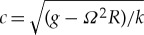: for sufficiently large wavenumbers k (corresponding to sufficiently small wavelengths L), the magnitude of the underlying current c₀ given by this relation may, in principle, be physically attainable, and furthermore it does not contravene the bound given by (2.11). This dispersion relation is a perturbation of the standard Gerstner wave (and deep-water gravity water wave) dispersion relation by additional Coriolis terms which are attributable to the centripetal force. Indeed, the potential balance between the wave phase speed and the adverse current prescribed by c=c₀ is a curious phenomenon which is unique to the modified β-plane formulation (2.10) as it is expressly prohibited by the absence of centripetal terms for the standard model (2.1a). In the more general scenario with c₀≠c, we have

which features contributions from the Coriolis force, the centripetal force and the underlying current. Ignoring the effects of the Earth's rotation (letting ), we recover the standard expression for the deep-water gravity water wave (and Gerstner wave) dispersion relation, namely . Surface waves with wavelengths of 300 m, propagating at speeds of about 22 m s⁻¹, are common in the Pacific—see the discussion in [17]; the corresponding value of the speed predicted by the dispersion relation is, therefore, quite accurate.

(ii). Gravity correction term

The second modified β-plane approximation we consider was derived in [49]. This non-traditional approximation was motivated by the fact that, from a mathematical modelling perspective, an appreciable level of mathematical detail and structure must be lost as a result of the ‘flattening out’ of the Earth's surface which follows from the standard β-plane approximation. An approach which retains some artefacts of the geometry of the Earth's curvature by way of incorporating a gravitational correction term into the standard β-tangent plane model is as follows. We now neglect centripetal terms in (1.1), and in considering the form that the gravitational body force F takes following the linearization procedure, we accommodate a correction term which incorporates the deviation of the tangent plane from the Earth's curved surface. We consider the point P in the figure below, and note that its distance from the Earth's centre O is 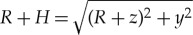where the plane is aligned with the x-coordinate.

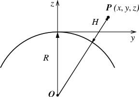
As R is significantly larger than both y and z, we approximate the gravitational potential at P by

The associated gravitational field is , and equations (1.1) reduce to

2.12

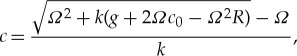
where the gy/R term is the gravitational correction term which arises when we accommodate the direction that gravity acts in for the tangent β-plane model. As

2.13

for all physically plausible values of c₀, it can be shown that (2.2) represents a solution (with ) to (2.12) with

Theorem 2.1 —

[49] For all physically plausible (such that (2.13) holds) values of the mean zonal current c₀, the fluid motion prescribed by (2.2) is an exact solution of the governing equations (2.12). This solution represents three-dimensional, nonlinear geophysical wave–current interactions; the wave terms are equatorially trapped steady periodic waves, propagating zonally eastward with constant wave phase speed c, with insignificant motion at great depths.

As in the previous section, when the fluid motion prescribed by (2.12) is at rest, the free surface is a non-flat geoid, with constant pressure, given in this instance by z=P_atm/ρg−y²/2R.

3. Global validity of exact solutions

While it can be shown by direct computations that the exact solutions described in the previous section satisfy the relevant governing equations (2.1a), (2.10) or (2.12), for appropriately defined pressure distribution functions, it is also necessary to provide a rigorous mathematical justification that the prescribed flow is dynamically possible. Proving that the mapping (2.2) is a global diffeomorphism between the Lagrangian labelling variables and the fluid domain ensures that it is possible to have a three-dimensional, nonlinear motion of the entire fluid body described by (2.2), characterizing wave–current interactions, whereby fluid particles never collide, and furthermore they encompass the entire infinite fluid region beneath the free-surface interface.

We describe briefly the approach which was used in [49] to establish the global validity of (2.2) in solving (2.12); other geophysical scenarios were addressed in [50,51]. Firstly, from examining its Jacobian matrix, and applying the inverse function theorem, it can be proved that the mapping (2.2) represents a local diffeomorphism from the Lagrangian variables to the fluid domain. Additional analytical considerations establish that it is, in fact, globally injective. To complete the proof, as was first implemented in [3] for Gerstner's wave, we employ the following degree-theoretical result, the invariance of domain theorem [52,53], which we state as Theorem 3.1.

Theorem 3.1 —

If is open and is a continuous one-to-one mapping, then is a homeomorphism. Furthermore, we have .

Putting all these components together leads to the following result:

Theorem 3.2 —

[49] The mapping (2.2) is a global diffeomorphism between the Lagrangian labelling variables and the infinite fluid domain bounded above by the free-surface interface z=η(x,y,t). For r₀<0, the free surface has a smooth profile, and in the limiting case r₀=0 the surface is smooth except when s=0, in which case it is piecewise smooth with upward cusps.

4. Hydrodynamical stability analysis

Hydrodynamical stability examines how an infinitesimal perturbation of the background flow evolves, as time progresses, for a given fluid motion [54]. The issue of hydrodynamic stability is important for numerous reasons. Physically, unstable flows cannot be observed in practice because they are rapidly destroyed by any minor perturbations or disturbances. From a mathematical viewpoint, establishing the hydrodynamical stability or instability of a flow is extremely difficult, in general, given the intractability of the underlying governing equations of motion.

The short-wavelength instability method, which was independently developed by the authors of [55–57], examines the evolution of a localized and rapidly varying infinitesimal perturbation represented at time t by the wave packet

4.1

Here, X=(x,y,z), Φ is a scalar function, and at t=0 we have Φ(X,ξ₀,b₀,0)=X⋅ξ₀, and b(X,ξ₀,b₀,0)=b₀(X,ξ₀). The normalized wavevector ξ₀ is subject to the transversality condition ξ₀⋅b₀=0, and b₀ is the normalized amplitude of the short-wavelength perturbation of the flow which has the velocity field U(X)≡(u v w)^T(x,y,z). Then, the evolution in time of X, of the perturbation amplitude b, and of the wavevector ξ=∇Φ, is governed at the leading order in the small parameters ε and δ by the system of ordinary differential equations

4.2

with initial conditions X(0)=X₀, ξ(0)=ξ₀, b(0)=b₀. Here, (∇U)^T is the transpose of the velocity gradient tensor and, for the system defined by (2.2), L=L(X) is given by

The instability criterion, for Lagrangian flows for which X(0)=X₀, is determined by the exponent

If Λ(X₀)>0 for a given perturbation, then particles become separated at an exponential rate and the flow is unstable; this provides us with a criterion to establish the instability of a flow.

For certain solutions which have an explicit Lagrangian formulation, it transpires that the short-wavelength instability analysis is remarkably elegant, and the criteria for instability assume a tangible and explicit formulation in terms of the wave steepness (2.6). In the context of the solution (2.2) describing nonlinear wave–current interactions, the short-wavelength instability method was employed to prove the following result.

Proposition 4.1 —

[45] The equatorial waves propagating eastward over a constant underlying current, as prescribed by (2.2), are unstable to short-wavelength perturbations if the steepness of the wave

4.3

We note from (4.3) that an adverse current with c₀>0 favours instability in the sense that the steepness threshold is decreased for the wave to be unstable, compared to the case without current. Conversely, this threshold is increased by a following current with c₀<0. On letting the right-hand side of (4.3) reduces to , which is the threshold value of the instability criterion for Gerstner's gravity water wave established in [58]. In the setting of no underlying current, c₀=0, the above result reduces to the instability criterion originally established for geophysical surface waves in [59]. We note that further instability results were established in [60–62] for Gerstner-like geophysical surface waves in various settings, such as edge waves, Pollard's solution and the f-plane. A result establishing instability for internal waves was derived in [63].

5. Mean flow properties

The question of determining the fluid drift induced by the propagation of surface water waves is a fascinating, and highly complex, issue which has been considered dating back to the times of Stokes. Longuet-Higgins [64] characterized key features of the mean fluid drift velocity, or so-called Stokes’ drift velocity, in terms of the mean Eulerian flow velocity and the mean Lagrangian flow velocity, whereby Lagrange = Euler + Stokes. Determining the mean fluid flow velocities remains a highly complex and intricate issue from a theoretical, and experimental [9,10], viewpoint. However, as the form of (2.2) is explicit in terms of Lagrangian variables, it transpires that the solution (2.2) is quite amenable to an analysis of its mean flow velocities and related mass transport [19,59]. The presence of a constant underlying current term is a significant complicating factor for the analysis of (2.2), undertaken in [46], and this is what we describe briefly.

The mean Lagrangian flow velocity (also known as the mass-transport velocity [64]) at a point in the fluid domain is the mean velocity over a wave period of a marked fluid particle which originates at that point. For (2.2), the average horizontal velocity u is

5.1

It is immediately apparent that the mean Lagrangian flow velocity is either westwards or eastwards, depending on the sign of c₀. When c₀=0, the mean Lagrangian velocity is zero, which concurs with the result of [59], and in this light the form of the mean Lagrangian flow velocity above is not particularly surprising considering the explicit manner in which c₀ appears in the expression for the Lagrangian velocity (2.2). The expression for the mean Lagrangian velocity is independent of both the latitude s and the location from where the fluid parcel originates.

In the Eulerian setting, matters are greatly complicated by the presence of the underlying current. The mean Eulerian flow velocity at a fixed point in the fluid domain, at any fixed depth beneath the wave trough, is the Eulerian fluid velocity at that fixed point averaged over a wave period. In the case of the velocity field (2.2), the mean Eulerian flow velocity may be computed by taking the mean of the horizontal velocity. Letting z=z₋(s_*) denote the vertical position of the wave trough level, we fix a depth z=z₀<z₋(s_*). The depth z=z₀ is characterized in terms of Lagrangian variables, using (2.2c), by the equation

5.2

where we denote by r=R(q−ct;s_*,z₀) the functional relationship induced by relation (5.2) between the otherwise independent variables r and q, as follows from the implicit function theorem. In [46], it is shown that the mean Eulerian velocity is given by the relation

5.3

with ξ(r,s)=k(r−f(s)) and θ(q,t)=k(q−ct). A non-zero depth-invariant current c₀ adds a significant complicating factor to expression (5.3), and in particular the sign (and hence direction) of the mean Eulerian velocity is not easily discernible from the above expression in general. Nevertheless, depending on the size and direction of the current c₀, we may obtain estimates which determine the direction of the mean Eulerian velocity following from the inequalities

5.4

For c₀>0, an adverse current, we must have 0<c₀<c e^2kr₀<c from (2.5). As ξ≤kR<kr₀<0, for all latitudes s and depths z₀<z₋(s), the mean Eulerian flow velocity is in the range

5.5

That the mean Eulerian flow is westward for an adverse current is not surprising, because in the absence of the current, the mean Eulerian flow is westward in any case (cf. [59]).

The case when c₀ is non-positive, c₀≤0, represents a following current. In this case, the influence that the current has on the mean Eulerian flow in (5.3) is even more complex and difficult to discern, and it is not possible to determine its effect directly from expression (5.3). However, it can be deduced that the mean Eulerian velocity (5.3) is westward, that is 〈u〉_E(s_*,z₀)<0, if

5.6

In the absence of an underlying current, that is when c₀=0, condition (5.6) always holds and so the resulting mean Eulerian velocity is always in the westerly direction, an observation which accords with [59]. The mean Eulerian flow (5.3) is eastward, 〈u〉_E(s_*,z₀)>0, if

5.7

The Stokes drift (or mean Stokes) velocity U^S(z₀), defined (cf. [9,59,64]) by the relation

takes the form

For an adverse current, c₀≥0, it follows from (2.5) that

Therefore, for c₀≥0, the Stokes drift is eastward throughout the fluid domain. In the case of a following current, c₀<0, the expression for Stokes drift is altogether more complicated and intractable. Nevertheless we remark that, for c₀<0, if the magnitude of the current is such that (5.7) holds, then the Stokes drift must be westward.

We note that an analysis of flow properties for geophysical internal waves in the absence of a current (as described in §2b) was performed in [19], and in the presence of a depth-invariant current a similar approach to that outlined above was undertaken in [65].

6. Conclusion

In this paper, we have surveyed equatorial models for GFD, in the form of both traditional and non-traditional β-plane approximations, which have recently yielded exact and explicit Gerstner-like solutions representing nonlinear three-dimensional water waves. These waves propagate at the free surface, and along the internal theormocline, and we have shown how a depth-invariant mean current may be incorporated into the wave-field kinematics. Owing to their rarity, the existence of exact finite-amplitude solutions to the water wave problem is remarkable. Aside from possessing an inherent mathematical elegance, this review outlines how Gerstner-like solutions have proved to be surprisingly adaptable in modelling a variety of geophysical scenarios. Furthermore, we have surveyed how these solutions are naturally suited to an intricate mathematical analysis of the physical flow properties induced by the nonlinear waves, and wave–current interactions, that they prescribe. With regard to future explorations, we remark that, in general, exact solutions play an important role in the study of water waves, as many apparently intangible wave motions can be obtained as perturbations of these solutions. As such, the solutions surveyed may represent a first step in generating solutions prescribing more physically complex flows by way of employing perturbative or asymptotic considerations.

Data accessibility

This article has no additional data.

Competing interests

The author declares that he has no competing interests.

Funding

The author acknowledges the support of the Science Foundation Ireland (SFI) research grant no. 13/CDA/2117. This work was supported by EPSRC grant no. EP/K032208/1.

References

- 1.Constantin A. 2001. On the deep water wave motion. J. Phys. A 34, 1405–1417. ( 10.1088/0305-4470/34/7/313) [DOI] [Google Scholar]
- 2.Constantin A. 2011. Nonlinear water waves with applications to wave–current interactions and tsunamis. CBMS-NSF Conference Series in Applied Mathematics, vol. 81 Philadelphia, PA: SIAM. [Google Scholar]
- 3.Henry D. 2008. On Gerstner's water wave. J. Nonlinear Math. Phys. 15, 87–95. ( 10.2991/jnmp.2008.15.S2.7) [DOI] [Google Scholar]
- 4.Constantin A. 2006. The trajectories of particles in Stokes waves. Invent. Math. 166, 523–535. ( 10.1007/s00222-006-0002-5) [DOI] [Google Scholar]
- 5.Constantin A. 2012. Particle trajectories in extreme Stokes waves. IMA J. Appl. Math. 77, 293–307. ( 10.1093/imamat/hxs033) [DOI] [Google Scholar]
- 6.Constantin A, Strauss W. 2010. Pressure beneath a Stokes wave. Commun. Pure Appl. Math. 53, 533–557. ( 10.1002/cpa.20299) [DOI] [Google Scholar]
- 7.Henry D. 2008. On the deep-water Stokes flow. Int. Math. Res. Not. 22, 071 ( 10.1093/imrn/rnn071) [DOI] [Google Scholar]
- 8.Lyons T. 2014. Particle trajectories in extreme Stokes waves over infinite depth. Discrete Contin. Dyn. Syst. 34, 3095–3107. ( 10.3934/dcds.2014.34.3095) [DOI] [Google Scholar]
- 9.Monismith SG, Cowen EA, Nepf HM, Magnaudet J, Thais L. 2007. Laboratory observations of mean flow under surface gravity waves. J. Fluid Mech. 573, 131–147. ( 10.1017/S0022112006003594) [DOI] [Google Scholar]
- 10.Weber JEH. 2011. Do we observe Gerstner waves in wave tank experiments? Wave Motion 48, 301–309. ( 10.1016/j.wavemoti.2010.11.005) [DOI] [Google Scholar]
- 11.Constantin A, Monismith SG. 2017. Gerstner waves in the presence of mean currents and rotation. J. Fluid Mech. 820, 511–528. ( 10.1017/jfm.2017.223) [DOI] [Google Scholar]
- 12.Dubreil-Jacotin M-L. 1932. Sur les ondes de type permanent dans les liquides hétérogènes. Atti Accad. Naz. Lincei, Mem. Cl. Sci. Fis., Mat. Nat. 15, 814–819. [Google Scholar]
- 13.Constantin A. 2001. Edge waves along a sloping beach. J. Phys. A 34, 9723–9731. ( 10.1088/0305-4470/34/45/311) [DOI] [Google Scholar]
- 14.Mollo-Christensen E. 1979. Edge waves in a rotating stratified fluid, an exact solution. J. Phys. Ocean. 9, 226–229. ( 10.1175/1520-0485(1979)009%3C0226:EWIARS%3E2.0.CO;2) [DOI] [Google Scholar]
- 15.Stuhlmeier R. 2011. On edge waves in stratified water along a sloping beach. J. Nonlinear Math. Phys. 18, 127–137. ( 10.1142/S1402925111001210) [DOI] [Google Scholar]
- 16.Yih CS. 1966. Note on edge waves in a stratified fluid. J. Fluid Mech. 24, 765–767. ( 10.1017/S0022112066000983) [DOI] [Google Scholar]
- 17.Constantin A. 2012. An exact solution for equatorially trapped waves. J. Geophys. Res.: Oceans 117, C05029 ( 10.1029/2012JC007879) [DOI] [PMC free article] [PubMed] [Google Scholar]
- 18.Constantin A. 2013. Some three-dimensional nonlinear equatorial flows. J. Phys. Oceanogr. 43, 165–175. ( 10.1175/JPO-D-12-062.1) [DOI] [Google Scholar]
- 19.Constantin A. 2014. Some nonlinear, equatorially trapped, nonhydrostatic internal geophysical waves. J. Phys. Oceanogr. 44, 781–789. ( 10.1175/JPO-D-13-0174.1) [DOI] [Google Scholar]
- 20.Cushman-Roisin B, Beckers J-M. 2011. Introduction to geophysical fluid dynamics: physical and numerical aspects. Waltham, MA: Academic Press. [Google Scholar]
- 21.Gill A. 1982. Atmosphere–ocean dynamics. New York, NY: Academic Press. [Google Scholar]
- 22.Vallis GK. 2006. Atmospheric and oceanic fluid dynamics. Cambridge, UK: Cambridge University Press. [Google Scholar]
- 23.Constantin A, Johnson RS. 2016. Current and future prospects for the application of systematic theoretical methods to the study of problems in physical oceanography. Phys. Lett. A 380, 3007–3012. ( 10.1016/j.physleta.2016.07.036) [DOI] [Google Scholar]
- 24.Constantin A, Johnson RS. 2015. The dynamics of waves interacting with the Equatorial Undercurrent. Geophys. Astrophys. Fluid Dyn. 109, 311–358. ( 10.1080/03091929.2015.1066785) [DOI] [Google Scholar]
- 25.Constantin A, Johnson RS. 2016. An exact, steady, purely azimuthal equatorial flow with a free surface. J. Phys. Oceanogr. 46, 1935–1945. ( 10.1175/JPO-D-15-0205.1) [DOI] [Google Scholar]
- 26.Constantin A, Johnson RS. 2016. An exact, steady, purely azimuthal flow as a model for the Antarctic Circumpolar Current. J. Phys. Oceanogr. 46, 3585–3594. ( 10.1175/JPO-D-16-0121.1) [DOI] [Google Scholar]
- 27.Constantin A, Johnson RS. 2017. A nonlinear, three-dimensional model for ocean flows, motivated by some observations of the Pacific Equatorial Undercurrent and thermocline. Phys. Fluids 29, 056604 ( 10.1063/1.4984001) [DOI] [Google Scholar]
- 28.Johnson RS. 2017. Application of the ideas and techniques of classical fluid mechanics to some problems in physical oceanography. Phil. Trans. R. Soc. A 376, 20170092 ( 10.1098/rsta.2017.0092) [DOI] [PubMed] [Google Scholar]
- 29.Ionescu-Kruse D. 2015. An exact solution for geophysical edge waves in the β-plane approximation. J. Math. Fluid Mech. 17, 699–706. ( 10.1007/s00021-015-0233-6) [DOI] [Google Scholar]
- 30.Matioc A-V. 2012. An exact solution for geophysical equatorial edge waves over a sloping beach. J. Phys. A 45, 365501 ( 10.1088/1751-8113/45/36/365501) [DOI] [Google Scholar]
- 31.Matioc A-V. 2013. Exact geophysical waves in stratified fluids. Appl. Anal. 92, 2254–2261. ( 10.1080/00036811.2012.727987) [DOI] [Google Scholar]
- 32.Hsu H-C. 2015. An exact solution for equatorial waves. Monatsh. Math. 176, 143–152. ( 10.1007/s00605-014-0618-2) [DOI] [Google Scholar]
- 33.Henry D. 2015. Internal equatorial water waves in the f-plane. J. Nonlinear Math. Phys. 22, 499–506. ( 10.1080/14029251.2015.1113046) [DOI] [Google Scholar]
- 34.Henry D. 2016. Exact equatorial water waves in the f-plane. Nonlinear Anal. Real World Appl. 28, 284–289. ( 10.1016/j.nonrwa.2015.10.003) [DOI] [Google Scholar]
- 35.Kluczek M. 2017. Equatorial water waves with underlying currents in the f-plane approximation. Appl. Anal. 14pp ( 10.1080/00036811.2017.1343466) [DOI] [Google Scholar]
- 36.Rodríguez-Sanjurjo A. 2017. Internal equatorial water waves and wave–current interactions in the f-plane. Monatsh. Math. 17pp ( 10.1007/s00605-017-1052-z) [DOI] [Google Scholar]
- 37.Pollard RT. 1970. Surface waves with rotation: an exact solution. J. Geophys. Res. 75, 5895–5898. ( 10.1029/JC075i030p05895) [DOI] [Google Scholar]
- 38.Henry D. 2016. Equatorially trapped nonlinear water waves in a β-plane approximation with centripetal forces. J. Fluid Mech. 804, R1 ( 10.1017/jfm.2016.544) [DOI] [Google Scholar]
- 39.Henry D. 2013. An exact solution for equatorial geophysical water waves with an underlying current. Eur. J. Mech. B Fluids 38, 18–21. ( 10.1016/j.euromechflu.2012.10.001) [DOI] [Google Scholar]
- 40.Mollo-Christensen E. 1978. Gravitational and geostrophic billows: some exact solutions. J. Atmos. Sci. 35, 1395–1398. ( 10.1175/1520-0469(1978)035%3C1395:GAGBSE%3E2.0.CO;2) [DOI] [Google Scholar]
- 41.Fedorov AV, Brown JN. 2009. Equatorial waves. In Encyclopedia of ocean sciences (ed. J Steele), pp. 3679–3695. San Diego, CA: Academic Press.
- 42.Izumo T. 2005. The Equatorial Current, Meridional Overturning Circulation, and their roles in mass and heat exchanges during the El Niño events in the tropical Pacific Ocean. Ocean Dyn. 55, 110–123. ( 10.1007/s10236-005-0115-1) [DOI] [Google Scholar]
- 43.Johnson GC, McPhaden MJ, Firing E. 2001. Equatorial Pacific Ocean horizontal velocity, divergence, and upwelling. J. Phys. Oceanogr. 31, 839–849. ( 10.1175/1520-0485(2001)031%3C0839:EPOHVD%3E2.0.CO;2) [DOI] [Google Scholar]
- 44.Moum JN, Nash JD, Smyth WD. 2011. Narrowband oscillations in the upper equatorial ocean. Part I: Interpretation as shear instability. J. Phys. Oceanogr. 41, 397–411. ( 10.1175/2010JPO4450.1) [DOI] [Google Scholar]
- 45.Genoud F, Henry D. 2014. Instability of equatorial water waves with an underlying current. J. Math. Fluid Mech. 16, 661–667. ( 10.1007/s00021-014-0175-4) [DOI] [Google Scholar]
- 46.Henry D, Sastre-Gómez S. 2016. Mean flow velocities and mass transport for equatorially-trapped water waves with an underlying current. J. Math. Fluid Mech. 18, 795–804. ( 10.1007/s00021-016-0262-9) [DOI] [Google Scholar]
- 47.Bennett A. 2006. Lagrangian fluid dynamics. Cambridge, UK: Cambridge University Press. [Google Scholar]
- 48.Kluczek M. 2017. Exact and explicit internal equatorially-trapped water waves with underlying currents. J. Math. Fluid Mech. 19, 305–314. ( 10.1007/s00021-016-0281-6) [DOI] [Google Scholar]
- 49.Henry D. 2017. A modified equatorial β-plane approximation modelling nonlinear wave–current interactions. J. Diff. Eq. 263, 2554–2566. ( 10.1016/j.jde.2017.04.007) [DOI] [Google Scholar]
- 50.Rodríguez-Sanjurjo A. 2017. Global diffeomorphism of the Lagrangian flow-map for equatorially-trapped internal water waves. Nonlinear Anal. 149, 156–164. ( 10.1016/j.na.2016.10.022) [DOI] [Google Scholar]
- 51.Sastre-Gomez S. 2015. Global diffeomorphism of the Lagrangian flow-map defining equatorially trapped water waves. Nonlinear Anal. 125, 725–731. ( 10.1016/j.na.2015.06.017) [DOI] [Google Scholar]
- 52.Krawcewicz W, Wu J. 1997. Theory of degrees with applications to bifurcations and differential equations. New York, NY: Wiley-Interscience. [Google Scholar]
- 53.Rothe EH. 1986. Introduction to various aspects of degree theory in banach spaces. Providence, RI: American Mathematical Society. [Google Scholar]
- 54.Drazin PG. 2002. Introduction to hydrodynamic stability. Cambridge, UK: Cambridge University Press. [Google Scholar]
- 55.Bayly BJ. 1987. Three-dimensional instabilities in quasi-two dimensional inviscid flows. In Nonlinear wave interactions in fluids (eds RW Miksad et al.), pp. 71–77. New York: ASME.
- 56.Friedlander S, Vishik MM. 1991. Instability criteria for the flow of an inviscid incompressible fluid. Phys. Rev. Lett. 66, 2204–2206. ( 10.1103/PhysRevLett.66.2204) [DOI] [PubMed] [Google Scholar]
- 57.Lifschitz A, Hameiri E. 1991. Local stability conditions in fluid dynamics. Phys. Fluids 3, 2644–2651. ( 10.1063/1.858153) [DOI] [Google Scholar]
- 58.Leblanc S. 2004. Local stability of Gerstner's waves. J. Fluid Mech. 506, 245–254. ( 10.1017/S0022112004008444) [DOI] [Google Scholar]
- 59.Constantin A, Germain P. 2013. Instability of some equatorially trapped waves. J. Geophys. Res.: Oceans 118, 2802–2810. ( 10.1002/jgrc.20219) [DOI] [PMC free article] [PubMed] [Google Scholar]
- 60.Henry D, Hsu H-C. 2015. Instability of equatorial water waves in the f-plane. Discrete Contin. Dyn. Syst. 35, 909–916. ( 10.3934/dcds.2015.35.909) [DOI] [Google Scholar]
- 61.Ionescu-Kruse D. 2016. Instability of equatorially trapped waves in stratified water. Ann. Mat. Pura Appl. 195, 585–599. ( 10.1007/s10231-015-0479-x) [DOI] [Google Scholar]
- 62.Ionescu-Kruse D. 2016. Instability of Pollard's exact solution for geophysical ocean flows. Phys. Fluids 28, 086601 ( 10.1063/1.4959289) [DOI] [Google Scholar]
- 63.Henry D, Hsu H-C. 2015. Instability of internal equatorial water waves. J. Diff. Eq. 258, 1015–1024. ( 10.1016/j.jde.2014.08.019) [DOI] [Google Scholar]
- 64.Longuet-Higgins MS. 1969. On the transport of mass by time-varying ocean currents. Deep Sea Res. 16, 431–447. ( 10.1016/0011-7471(69)90031-X) [DOI] [Google Scholar]
- 65.Rodrǵuez-Sanjurjo A, Kluczek M. 2016. Mean flow properties for equatorially trapped internal water wave–current interactions. Appl. Anal. 96, 2333–2345. ( 10.1080/00036811.2016.1221943) [DOI] [Google Scholar]
Associated Data
This section collects any data citations, data availability statements, or supplementary materials included in this article.
Data Availability Statement