High-Throughput Analysis of Ovarian Cycle Disruption by Mixtures of Aromatase Inhibitors

Abstract

Background:

Combining computational toxicology with ExpoCast exposure estimates and ToxCast™ assay data gives us access to predictions of human health risks stemming from exposures to chemical mixtures.

Objectives:

We explored, through mathematical modeling and simulations, the size of potential effects of random mixtures of aromatase inhibitors on the dynamics of women's menstrual cycles.

Methods:

We simulated random exposures to millions of potential mixtures of 86 aromatase inhibitors. A pharmacokinetic model of intake and disposition of the chemicals predicted their internal concentration as a function of time (up to 2 y). A ToxCast™ aromatase assay provided concentration–inhibition relationships for each chemical. The resulting total aromatase inhibition was input to a mathematical model of the hormonal hypothalamus–pituitary–ovarian control of ovulation in women.

Results:

Above 10% inhibition of estradiol synthesis by aromatase inhibitors, noticeable (eventually reversible) effects on ovulation were predicted. Exposures to individual chemicals never led to such effects. In our best estimate, $\sim 10\%$ of the combined exposures simulated had mild to catastrophic impacts on ovulation. A lower bound on that figure, obtained using an optimistic exposure scenario, was 0.3%.

Conclusions:

These results demonstrate the possibility to predict large-scale mixture effects for endocrine disrupters with a predictive toxicology approach that is suitable for high-throughput ranking and risk assessment. The size of the effects predicted is consistent with an increased risk of infertility in women from everyday exposures to our chemical environment. https://doi.org/10.1289/EHP742

Introduction

Concern is growing worldwide over the negative human health and environmental impacts of chemical pollutants that can interfere with the production, metabolism, and action of natural hormones, the so-called endocrine-disrupting chemicals (EDCs). In humans, EDCs have been linked to reproductive disorders (Sweeney et al. 2015), abnormal or delayed development in children (Schug et al. 2015), changes in immune function (Rogers et al. 2013), and cancer (Birnbaum and Fenton 2003). Exposure to mixtures of EDCs may result in effects that can depart from mere summation (Kortenkamp 2007), and human subgroups (e.g., women) may not be sufficiently protected against mixtures of EDCs by current regulatory limits (Kortenkamp 2014).

Each menstrual cycle in women involves hormonal regulation of follicular growth and maturation resulting in ovulation of a single oocyte (Falcone and Hurd 2013). The cycle is controlled by coordinated stimulations and inhibitions along the hypothalamus–pituitary–ovarian axis. Gonadotropin-releasing hormone (GnRH), secreted by the hypothalamus, stimulates the secretion of gonadotropins [follicle-stimulating hormone (FSH) and luteinizing hormone (LH)] by the anterior pituitary gland. Those hormones, in turn, regulate the secretion of ovarian hormones, such as estradiol (E2) or progesterone (P4). Exposures to EDCs that interfere directly or indirectly with any of these hormones can eventually induce infertility or other pathological outcomes. Aromatase is critical because it irreversibly converts testosterone to E2 and androstenedione to estrone, maintaining the dynamic balance between androgens and estrogens.

The objective of the present work was to explore predictively the effects of exposure to large-scale (i.e., potentially real-life) mixtures of aromatase inhibitors on the dynamics of menstrual cycling in women. We input exposure estimates from ExpoCast (Wambaugh et al. 2013) and biological effect data from ToxCast™ (Dix et al. 2007) to coupled pharmacokinetic (PK) and ovarian cycle models; this provided a quantitative mechanistic link between exposure to mixtures of EDCs and their potential adverse effects on the menstrual cycle in women. We compared the expected effects of exposures to single EDCs, as is usually considered by risk assessment provisions in different regulations, with estimated effects of cumulative and concurrent exposures.

Methods

Workflow Overview

The overall computational workflow is pictured in Figure S1. Briefly, after selecting the chemicals of interest, we sampled millions of random mixtures of chemicals using the exposure estimates provided by ExpoCast (Wambaugh et al. 2013). Both constant and time-varying exposure scenarios of an adult woman were considered. A pharmacokinetic model of intake and disposition was then used to estimate the blood concentration (over 2 y) for each chemical present in each mixture. The resulting aromatase activity inhibition was estimated using the Hill's dose–response model parameters provided by ToxCast™ (Dix et al. 2007). A mathematical model of the hypothalamus–pituitary–ovarian hormonal events [based on a study by Chen and Ward (2014)] was used to predict the levels of E2, P4, and other quantities characterizing the ovarian cycle, for a reference cycle and following exposure to the mixtures generated. Monte Carlo sampling (Bois et al. 2010) was used to propagate uncertainties in exposure, kinetics, and dose–response relationships up to ovarian cycle perturbation.

Databases, Chemical Selection, and Mixture Sampling

ExpoCast (Wambaugh et al. 2013) provides exposure estimates, with measures of uncertainty, for 1,936 chemicals. Those exposure estimates were obtained using far-field, mass-balance human exposure models (USEtox® and RAIDAR).

In ToxCast™ (11 December 2013 release), the Tox21-aromatase-inhibition assay is a cell-based assay measuring CYP19A1 (aromatase) gene activity via a fluorescent protein reporter gene. Chemicals acting on aromatase mRNA synthesis, degradation, or translation, or on aromatase itself, should give positive results in this assay (Chen et al. 2015). For each chemical x assayed, ToxCast™ provides the geometric mean and standard error for the parameter values $A{C}_{\mathrm{50},x}$ (half-maximal response), $W_x$ (exponent), $B_x$ (baseline value) and $T_x$ (maximum value) of a Hill function fitted to the concentration–inhibition data (scaled using the positive and negative controls' data):

$$\mathrm{\%}Inhibition=B_x+\left(T_x-B_x\right)\frac{C_x^{W_x}}{{AC}_{50,x}^{W_x}+C_x^{W_x}}.$$ [1]

In ToxCast™, 1,102 chemicals are identified as aromatase inhibitors by the Tox21-aromatase-inhibition assay (on MCF-7 human breast cells) with a fitting that “mate basic requirements of Hill model with some minimal confidence in T and B.” Among those, 256 chemicals (matching either by CAS number or by chemical name) also had exposure estimates in ExpoCast. However, cytotoxicity has been shown to induce many false positive results in ToxCast™ (Judson et al. 2016). Of the 256 chemicals mentioned above, we kept only the 86 that had an ${\text{AC}}_{90}$ (90% of maximal response) for aromatase inhibition lower than their cytotoxicity ${\text{AC}}_{10}$ (10% of maximal response) (as measured by the ToxCast™ proliferation decrease assay on T47D human breast cells). The virtual mixtures generated included all of those 86 chemicals.

Exposure Modeling

ExpoCast provided the molecular mass, geometric mean, and lower and upper 95% confidence limits of the exposure rate (milligrams per kilogram per day) for each chemical present in the randomly generated mixtures. For constant exposure modeling over 10 mo, we sampled a rate for each chemical from the corresponding log-normal distribution, but with a standard deviation (SD) scaled by the square root of the number of days of exposure simulated (because a constant exposure rate should be a time average level in that case) and converted it to micromoles per kilogram per minute.

More realistic time-varying exposures over a 2-y period were also modeled [similarly to the report of Bertail et al. (2010)] using exposure windows of random length and intensity. We first sampled the number $n$ of exposure windows for each chemical in the mixture from a scaled exponential distribution (with a rate parameter equal to 5). That yielded on average 145 exposure events over 2 y (median: 100 events, first quartile: 40 events, third quartile: 200 events). The $n$ exposures’ start and end times were sampled uniformly over the 2-y period. The exposure rate during each of the $n$ exposure windows was randomly sampled from the log-normal distribution given by ExpoCast, with an SD scaled by the number of days of the exposure window considered (or unscaled if the exposure lasted less than a day).

To obtain a lower bound on the effect of mixtures, we similarly simulated random nonoverlapping exposures to the 86 EDCs selected (i.e., each person was exposed to the 86 chemicals, in random order, at random times, but to only one chemical at a time).

Pharmacokinetics Modeling

For each chemical in each mixture, a one-compartment PK model was used to estimate its internal concentration (in micromoles) at steady state in the case of constant oral exposure or at any point in time in the case of varying oral exposures. Steady-state internal concentrations for chemical x were calculated as:

$$C_{x,ss}=\frac{F_x\times E_x}{K_{e,x}},$$ [2]

where $F_x$ is the bioavailability of $x$ (unitless), $E_x$ is its exposure rate (in micromoles per kilogram per minute, sampled as indicated above), and $K_{e,x}$ is its total body clearance rate constant (per minute). A body density of 1 was assumed.

For time-varying exposures, internal concentrations were obtained as a function of time by numerical integration of the following differential over a 2-y period (with an initial value set to zero):

$$\frac{\partial C_x}{\partial t}=F_x\times E_x-K_{e,x}\times C_x.$$ [3]

We used quantitative structure-activity relationships (QSAR) to obtain central estimates of $F_x$ and $K_{e,x}$ for each of the 86 aromatase inhibitors considered. The robustness of the prediction was evaluated by examining compounds from the training set similar to the target substances, together with literature data and references.

$F_x$ central estimates were obtained at several oral dose levels and were linearly interpolated between dose levels as needed. Beyond the dose rates of 0.001 to $10\mathrm{mg}/\text{d}$, the $F_x$ value at the closest bound was used.

To take into account the uncertainty affecting the QSAR-estimated PK parameters, we randomly sampled F values from beta distributions (naturally bounded between 0 and 1), with parameters calculated such that the distribution modes corresponded to the interpolated value of $F_x$ with a coefficient of variation (CV) of 20% (for null $F_x$ modes, a and b were set to 1 and 50, yielding a median at 0.01, a first quartile at 0.006, and a third quartile at 0.03, approximately). $K_{e,x}$ values were log-normally sampled with a geometric mean equal to the central estimates obtained by QSAR and a geometric SD corresponding to a factor of 3.

Ovarian Cycle Model

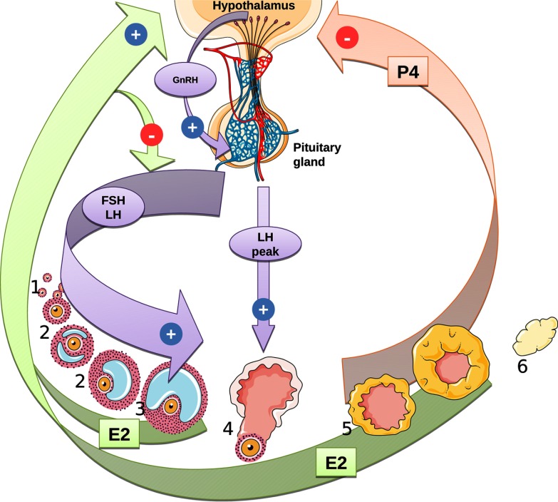
We adapted the menstrual cycle model presented by Chen and Ward (2014). The model describes the inhibitory and stimulatory effects of hormones E2 and P4 on the hypothalamus–pituitary axis in women (Figure 1). The equations and definitions of all parameters used in the model are given in the Supplemental Material (see “Menstrual cycle model equations”; see also Tables S3 and S4). In the original model, E2 and P4 were assumed to be instantaneously in equilibrium between blood and the ovaries. Instead, we described the kinetics of E2 and P4 using differential equations (Equations 15–19 in the Supplemental Material, “Menstrual cycle model equations”). That modification had practically no impact on the time course of the model variables during a normal cycle [equilibrium between blood and ovaries is fast, as assumed by Chen and Ward (2014)], but it allowed us to coherently integrate the dynamic aspect of estradiol synthesis inhibition by EDCs. The three additional parameters (blood and ovarian volumes, ovarian blood flow) were obtained from the literature (see Table S3).

Figure 1.

Regulatory pathways of the human menstrual cycle as implemented in the model. During the follicular phase (1: germ cells; 2: developing follicle; 3: mature follicle; 4: ovulation; 5: corpus luteum formation; 6: corpus luteum degradation), negative feedback by estradiol (E2) reduces follicle-stimulating hormone (FSH) secretion, leading to the selection of one follicle for ovulation. Gonadotropin-releasing hormone (GnRH) secretion is promoted by E2 and inhibited by progesterone (P4), inducing a luteinizing hormone (LH) peak and consecutive ovulation. E2 is mainly produced by follicles and corpus luteum and P4 by corpus luteum.

An additional variable, the ratio of disrupted over basal E2 synthesis rate constants ($E{D}_{CYP\mathrm{19}}$), was introduced to link the internal doses of chemicals in mixtures to aromatase inhibition. $E{D}_{CYP\mathrm{19}}$ was calculated using Hill’s model, parameterized with the chemical-specific values provided by ToxCast™, as a cumulative product of remaining activity for each of the m chemicals of the mixture considered:

$${ED}_{\text{CYP}19}=\prod _{x=1}^{x=m}\left(1-\frac{T_x}{100\left({AC}_{50,x}^{W_x}+C_x^{W_x}\right)}\right).$$ [4]

For constant exposures, $C_x$ was set to the steady-state internal concentrations $C_{x,ss}$. For time-varying exposures, $C_x$ was computed by integration as explained above. The parameter $B_x$ was set to zero because a positive inhibition with no dosage would not make sense. $A{C}_{\mathrm{50},x}$, $W_x$, and $T_x$ values were randomly sampled using the mean and standard error provided by ToxCast™. $A{C}_{\mathrm{50},x}$ was sampled from a log-normal distribution (its logarithm is actually the ToxCast™ fitted value). $W_x$ and $T_x$ were sampled from truncated normal distributions. Truncation was from 0 to 10 for $W_x$ (values beyond 10 would be found for some chemicals for which $W_x$ is poorly identified, but have no biological meaning). Truncation was from 0 to 100 for letrozole's $T_x$ (the positive control). For the other chemicals, truncation was from 0 to 10,000 over $T_x$ for letrozole to properly rescale the ToxCast™ $T_x$ values between 0 and 100.

$E{D}_{CYP\mathrm{19}}$ was entered as an input to the ovarian cycle model, which was then solved to obtain the time profile of its output variables over 2 y of simulated time. For constant exposures, we computed the square root of the sum of the squared Euclidean distances between a reference E2 concentration ($E{D}_{CYP\mathrm{19}}$ set at zero) and the perturbed concentrations (at a fixed set of times) as a summary measure of disruption.

Software Used

The ACD/Labs Percepta platform modules ACD/Oral Bioavailability and ACD/PK Explorer were used for the prediction of oral bioavailability (F) and the total body clearance rate constant ($K_e$), respectively (see Supplemental Material, “PK modules of ACD/Labs”; see also Table S1 and Figures S2 and S3). GNU MCSim v5.6.5 (www.gnu.org/software/mcsim) (Bois 2009) was used to build the ovarian cycle model. R v3.1.1 (R Development Core Team) with the parallel, deSolve, and EnvStats packages was used for database processing, numerical integration of the models, and graphics.

Results

Estimates of Internal Dose

The relationship between constant exposure rates and steady-state internal concentrations for the 86 EDCs considered indicates that exposures ranged from ${10}^{-8}\mathrm{\mu }\text{mole}/\mathrm{kg}/\text{d}$ to ${10}^{-3}\mathrm{\mu }\text{mole}/\mathrm{kg}/\text{d}$ and that the resulting steady-state internal concentrations ranged from ${10}^{-13}\mathrm{\mu }\mathrm{M}$ to ${10}^{-3}\mathrm{\mu }\mathrm{M}$ (see Figure S4). The exposure rates and pharmacokinetic parameters were Monte Carlo sampled as described above. For any single EDC, uncertainty is approximately a factor of 10 for exposures and approximately a factor of 1,000 for the resulting internal concentrations. For time-varying exposures, Figure S5 shows an example of a simulated random 2-y time course of internal concentration for lindane. Such profiles were obtained for each chemical in each simulated mixture.

Cycle Model Behavior

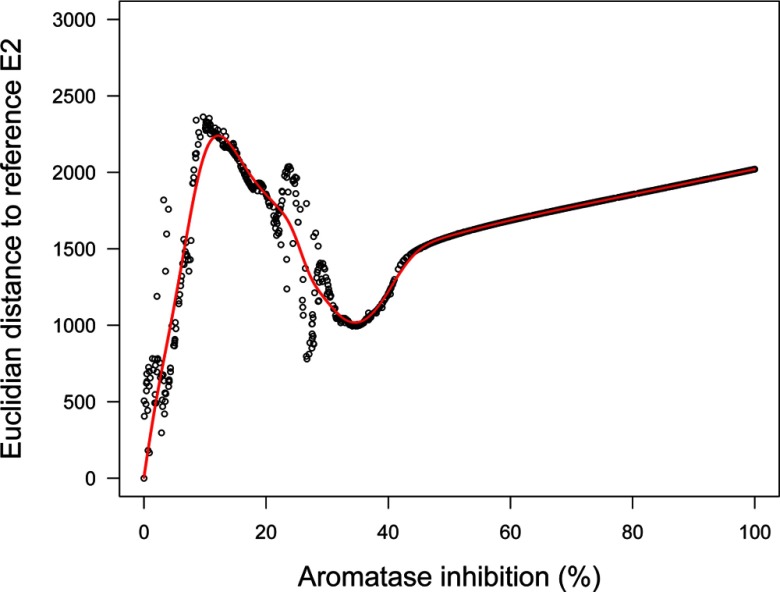
Our implementation of the ovarian cycle model proposed by Chen and Ward (2014) correctly reproduces their results. Human data from McLachlan et al. (1990) and Welt et al. (1999) on LH, FSH, E2, and P4 normal cycles are correctly simulated except for McLachlan FSH data, for which the baseline levels are not well matched. There is a large intra- and inter-subject variability in hormonal levels across women in those data sets (see Figure S6). We took the model-simulated normal cycling of E2 as the “reference cycle” in the following. Constant exposure scenarios result, at steady state, in a constant level of aromatase inhibition. In that case, perturbation depends only on that parameter (according to the model assumptions), so the distance between the perturbed and reference cycles is a useful measure of effect (see Figure 2). As aromatase inhibition increases, cycles become increasingly perturbed and exhibit chaotic features (hence the misalignment of the points in Figure 2). At 5% inhibition (95% of normal aromatase activity), cycles are shortened, baseline levels change little, and peak levels either increase or decrease less than proportionally except for LH. Simply put, the regulations dampen the effect of perturbation. At $\sim 10\%$ inhibition, LH peaks disappear after approximately five cycles, and a major bifurcation in cycle patterns occurs: cycles are further shortened, baseline levels are much increased (doubled for E2 and P4, for example, even though E2 synthesis by aromatase is decreased), and peak levels mostly decreased; E2 distance to normal increases up to a maximum (Figure 2). At higher inhibition levels, the cycles increasingly dampen and disappear completely between 30% and 40% inhibition (see Figures S7–S10). Overall, according to this model, having $\sim 10\%$ constant inhibition of aromatase activity in vivo leads to perturbations of the cycle, which is still under control and should be compatible with normal reproductive function. Beyond 10% inhibition, an actual disruption of the system seems to occur.

Figure 2.

Euclidean distance between an estradiol (E2) normal cycle and a perturbed cycle as a function of aromatase inhibition at steady state. Distance is computed over 2 y based on 7,301 time points (one every 144 min).

Effects of Single Chemicals

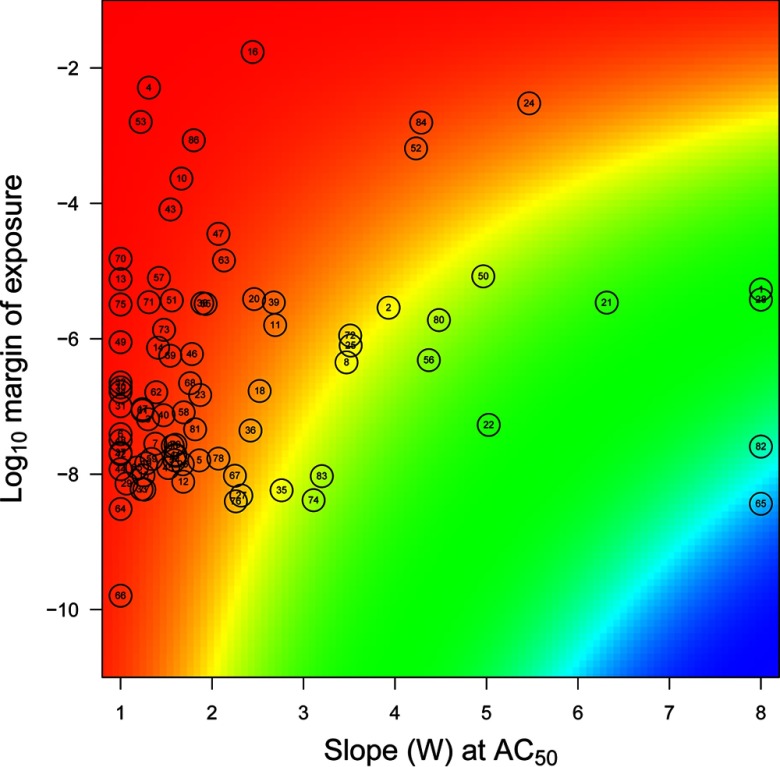
We first simulated 1,000,000 constant exposures to each of the 86 chemicals considered, taken individually. In that case, despite accounting for uncertainty in exposure levels and dose–response parameters, none induced $>1\%$ aromatase inhibition. Hence, none of those chemicals alone was able to induce a significant disruption of the ovarian cycle. Figure 3 places those chemicals on a map with the slope W of the Hill dose–response curve at $A{C}_{\mathrm{50}}$ and the log-margin of exposure as coordinates. The margin of exposure was defined as the ratio of the 97.5th percentile of internal concentrations over $A{C}_{\mathrm{50}}$. The ${\log }_{10}-\text{margins}$ of the chemicals studied ranged from $-10$ to $-1.8$, indicating that for all chemicals, the high end of internal exposure concentrations was at most 1% of $A{C}_{\mathrm{50}}$. In that case, Equation 1 shows that the logarithm of aromatase inhibition is approximately equal to the product of W times the log-margin of exposure. The color background of the map codes for the resulting risk index (i.e., the ${\log }_{10}-\text{inhibitions}$) and ranges from <$-2$ (1%) to approximately $-80$ (${10}^{-78}\%$), much too low to elicit changes in ovarian cycles such as those in Figure 2. Therefore, no effects can be expected from typical exposures to those chemicals when considered alone. Table 1 gives the list of the 10 chemicals for which individual risk is the highest. Note that letrozole is the reference chemical for the Tox21 aromatase inhibition assay, which is consistent with its high rank. The others are found in therapeutic drugs, agrochemicals, food contaminants, consumer products, and other materials.

Figure 3.

Map of the aromatase inhibitors studied over a plane defined by dose–response slope W and log-margin of exposure (see text). Colors vary linearly with powers of 10 of aromatase inhibition resulting from W and margin of exposure combinations, from red (${10}^{-2}$) to blue (${10}^{-80}$). For the chemicals–numbers correspondence, see Table S1.

Table 1.

Top-ranking chemicals according to their individual risk indices. Those chemicals are in the top left corner of Figure 3.

ExpoCast name	CAS number	Risk indexa
Letrozole	112809-51-5	$-2.99$
Estrone	53-16-7	$-3.41$
Fulvestrant	129453-61-8	$-4.30$
Triflumizole	68694-11-1	$-4.81$
2,4,7,9-Tetramethyl-5-decyne-4,7-diol	126-86-3	$-5.11$
n-Methyl-2-pyrrolidone	872-50-4	$-5.49$
Rhodamine 6G	989-38-8	$-5.51$
Anastrozole	120511-73-1	$-6.04$
Fenvalerate	51630-58-1	$-6.05$
Imazalil	35554-44-0	$-6.31$

^a$\text{Risk}\text{index}=W\times {\log }_{10}\left(E_{95}/A{C}_{50}\right)$, where $E_{95}$ is the 95th percentile of the exposure values sampled, W is the Hill exponent, and AC50 the half-maximal response.

Effects of Mixtures of Chemicals

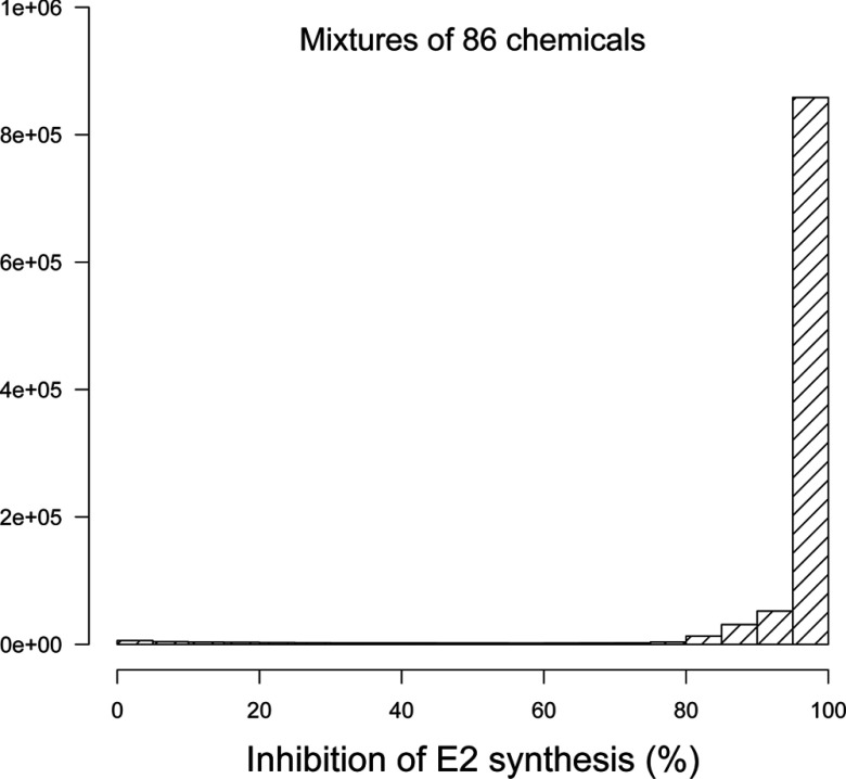
We generated 1,000,000 hypothetical mixtures of the 86 aromatase inhibitors studied and evaluated their global effect on E2 synthesis and the resulting ovarian cycle disruption. Figure 4 shows a histogram of the resulting inhibition levels. Depending on the (random) composition of the mixtures, and given the uncertainties on exposures and effect parameters, responses ranged from 0% to 100% inhibition, but on average were very high. Such inhibition levels may lead to perturbation of the ovarian cycle, according to the model.

Figure 4.

Histogram of the average percent inhibition of estradiol (E2) synthesis by random mixtures ($n=\mathrm{1,000,000}$) of 86 aromatase inhibitors at constant exposure levels.

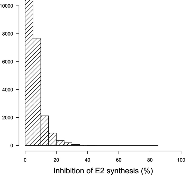
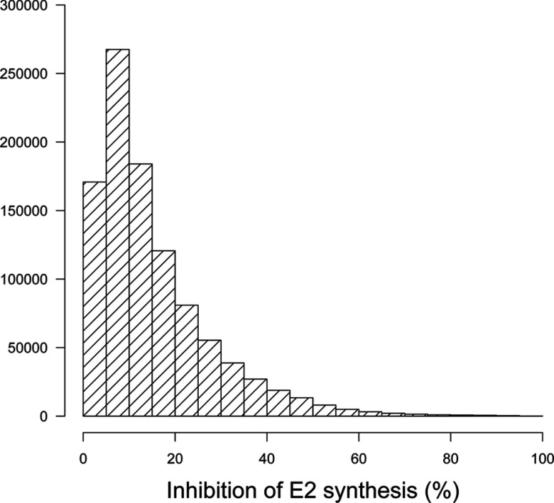
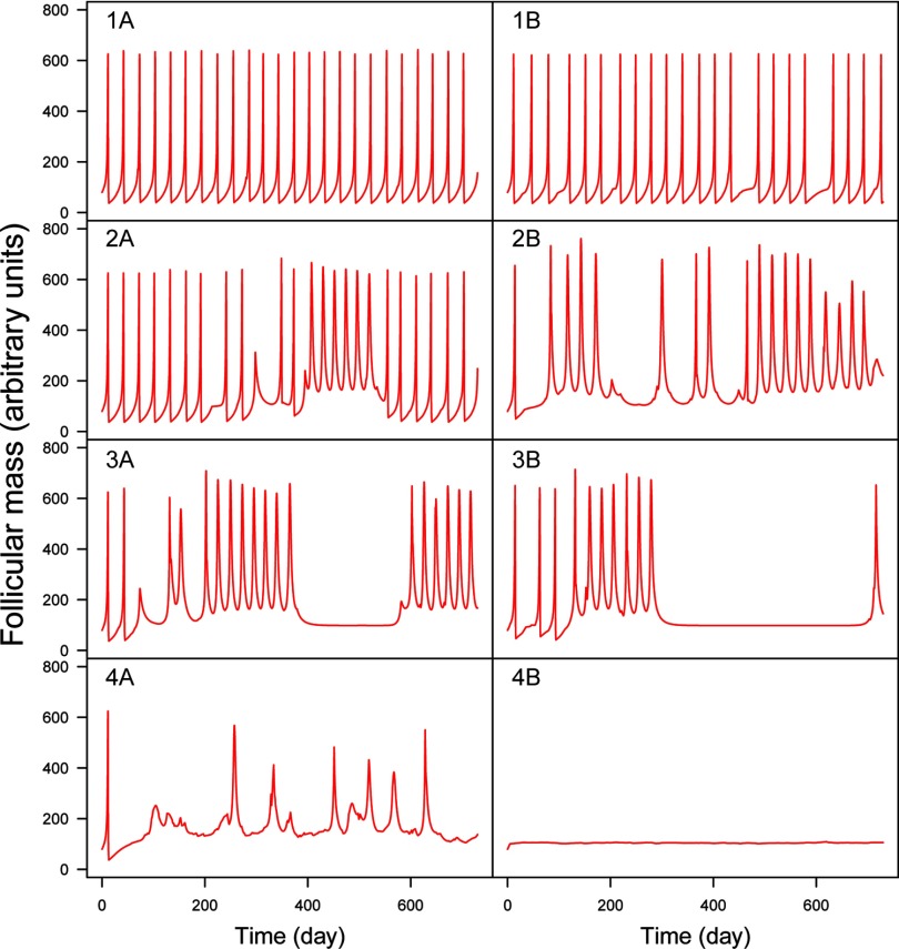
Real-life exposures to chemicals do not usually occur at constant levels. We simulated time-varying exposures (see Figure S5) to investigate the resulting effects on aromatase inhibition and ovarian cycle disruption. To define a lower bound on mixture effects, we first simulated fluctuating levels of exposure to EDCs, but without concomitant exposures to them. Interactions can still occur in that case because of storage in the body or because of persistent effects on the ovarian cycle. Figure 5 shows that only 0.3% of the simulated exposures caused $>10\%$ average aromatase inhibition. The maximum inhibition found was close to 50%. More realistic exposure scenarios do not prohibit concomitant exposures. In that case (Figure 6), the distribution of simulated time-averaged inhibitions is shifted toward greater effects, and average inhibitions $>20\%$ are not uncommon (yet they do not reach the extreme levels observed in Figure 4). Because inhibition changes with time, the distances between normal and perturbed cycles do not follow the pattern shown in Figure 2 (distances can be much larger), and the link between estradiol inhibition and cycle disruption is harder to establish. Examination of the time course of the dominant follicle mass (F) for 1,000 random simulations of mixtures of the 86 chemicals shows that perturbed cycles typically have a baseline shifted up (which may or may not return to normal) and an irregular succession of peaks (corresponding to ovulation) (Figure 7). The 1,000 simulations examined can be classified into four groups. In group 1 (17% of the samples), the cycles are practically normal with no baseline shifts and at most one or two missing ovulations. In group 2 (73% of cases), baseline shifts are always present but without major irregularities in ovulation. Group 3 (7% of cases) has systematic baseline shifts and frequent or prolonged anovulations. Such cycling would clearly impair fertility. In group 4 (3% of cases), disruption is catastrophic or total. Figure S11 shows the corresponding plots for E2 time courses. Judging by these plots, E2 profiles can have a shifted baseline even in normal ovulation profiles, but otherwise, the patterns are rather similar.

Figure 5.

Histogram of the average percent inhibition of estradiol (E2) synthesis by random mixtures ($n=\mathrm{1,000,000}$) of 86 aromatase inhibitors with time-varying nonconcomitant exposures. For visibility, the first histogram bar has been truncated (it represents $\sim \mathrm{90,000}$ simulations). Note: E2, estradiol.

Figure 6.

Histogram of the average percent inhibition of estradiol (E2) synthesis by random mixtures ($n=\mathrm{1,000,000}$) of 86 aromatase inhibitors with time-varying exposures.

Figure 7.

Typical simulated time profiles of dominant follicle mass during time-varying exposures to random mixtures of 86 aromatase inhibitors. Four classes (rows) of increasing disruption are illustrated (see text). Left column: least disrupted profile in its class; Right column: most disrupted. Responses range from regular ovulation (1A) to complete disruption (4B).

Discussion

We linked ToxCast™ data and ExpoCast estimates of exposures to (mixtures of) aromatase inhibitors and estimated their effects on the ovarian cycle in women. To our knowledge, this is the first application of computational toxicology and high-throughput testing to assessment of the combined effects of exposures to a large number of EDCs.

Our approach is predictive, and we had to make many assumptions and simplifications. ToxCast™ and ExpoCast are incomplete, and a full inventory of all the EDCs to which women are exposed is not yet available. Therefore, we were only able to look at a subset of the potential EDCs. We used human exposure estimates reported by Wambaugh et al. (2013), who gave summary statistics for the distribution of exposures to individual chemicals. This information allowed us to take the correspondingly large uncertainty into account via Monte Carlo simulations. However, we cannot differentiate between uncertainty and variability in those exposure estimates, and we cannot identify subgroups of sensitive individuals. We cannot even focus on women, our target population. More sophisticated exposure models (Isaacs et al. 2014) could help in that respect, but they still deal only with single chemicals and provide no data or estimates on coexposures. Depending on age, occupation, socioeconomic status, ethnicity, and health condition, we are exposed to different cocktails of chemicals in our diet, workplace, environment, and so forth (Tornero-Velez et al. 2012). We modeled coexposures by random sampling, either at a constant level or, more realistically, with time-varying exposure profiles and hence with time-varying mixture complexity. That approach is still imperfect, and we had to guess about the distribution of the number of exposure windows, for example. We respected the distribution of population exposure levels documented by ExpoCast, but lacking coexposure information, our estimates might be lower or higher than in reality. Efforts are ongoing to collect relevant data in, for example, the European Total Diet Study (Vin et al. 2014). An analysis of such data (Traoré et al. 2016) shows that among 153 synthetic chemicals studied in seven typical French diets (food associations), three are aromatase inhibitors according to ToxCast™: zearalenone, triadimenol, and lindane. In this regard, mixtures of $\ge 86$ aromatase inhibitors may seem unrealistic, but only food contaminants were studied by Traoré et al. (2016).

We searched for the 86 selected aromatase inhibitors in a database of consumer products marketed in the United States (Gabb and Blake 2016). Briefly, this database was constructed by scraping product information from online retailers and currently contains 53,743 products. Twelve of the 86 aromatase inhibitors were detected in 5,701 products (representing 11% of the products in the database). [It is worth noting that none of the 86 aromatase inhibitors is among the volatile fragrance chemicals detected in consumer products (Steinemann 2015; Steinemann et al. 2011), so aromatase inhibitors are unlikely to be hidden in generic “fragrance” or “flavor” designations on consumer product labels.] Two-way combinations of these chemicals were found in 220 products, and the three-way combination of carminic acid, FD&C blue no. 1, and retinol was found in 3 products. These findings may not seem to indicate a large problem, but it is an incomplete view of combinatorial exposure. Consider that 3,660 of 4,501 makeup products (81%) in the database contain at least one of the aromatase inhibitors evaluated (carminic acid, retinol, and artificial colors are common ingredients in makeup) and that a typical consumer uses several products each day, possibly even several makeup products. This increases the likelihood of combined exposures. In addition, no readily available data address associations for all near- and far-field exposures for the 86 aromatase inhibitors, which are used in industrial or agricultural processes (18), consumer product formulations (12), biocidal applications (38), and pharmaceutical drugs (18). These usage categories are likely to be independent, so focusing on a few known associations would only give partial answers and would underestimate global risk. We are striving for a more extensive picture. To address the potential overestimation of mixture effects when generating purely random associations, we present the results of a very optimistic exposure scenario (with no coexposures at all). This scenario gives a lower bound estimate: 0.3% of exposures would lead to $>10\%$ average aromatase inhibition in women.

ToxCast™ aromatase inhibition data were obtained by exposing cells in vitro. We had no easy way to assess the in vitro kinetics of the substances assayed, and reconstruction methods (Armitage et al. 2014) require input data that we did not have. We assumed that the nominal assay concentrations were those actually experienced by the cells and that equivalent extracellular concentrations in vivo would lead to the same levels of aromatase inhibition. That is a typical assumption, but it is not necessarily correct (Coecke et al. 2013). To obtain extracellular concentrations in vivo, we estimated bioavailability and total clearance with QSAR methods and input them in a simple one-compartment PK model with oral exposure only (even though inhalation or dermal exposures might be more relevant). Again, more sophisticated [physiologically based pharmacokinetic (PBPK)] models and additional PK data would give more precise and more accurate predictions (El-Masri et al. 2016; Wambaugh et al. 2015).

On the effect side, we only considered chemicals for which the ToxCast™ dose–response parameters were estimated with reasonable confidence. This was a conservative choice, and additional chemicals would have been included if more relaxed criteria had been chosen (at the cost of lower confidence in the results). A concern with large databases such as ToxCast™ is the quality assurance for the data provided. Aromatase inhibition may not be the most sensitive toxicity end point, for example, or the action may be due to a burst effect of cytotoxicity (Judson et al. 2016). From the original set of 256 aromatase inhibitors for which we had exposure estimates and ToxCast™ data, 170 were excluded based on cytotoxicity. Those were mostly weak inhibitors (data not shown). For the screen, we kept only the 86 substances that had an aromatase inhibition ${\text{AC}}_{90}$ lower than their cytotoxicity ${\text{AC}}_{10}$ as measured by the ToxCast™ proliferation decrease assay on T47D human breast cells, a cell type similar to the MCF-7 used by the aromatase inhibition assays (Aka and Lin 2012). We preferred that screen to the omnibus z-score criterion, which aggregates cytotoxicity results from different cell types and species. For the remaining 86 substances, we may still have downplayed other types of toxicity. Cytotoxicity, it should be noted, is not a negligible end point, and an evaluation of the cytotoxicity of mixtures would be interesting in its own right.

The evidence provided by ToxCast™ is also not perfectly predictive of in vivo outcomes in humans. For example, the Tox21 aromatase inhibition assay uses the MCF-7 breast cancer cell line, which might not respond as normal ovary cells would. In addition, our model of the ovarian cycle (Chen and Ward 2014) describes only approximately the complex dynamic interactions between ovarian follicular growth and hormonal homeostasis. The hypothalamus and pituitary gland are treated as a single compartment, and the description of the central hormonal controls is simplified. More complex models have been proposed (Hendrix et al. 2014), but they still make many assumptions and do not seem to offer dramatically better performance. In addition, we note that we treated the parameters of the ovarian cycle as constant, when in fact they are affected by both uncertainty and variability in response to EDCs, adding to the tails of the distributions of our results. However, we did not have sufficient information to define statistical distributions for those parameters.

In terms of results, an obvious question is that of the “bad” actors, that is, the chemicals responsible for the predicted effects. The answer is provided by Figure 3 (and partially by the top-ten Table 1) because here, the impact of individual chemicals on aromatase is only conditioned by internal dose and inhibition potency. Figure 3 is a useful prioritization tool. It is rather simple to construct and does not require running the ovarian cycle (the PK model is needed). However, it does not give an answer in terms of magnitude of effect at the subject level. For that, we need the whole-body ovarian cycle model.

One of the consistent features of E2 cycle perturbation that we found is that the baseline (interovulation) levels of E2 tend to increase (to approximately twice the normal level) in response to aromatase inhibition (which implies a lower rate of E2 synthesis by aromatase). That counterintuitive feature of the complex cycle dynamic is induced by central nervous system (CNS) feedback. Beyond a certain level of inhibition, the control of E2 remains in effect (peaks are still observed) but moves the baseline to a higher value. We do not have confirmation that this is the case in women exposed to EDCs, but that would be interesting information and a potential biomarker of effects. We also note that we lack good measures of perturbation for such complex systems. We used visual inspection to classify cycles for 1,000 time-varying exposures (Figure 7). Perturbation analysis of more cycles would require more sophisticated tools. Finally, many other perturbation pathways exist for ovarian cycle disruption that were not accounted for (e.g., actions mediated by the androgen or estrogen receptor). The simplicity of our model also precludes investigation of synergistic or antagonistic effects that could result from metabolic or toxicodynamic interactions (Cheng and Bois 2011).

Conclusion

High-throughput data collection requires high-throughput analysis, extrapolation, and decision tools if we want to avoid a bottleneck and accumulation of unused data. We developed such a tool, making use of our increasing understanding of toxicity mechanisms.

This exercise in prediction suggests large data gaps. Our knowledge of exposure to actual mixtures is minimal except in a few cases (e.g., tar, tobacco smoke). For the chemicals studied here, quantitative knowledge of their routes of exposure and PK parameters is also lacking. Our knowledge of endocrine disruption mechanisms is still in its infancy. We should check, for example, the inhibition potential of the 86 substances studied here with better tests and with better characterization of the in vitro fate of the chemicals. Nevertheless, we now have a prioritized list and some reason to deepen our investigations. We should also research relevant human biomarkers of exposure and effects for validation of the results and for better actions.

The basic assumption of regulatory practice and most risk assessments is that keeping individual chemicals under control with reasonable safety factors will keep their joint effects at bay. That may not be the case. Some women have various levels of ovarian dysfunction that can be caused by various internal and external factors. Environmental chemical exposures add on to that background (National Research Council 2009; Zeise et al. 2013). We found that even though individual chemicals are likely “safe” as used now, their joint effects, when they exceed a few dozen in number, can lead to severe disruption of the ovarian cycle in women in a sizable number of cases. Obviously, this study does not provide definite proof that some fertility problems can be caused by real-life exposures to EDCs. Nevertheless, risk assessment practice and regulations should start thinking of the problem of mixtures not as an unsolvable one, but as needing a clearly laid out research agenda. In the case in point, the simple graphical map of internal dose and potency we propose could already be used for prioritization. Given the magnitude of the range of the predicted effects on ovarian cycling, while waiting for confirmation of our results, a cautionary attitude should be adopted.

References

- Aka JA, Lin S-X. 2012. Comparison of functional proteomic analyses of human breast cancer cell lines T47D and MCF7. PLoS ONE 7(2):e31532, PMID: 22384035, 10.1371/journal.pone.0031532. [DOI] [PMC free article] [PubMed] [Google Scholar]
- Armitage JM, Wania F, Arnot JA. 2014. Application of mass balance models and the chemical activity concept to facilitate the use of in vitro toxicity data for risk assessment. Environ Sci Technol 48(16):9770–9779, PMID: 25014875, 10.1021/es501955g. [DOI] [PubMed] [Google Scholar]
- Bertail P, Clémençon S, Tressou J. 2010. Statistical analysis of a dynamic model for dietary contaminant exposure. J Biol Dyn 4(2):212–234, PMID: 22876987, 10.1080/17513750903222960. [DOI] [PubMed] [Google Scholar]
- Birnbaum LS, Fenton SE. 2003. Cancer and developmental exposure to endocrine disruptors. Environ Health Perspect 111(4):389–394, PMID: 12676588, 10.1289/ehp.5686. [DOI] [PMC free article] [PubMed] [Google Scholar]
- Bois FY. 2009. GNU MCSim: Bayesian statistical inference for SBML-coded systems biology models. Bioinformatics 25(11):1453–1454, PMID: 19304877, 10.1093/bioinformatics/btp162. [DOI] [PubMed] [Google Scholar]
- Bois FY, Jamei M, Clewell HJ. 2010. PBPK modelling of inter-individual variability in the pharmacokinetics of environmental chemicals. Toxicology 278(3):256–267, PMID: 20600548, 10.1016/j.tox.2010.06.007. [DOI] [PubMed] [Google Scholar]
- Chen CY, Ward JP. 2014. A mathematical model for the human menstrual cycle. Math Med Biol 31(1):65–86, PMID: 23329626, 10.1093/imammb/dqs048. [DOI] [PubMed] [Google Scholar]
- Chen S, Hsieh JH, Huang R, Sakamuru S, Hsin LY, Xia M, et al. 2015. Cell-based high-throughput screening for aromatase inhibitors in the Tox21 10K library. Toxicol Sci 147(2):446–457, PMID: 26141389, 10.1093/toxsci/kfv141. [DOI] [PMC free article] [PubMed] [Google Scholar]
- Cheng S, Bois FY. 2011. A mechanistic modeling framework for predicting metabolic interactions in complex mixtures. Environ Health Perspect 119(12):1712–1718, PMID: 21835728, 10.1289/ehp.1103510. [DOI] [PMC free article] [PubMed] [Google Scholar]
- Coecke S, Pelkonen O, Leite SB, Bernauer U, Bessems JG, Bois FY, et al. 2013. Toxicokinetics as a key to the integrated toxicity risk assessment based primarily on non-animal approaches. Toxicol. In Vitro 27(5):1570–1577, PMID: 22771339, 10.1016/j.tiv.2012.06.012. [DOI] [PubMed] [Google Scholar]
- Dix DJ, Houck KA, Martin MT, Richard AM, Setzer RW, Kavlock RJ. 2007. The ToxCast program for prioritizing toxicity testing of environmental chemicals. Toxicol Sci 95(1):5–12, PMID: 16963515, 10.1093/toxsci/kfl103. [DOI] [PubMed] [Google Scholar]
- El-Masri H, Kleinstreuer N, Hines RN, Adams L, Tal T, Isaacs K, et al. 2016. Integration of life-stage physiologically based pharmacokinetic models with adverse outcome pathways and environmental exposure models to screen for environmental hazards. Toxicol Sci 152(1):230–243, PMID: 27208077, 10.1093/toxsci/kfw082. [DOI] [PMC free article] [PubMed] [Google Scholar]
- Falcone T, Hurd WW, eds 2013. Clinical Reproductive Medicine and Surgery. New York, NY:Springer. [Google Scholar]
- Gabb HA, Blake C. 2016. An informatics approach to evaluating combined chemical exposures from consumer products: a case study of asthma-associated chemicals and potential endocrine disruptors. Environ Health Perspect 124:1155–1165, PMID: 26955064, 10.1289/ehp.1510529. [DOI] [PMC free article] [PubMed] [Google Scholar]
- Hendrix AO, Hughes CL, Selgrade JF. 2014. Modeling endocrine control of the pituitary–ovarian axis: androgenic influence and chaotic dynamics. Bull Math Biol 76(1):136–156, PMID: 24272388, 10.1007/s11538-013-9913-7. [DOI] [PubMed] [Google Scholar]
- Isaacs KK, Glen WG, Egeghy P, Goldsmith MR, Smith L, Vallero D, et al. 2014. SHEDS-HT: an integrated probabilistic exposure model for prioritizing exposures to chemicals with near-field and dietary sources. Environ Sci Technol 48(21):12750–12759, PMID: 25222184, 10.1021/es502513w. [DOI] [PubMed] [Google Scholar]
- Judson R, Houck K, Martin M, Richard AM, Knudsen TB, Shah I, et al. 2016. Editor's Highlight: analysis of the effects of cell stress and cytotoxicity on in vitro assay activity across a diverse chemical and assay space. Toxicol Sci 152(2):323–339, PMID: 27208079, 10.1093/toxsci/kfw092. [DOI] [PMC free article] [PubMed] [Google Scholar]
- Kortenkamp A. 2014. Low dose mixture effects of endocrine disrupters and their implications for regulatory thresholds in chemical risk assessment. Curr Opin Pharmacol 19:105–111, PMID: 25244397, 10.1016/j.coph.2014.08.006. [DOI] [PubMed] [Google Scholar]
- Kortenkamp A. 2007. Ten years of mixing cocktails: A review of combination effects of endocrine-disrupting chemicals. Environ Health Perspect 115(suppl 1):98–105, PMID: 18174957, 10.1289/ehp.9357. [DOI] [PMC free article] [PubMed] [Google Scholar]
- McLachlan RI, Cohen NL, Dahl KD, Bremner WJ, Soules MR. 1990. Serum inhibin levels during the periovulatory interval in normal women: relationships with sex steroid and gonadotrophin levels. Clin Endocrinol (Oxf) 32(1):39–48, PMID: 2110047. [DOI] [PubMed] [Google Scholar]
- National Research Council. 2009. Science and Decisions: Advancing Risk Assessment. Washington, D.C:National Academies Press. [PubMed] [Google Scholar]
- Rogers JA, Metz L, Yong VW. 2013. Review: Endocrine disrupting chemicals and immune responses: A focus on bisphenol-A and its potential mechanisms. Mol Immunol 53(4):421–430, PMID: 23123408, 10.1016/j.molimm.2012.09.013. [DOI] [PubMed] [Google Scholar]
- Schug TT, Blawas AM, Gray K, Heindel JJ, Lawler CP. 2015. Elucidating the links between endocrine disruptors and neurodevelopment. Endocrinology 156(6):1941–1951, PMID: 25714811, 10.1210/en.2014-1734. [DOI] [PMC free article] [PubMed] [Google Scholar]
- Steinemann A. 2015. Volatile emissions from common consumer products. Air Qual Atmos Health 8:273–281, 10.1007/s11869-015-0327-6. [DOI] [Google Scholar]
- Steinemann AC, MacGregor IC, Gordon SM, Gallagher LG, Davis AL, Ribeiroc DS, et al. 2011. Fragranced consumer products: chemicals emitted, ingredients unlisted. Environ. Impact Assess. Rev 31(3):328–333, 10.1016/j.eiar.2010.08.002. [DOI] [Google Scholar]
- Sweeney MF, Hasan N, Soto AM, Sonnenschein C. 2015. Environmental endocrine disruptors: Effects on the human male reproductive system. Rev Endocr Metab Disord 16(4):341–357, PMID: 26847433, 10.1007/s11154-016-9337-4. [DOI] [PMC free article] [PubMed] [Google Scholar]
- Tornero-Velez R, Egeghy PP, Cohen Hubal EA. 2012. Biogeographical analysis of chemical co-occurrence data to identify priorities for mixtures research: biogeographical analysis of chemical co-occurrence data. Risk Anal 32(2):224–236, PMID: 21801190, 10.1111/j.1539-6924.2011.01658.x. [DOI] [PubMed] [Google Scholar]
- Traoré T, Béchaux C, Sirot V, Crépet A. 2016. To which chemical mixtures is the French population exposed? Mixture identification from the second French Total Diet Study. Food Chem. Toxicol 98(part B):179–188, 10.1016/j.fct.2016.10.028. [DOI] [PubMed] [Google Scholar]
- Vin K, Papadopoulos A, Cubadda F, Aureli F, Oktay Basegmez HI, D'Amato M, et al. 2014. TDS exposure project: relevance of the Total Diet Study approach for different groups of substances. Food Chem. Toxicol 73:21–34, PMID: 25106751, 10.1016/j.fct.2014.07.035. [DOI] [PubMed] [Google Scholar]
- Wambaugh JF, Setzer RW, Reif DM, Gangwal S, Mitchell-Blackwood J, Arnot JA, et al. 2013. High-throughput models for exposure-based chemical prioritization in the ExpoCast project. Environ Sci Technol 47(15):8479–8488, PMID: 23758710, 10.1021/es400482g. [DOI] [PubMed] [Google Scholar]
- Wambaugh JF, Wetmore BA, Pearce R, Strope C, Goldsmith R, Sluka JP, et al. 2015. Toxicokinetic triage for environmental chemicals. Toxicol Sci 1 47(1):55–67, PMID: 26085347, 10.1093/toxsci/kfv118. [DOI] [PMC free article] [PubMed] [Google Scholar]
- Welt CK, McNicholl DJ, Taylor AE, Hall JE. 1999. Female reproductive aging is marked by decreased secretion of dimeric inhibin. J Clin Endocrinol Metab 84(1):105–111, PMID: 9920069, 10.1210/jcem.84.1.5381. [DOI] [PubMed] [Google Scholar]
- Zeise L, Bois FY, Chiu WA, Hattis D, Rusyn I, Guyton KZ. 2013. Addressing human variability in next-generation human health risk assessments of environmental chemicals. Environ Health Perspect 121(1):23–31, PMID: 23086705, 10.1289/ehp.1205687. [DOI] [PMC free article] [PubMed] [Google Scholar]
Associated Data
This section collects any data citations, data availability statements, or supplementary materials included in this article.