Simultaneous QSM and Metabolic Imaging of the Brain Using SPICE

Abstract

Purpose

To map brain metabolites and tissue magnetic susceptibility simultaneously using a single three-dimensional ¹H-MRSI acquisition without water suppression.

Methods

The proposed technique builds on a subspace imaging method called SPICE (SPectroscopic Imaging by exploiting spatiospectral CorrElation), which enables ultrashort-TE/short-TR acquisitions for ¹H-MRSI without water suppression. This data acquisition scheme simultaneously captures both the spectral information of brain metabolites and the phase information of the water signals which is directly related to tissue magnetic susceptibility variations. In extending this scheme for simultaneous QSM and metabolic imaging, we increase k-space coverage by employing dual density sparse sampling and ramp sampling to achieve spatial resolution often required by QSM, while maintaining a reasonable signal-to-noise ratio (SNR) for the spatiospectral data used for metabolite mapping. In data processing, we obtain high-quality QSM from the unsuppressed water signals by taking advantage of the larger number of echoes acquired and any available anatomical priors; metabolite spatiospectral distributions are reconstructed using a union-of-subspaces model.

Results

In vivo experimental results demonstrate that the proposed method can produce susceptibility maps at a resolution higher than 1.8×1.8×2.4 mm³ along with metabolite spatiospectral distributions at a nominal spatial resolution of 2.4×2.4×2.4 mm³ from a single 7-min MRSI scan. The estimated susceptibility values are consistent with those obtained using the conventional QSM method with 3D multi-echo gradient echo acquisitions.

Conclusion

This paper reports a new capability for simultaneous susceptibility mapping and metabolic imaging of the brain from a single ¹H-MRSI scan, which has potential for a wide range of applications.

INTRODUCTION

Quantitative susceptibility mapping (QSM) has been widely used in recent years for in vivo mapping of tissue magnetic susceptibility (1), a biomarker useful for detecting intracranial hemorrhages (2,3), quantifying blood vessel oxygenation (4–6) and examining iron accumulation in the deep gray matter (GM) (7). MR spectroscopic imaging (MRSI) has also been recognized as a unique tool to obtain molecule-specific information, allowing in vivo characterization of biochemical properties of tissues (8). QSM and MRSI, therefore, provide complementary information useful for many research and clinical applications, such as study of brain metabolism (9–14), diagnosis and characterization of neurological disorders (15–18) and assessment of therapeutic efficacy (19).

Currently, QSM and MRSI are carried out in separate scans, both of which often require long data acquisition times, limiting their practical utility in clinical and research applications. Conventional QSM methods acquire a series of $T_2^{\ast }$-weighted images using a high-resolution multi-echo gradient echo (GRE) sequence, which typically takes 5 to 10 minutes to cover the whole brain. MRSI scans usually take even longer (e.g., a conventional chemical shift imaging scan (20) can take up to half an hour to cover a single 2D slice with an in-plane resolution of about 4×4 mm²). While a number of methods have been proposed to accelerate QSM and MRSI scans (21,22), no simultaneous QSM and MRSI acquisitions have, to the best of our knowledge, ever been attempted yet.

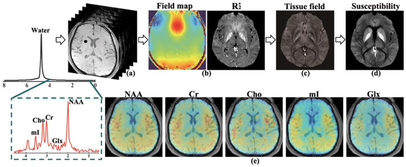
This work reports the feasibility of simultaneous QSM and high-resolution metabolite mapping from a single ¹H-MRSI scan using a new MRSI technique known as SPICE (SPectroscopic Imaging by exploiting spatiospectral CorrElation) (23,24). This capability is made possible by exploiting the fact that tissue susceptibility information is naturally encoded in the water spectroscopic signals from an MRSI scan if no water suppression is applied (Fig. 1). Conventional MRSI acquisitions usually apply several RF pulses to suppress the water and lipid signals, almost completely eliminating the susceptibility information. This problem is nicely overcome with SPICE which uses ultrashort-TE/short-TR acquisitions without water suppression (23,24). While SPICE has been used mainly for metabolic imaging, we extend its data acquisition and processing scheme to make it more suitable for simultaneous QSM and metabolic imaging. More specifically, in data acquisition we use dual-density sparse sampling and ramp sampling to extend k-space coverage to the level often required by QSM, while maintaining a reasonable SNR for the spatiospectral encodings used for metabolic imaging. In data processing, we take advantage of the larger number of echoes generated by the SPICE sequence (and any readily available anatomical priors) to produce high-quality QSM; we use a union-of-subspaces model to reconstruct the metabolite spatiospectral distributions. These features together allow us to obtain tissue susceptibility maps of the brain at a voxel size of 1.8×1.8×2.4 mm³ (or slightly smaller if the effect of the anatomical constraints is also taken into account), and metabolite maps at a nominal voxel size of 2.4×2.4×2.4 mm³ from a single 7-min scan. A more detailed description of our acquisition and processing schemes is given subsequently, which is followed by some representative experimental results to demonstrate the performance of the proposed method.

Figure 1.

Illustration of the proposed approach for simultaneous QSM and metabolic imaging using ¹H-MRSI signals acquired without water suppression.

METHODS

Data Acquisition

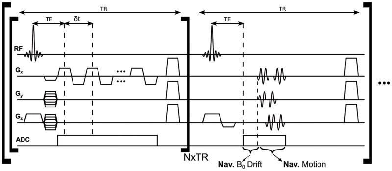
The proposed data acquisition scheme retains the main features of the FID-based SPICE sequence illustrated in Fig. 2. First, it uses ultrashort-TE/short-TR (3 ms/210 ms) acquisitions without water and lipid suppression pulses. Second, EPSI readout is used for rapid spatiospectral encoding with bipolar acquisitions; the EPSI trajectories used here have larger k-space coverage and, for each k-space location, longer echo spacing and much fewer spectral encodings than conventional EPSI trajectories, which are enabled by the SPICE subspace imaging framework. Third, interleaved navigator signals are collected for detection and correction of field drifts and head motion. Fourth, ramp sampling is employed in the readout direction (denoted as k_x) to increase k-space coverage, while maintaining the desired echo spacing and spectral bandwidth (BW) for MRSI given the practical ADC and gradient limits. Fifth, a sparse sampling scheme is used to increase k-space coverage along the phase encoding directions (i.e., k_y, k_z). More specifically, a dual density sparse sampling scheme is used with a fully sampled region (denoted as Ω₁) around k-space center and an undersampled region (denoted as Ω₂) in outer k-space. These sampling strategies with the (k, t)-space trajectories further illustrated in Fig. S1 are aimed at achieving enough spatial resolution for QSM while maintaining a sufficient number of spatiospectral encodings (with a larger fully-sampled central k-space) to ensure SNR for metabolic imaging. In short, the proposed data acquisition scheme has two distinct features as compared to conventional QSM and MRSI data acquisitions: a) it uses ultrashort-TE/short-TR with no water and lipid suppression, larger k-space coverage, larger echo spacing, and fewer echoes (spectral encodings) compared with conventional EPSI acquisitions, and b) it has much a longer echo train (i.e., more encodings for susceptibility changes) but smaller k-space coverage as compared with conventional GRE-based multi-echo QSM acquisitions. Our preliminary implementation of these data acquisition features has enabled QSM at a nominal in-plane resolution of 1.8×1.8 mm² and a through-plane resolution of 2.4 mm, and metabolic imaging at a 2.4×2.4×2.4 mm³ nominal resolution in about 7 minutes. Further improvement of the data acquisition scheme and its implementation can result in better spatial resolutions and shorter data acquisition times.

Figure 2.

Pulse sequence for the proposed FID acquisitions with ultrashort-TE, short-TR, no water suppression, bipolar acquisition, and ramp sampling (navigators acquired at every N TRs for field drift and motion tracking).

Data Processing

The (k,t)-space measurements over Ω₁ and Ω₂ using the proposed data acquisition can be expressed as:

$$d_l\left(\mathbf{k},t_n\right)=\int s_l(\mathbf{r})\rho \left(\mathbf{r},f\right)e^{-i2\pi \mathrm{\Delta }f\left(\mathbf{r}\right)t_n}{e}^{-i2\pi \mathbf{k}·\mathbf{r}}{e}^{-i2\pi f{t}_n}\mathrm{d}f\mathrm{d}\mathbf{r}+{\eta }_l\left(\mathbf{k},t_n\right),n=1,2,\dots ,N_{\mathrm{E}}$$ [1]

where ρ(r, f) denotes the spatiospectral distribution of all the molecular components (e.g., water, lipids, metabolites, etc.), s₁(r) the sensitivity map of the l-th channel, {t_n} the echo times, N_E the total number of echoes (i.e., number of time points or spectral encodings for each k-space location), and Δf(r) the field inhomogeneity containing the susceptibility information. We use the vector r = (x,y,z) to denote the spatial coordinates and k = (k_x,k_y,k_z) to represent the sampled k-space locations. The measurement noise η_l(k,t_n) is assumed to be complex white Gaussian. There are three key data processing problems in deriving the susceptibility and metabolite maps from the measured data: 1) reconstruction of the spatiospectral/spatiotemporal function from the sparsely sampled (k,t)-space data, 2) estimation of the susceptibility maps from the reconstructed spectroscopic signals, and 3) reconstruction of the metabolite signals. We will briefly describe our current solutions to these problems in the subsequent sections.

Interpolation of Sparse (k,t)-Space Data

With our current data acquisition scheme, the MRSI data are measured over a set of (k, t)-space points, divided into two disjoint sets Ω₁ and Ω₂, one for the fully covered central k-space and the other for undersampled outer k-space respectively (see Fig. S1a), and the time axis was slightly undersampled (with respect to the proton spectral BW). Temporal undersampling is not an issue for QSM because it is dependent on the water signals only; for metabolic imaging, temporal undersampling is taken care of in SPICE by using a subspace model (25,26). So, we are not going to delve in the issue here. To address the issue of sparse sampling in k-space, we resort to multichannel sensitivity encoding. More specifically, we interpolate the (k, t)-space signals along the k_y and k_z axes (i.e., the phase encoding directions along which sparse sampling is used) using a hybrid GRAPPA/SENSE method that exploits the special sampling pattern used. More specifically, a set of GRAPPA kernels {H_n} are first determined from the k-space samples for k ∈ Ω₁ for the “early” echoes (e.g., echo times at t_n for n = 1,2,…,32; approximately 60 ms for an echo spacing of 1.78 ms). A simple sliding-window scheme is employed to make use of the data from adjacent echoes to improve the estimation of {H_n} (i.e., using d_l(k,t_n) for k ∈ Ω₁ and n = m − 2, m − 1, m, m + 1, m + 2 to estimate H_m). After the {H_n} are determined, GRAPPA interpolation is applied to generate the missing data in Ω₂ for n = 1,2,…,32;. These interpolated k-space data are then Fourier reconstructed for each echo time t_n and each receiver channel. These reconstructions are then processed using an SVD-based scheme to extract the coil sensitivity maps s_l(r), assuming that s_l(r) is independent of the echo time t_n (27). After the s_l(r) are known, SENSE reconstruction is applied to the original undersampled data (d_l(k,t_n) for n = 1,2,…,N_E). Since the SENSE reconstructions with spatial regularization may not be data-consistent. we re-enforce data consistency by using the SENSE reconstructions and the coil sensitivity maps s_l(r) to generate the missing data in Ω₂ so that k-space is covered at the Nyquist rate with both measured and generated data for each time point. This hybrid GRAPPA/SENSE interpolation scheme seems to work better than GRAPPA interpolation especially for the late noisy echoes. However, a full analysis of its performance is needed, which is beyond the scope of the current paper.

Quantitative Susceptibility Mapping

The interpolated SPICE (k,t)-space data can be Fourier transformed for each echo time to give a sequence of images from which quantitative susceptibility information can be extracted. For clarity, we call them SPICE images and the method to derive the QSM from them SPICY-QSM. Note that the SPICE data contain signals from water, lipids, and metabolites but the metabolite signals are negligible as far as QSM is concerned, because the unsuppressed water and lipid signals are 3 to 4 orders of magnitude stronger. Therefore, for QSM calculations, we express the SPICE images as

$$\rho \left(\mathbf{r},t_n\right)=\left[{\rho }_{\mathrm{w}}\left(\mathbf{r}\right)+{\rho }_{\mathrm{f}}\left(\mathbf{r}\right){\varphi }_{\mathrm{f}}\left(\mathbf{r},t_n\right)\right]e^{-t_n/T_2^{\ast }(\mathbf{r})}{e}^{-i2\pi \mathrm{\Delta }f\left(\mathbf{r}\right)t_n},n=1,2,\dots ,N_{\mathrm{E}}$$ [2]

where ρ_w(r) and ρ_f(r) denote the proton density of water and lipids (with T₁ weighting) respectively, ${\varphi }_{\mathrm{f}}\left(\mathbf{r},t_n\right)={\displaystyle \sum _j}{\alpha }_j\left(\mathbf{r}\right)e^{i2\pi f_j{t}_n}$ the pre-determined spectral structures for lipids (with α_j being relative amplitudes of the lipid peaks), $T_2^{\ast }(\mathbf{r})$ the transverse relaxation times, and Δf(r) the total frequency offsets due to both the background field inhomogeneity f₀(r) and the tissue susceptibility induced field inhomogeneity f_s(r). Note that for demonstrating the feasibility of the proposed joint QSM and metabolite mapping technique, healthy subjects were scanned in this work, thus the lipid component was ignored for the signal model within the brain. Many methods have been proposed for estimating Δf(r), extracting f_s(r) from Δf(r), and solving the field-to-susceptibility inverse problem (28, 3); We build on these methods and take into account our specific data acquisition features to improve the estimation of the susceptibility map, denoted as χ(r) as described below.

First, to take advantage of the large number of echoes available in SPICE (90 ~ 100 vs. 6 ~ 8 in conventional QSM), we estimate Δf(r) by directly fitting the SPICE images to the complex exponential model in Eq. [2] using a nonlinear least-squares formulation (29). This scheme is optimal in the maximum likelihood sense for Gaussian noise and, perhaps even more importantly, it eliminates the need for phase unwrapping used in the conventional linear phase fitting schemes (which can be a difficult problem for low SNR data). Second, SPICE has a relatively smaller k-space coverage than conventional QSM methods. To improve spatial resolution for the susceptibility map beyond the k-space coverage, we constrain the susceptibility estimation using high-resolution anatomical constraints (3). These constraints can be obtained from the high-resolution anatomical scans typically acquired in standard neuroimaging protocols (e.g., MPRAGE scans). More specifically, we solve the following regularized dipole inversion (3):

$$\widehat{\mathbf{\chi }}=arg\underset{\mathbf{\chi }}{min}{\Vert {\mathbf{M}}_{\text{hr}}\mathbf{G}\mathbf{\chi }\Vert }_{1}s.t.{\Vert \mathbf{W}\left(\mathbf{D}\mathbf{\chi }-{\mathbf{f}}_{\mathrm{s}}\right)\Vert }_2^2\le \epsilon$$ [3]

where M_hr contains edge weights obtained from a high-resolution anatomical image, G is the gradient operator, χ the vector representation of the desired tissue susceptibility and D the matrix operator for the physical dipole convolution model. W contains weighting coefficients used to account for noise variation in the tissue field f_s as is done in (3), and ε is proportional to the noise level. The associated optimization problem is solved using a fixed point algorithm (3).

The overall data processing scheme for SPICY-QSM is illustrated in Fig. 1. More specifically, after Δf (total field inhomogeneity) is determined (Fig. 1b), the background field (due to imperfect shimming and susceptibility sources outside the ROI such as air/tissue interface) is removed by solving a Laplacian boundary value problem (28), producing the tissue field f_s(r) (Fig. 1c). Finally, tissue susceptibility (Fig. 1d) is reconstructed by solving the problem in Eq. [3].

Reconstruction of the Metabolite Spatiospectral Functions

Determination of the metabolite spatiospectral functions from the measured data can be done using the SPICE method for metabolic imaging (25,26). More specifically, we use a union-of-subspaces model to represent the spatiotemporal function ρ(r,t) in Eq. [1] as:

$$\begin{gathered} \rho \left(\mathbf{r},t\right)={\rho }_{\mathrm{m}}\left(\mathbf{r},t\right)+{\rho }_{\mathrm{w}}\left(\mathbf{r},t\right)+{\rho }_{\mathrm{f}}\left(\mathbf{r},t\right)+{\rho }_{\text{MM}}\left(\mathbf{r},t\right) \\ =\sum _{p_{\mathrm{m}}=1}^{R_{\mathrm{m}}}{u}_{p_{\mathrm{m}}}\left(\mathbf{r}\right)v_{p_{\mathrm{m}}}\left(t\right)+\sum _{p_{\mathrm{w}}=1}^{R_{\mathrm{w}}}{u}_{p_{\mathrm{w}}}\left(\mathbf{r}\right)v_{p_{\mathrm{w}}}\left(t\right)+\sum _{p_{\mathrm{f}}=1}^{R_{\mathrm{f}}}{u}_{p_{\mathrm{f}}}\left(\mathbf{r}\right)v_{p_{\mathrm{f}}}\left(t\right)+\sum _{p_{\text{MM}}=1}^{R_{\text{MM}}}{u}_{p_{\text{MM}}}\left(\mathbf{r}\right)v_{p_{\text{MM}}}\left(t\right) \end{gathered}$$ [4]

where ρ_m(r,t), ρ_w(r,t), ρ_f(r,t), and ρ_MM(r,t) denote the signals of metabolites, water, lipids, and macromolecules, respectively. This model assumes that each of the signal components resides in a low-dimensional subspace spanned by the bases {v_p,(t)} with spatial coefficients {u_p,(r)}, where “*” denotes “m”, “MM”, “w”, “f”, respectively. The subspace model significantly reduces the degrees of freedom of the spatiotemporal function. Separating the dominating water/lipid signals (after QSM) from the metabolite signals is done using a method similar to the one in Ref. (30). After water/lipid removal, the metabolite signals are reconstructed from the noisy residuals by solving the following optimization problem:

$$\left\{{\widehat{\mathbf{U}}}_{\mathrm{m}},{\widehat{\mathbf{U}}}_{\text{MM}}\right\}=arg\underset{{\mathbf{U}}_{\mathrm{m}},{\mathbf{U}}_{\text{MM}}}{min}{\Vert {\mathbf{d}}_{\text{rm}}-\mathbf{\Omega }\left\{\mathbf{FB}\odot \left({\mathbf{U}}_{\mathrm{m}}{\mathbf{V}}_{\mathrm{m}}+{\mathbf{U}}_{\text{MM}}{\mathbf{V}}_{\text{MM}}\right)\right\}\Vert }_2^2+{\lambda }_1{\mathrm{\Psi }}_1\left({\mathbf{U}}_{\mathrm{m}}\right)+{\lambda }_2{\mathrm{\Psi }}_2\left({\mathbf{U}}_{\text{MM}}\right)$$ [5]

where d_m is a vector containing the nuisance-removed (k,t)-space data, Ω is the sampling operator, F is the Fourier encoding operator, and B models the field inhomogeneity related phase terms (estimated from the companion water signals as described in QSM estimation). V_m and V_MM are matrix representations of the metabolite and macromolecule bases, both predetermined from training data (25,26). Ψ₁ and Ψ₂ are regularization functionals for metabolite and macromolecule components, respectively. In this work, Ψ₁ imposes edge-weighted spatial regularization and Ψ₂ is simply an l₂ penalty to improve conditioning. Solution of the problem in Eq. [5] has been discussed in (26).

In Vivo Experiments

Proton MRSI data without water suppression were collected using the SPICE sequence (Fig. 2) from healthy volunteers on a 3T Siemens scanner with IRB approval using a 20-channel head-neck coil. Two outer volume suppression bands (head to foot direction) were used to eliminate signal contamination from voxels outside the imaging volume. Other data acquisition parameters are: TR=210 ms, TE=3 ms, flip angle=31°, # of spectral encodings=92, echo spacing=1.78 ms, BW=167 kHz, FOV=230×230×72 mm³, and matrix size=124×128×30 (k_x, k_y, k_z). The center k_y×k_z (36×30) space was fully sampled while the outer region along k_y is undersampled by a factor of 2, thus leading to a 7-min scan (corresponding to an “effective” acceleration factor of 1.9 with elliptical sampling). Ramp sampling enabled a 13% resolution gain along the frequency encoding direction. To validate the susceptibility values generated from the proposed method, a corresponding 3D multi-echo GRE acquisition with flow compensation in both the slice and readout directions was performed over the same volume and FOV with a matrix size of 256×256×30 (spatial resolution=0.9×0.9×2.4 mm³, flip angle=20°, TR=50 ms, TE=4.55 ms, echo spacing=3.65 ms, # of echoes=8, BW/pixel=700 Hz). The same outer volume saturation bands were used for consistency. The Laplacian boundary method (28) and MEDI (3) were used to generate the QSM maps from the GRE data.

To compare the QSM results from both the SPICE and GRE datasets, anatomical images obtained from our experiments were registered using an affine transformation with 12 degrees of freedom in FSL (31). The coordinate transformation parameters were then used to align the susceptibility maps estimated from both datasets. To ensure similar regularization effects on solving the field-to-susceptibility inverse problem, the images from both the SPICE and GRE data were scaled to have the same noise level so that an identical regularization parameter can be used.

RESULTS

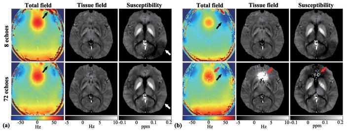
Figure 3 shows a set of representative QSM results from in vivo data. The effects of the number of echoes for the proposed processing method are also shown, in comparison with the results produced by the conventional QSM processing method (i.e., phase unwrapping followed by linear phase fitting). As can be seen, the field maps estimated using complex exponential fitting improve as the number of echoes increases (see the areas highlighted by arrows). Note also that the linear phase method yielded some “bad” fitting points (red arrows in Fig. 3) in regions with large field inhomogeneity, especially when a large number of echoes was used (due to unreliable phase unwrapping for noisy data of long echo times). The errors at these locations were carried over to the subsequently estimated tissue fields and susceptibility maps. Furthermore, with more echoes, ringing artifacts caused by low spatial resolution were reduced in the tissue field and susceptibility maps due to the physical constraints from the complex signal model and the dipole model. An improvement in SNR and a clearer delineation of the gray matter and white matter can also be observed with more echoes (highlighted by the white arrows in the left panel of Fig. 3).

Figure 3.

Total field inhomogeneity (left), tissue field (middle), and susceptibility maps (right) obtained from SPICE data with 8 and 72 echoes using: (a) complex exponential fitting without phase unwrapping, and (b) standard linear fitting with phase unwrapping. The estimated susceptibility maps from more echoes show improved SNR, reduced ringing artifacts and clearer delineation of gray matter and white matter (highlighted by white arrows), for the complex exponential fitting method. The linear fitting method yielded poor fitting in regions of large field inhomogeneity (highlighted by red arrows) when a large number of echoes were used.

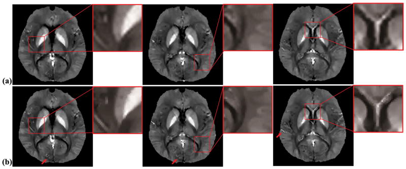
The effects of using high-resolution anatomical information to constrain the dipole inversion is demonstrated in Fig. 4. As can be seen from the susceptibility maps from the SPICE data produced using edge information from the SPICE data itself (Fig. 4a) and using edge information from high-resolution MPRAGE images (Fig. 4b), improved delineation of subcortical GM regions (e.g., the transition between Globus Pallidus and Putamen, boundaries between the caudate heads and the ventricles) and better definition of finer structures (as indicated by red arrows) can be observed.

Figure 4.

Tissue susceptibility estimated from the SPICE data for three consecutive slices using dipole inversion with (a) edge weights derived from the magnitude images of the MRSI data itself, and (b) edge weights derived from a high-resolution anatomical MPRAGE scan. Improved delineation of the subcortical GM regions and finer structures (indicated by red arrows) can be observed in the susceptibility maps generated by the proposed scheme (b).

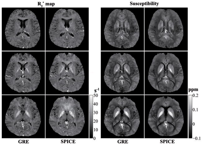
Figure 5 shows a set of representative $R_2^{\ast }$ and susceptibility maps for three slices obtained from both the GRE and SPICE data. The anatomical images (not shown here) from the two scans exhibit slightly different T₁ contrast due to the different TRs and flip angles used. The $R_2^{\ast }$ and susceptibility maps show very similar iron-content dependent tissue contrast. Although the GRE data have higher spatial resolution, the $R_2^{\ast }$ and susceptibility maps produced by the proposed method show better SNR (especially for the $R_2^{\ast }$ map), due to the larger number of echoes collected and the lower resolution. Note the susceptibility maps from both the GRE and SPICE scans are able to clearly resolve the major subcortical structures, e.g., Globus Pallidus (GP), Caudate Nucleus (CN), Putamen (PU). Mean susceptibility values for several representative subcortical GM regions are summarized in Table S1 (in the Supporting Material). These values are consistent with those reported in the literatures (32–34).

Figure 5.

$R_2^{\ast }$ and susceptibility maps obtained from the GRE and SPICE data for three representative slices. The results from both datasets clearly delineate iron rich subcortical GM regions including Globus Pallidus, Caudate Nucleus and Putamen. The results from the SPICE data have higher SNR (especially for the $R_2^{\ast }$ maps), due to a combination of more echoes and lower resolution.

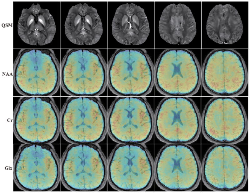
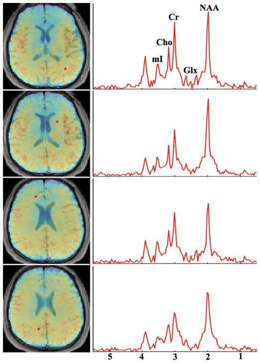
The susceptibility and metabolite maps, e.g., NAA, Creatine (Cr), and Glutamate + Glutamine (Glx) at five different slices across the 3D volume, obtained from a 7-min SPICE scan, are shown in Fig. 6. Spatially-resolved metabolite spectra with a spectral resolution of 0.038 ppm (or 4.68 Hz at 3T) from four representative voxels are shown in Fig. 7. The SNRs defined as the ratio between the spectral peaks and the noise standard deviation in the frequency domain for the NAA components at these voxels are 78.1, 78.4, 61.0 and 63.6 respectively. As can be seen, high-SNR metabolite spatiospectral distributions can be produced. Another set of representative experimental results from a different subject illustrating this capability is included in the Supporting Information (Fig. S2). Note again that both the QSM and metabolite information is obtained from a single ¹H-MRSI scan, as opposed to two separate long scans in the current practice. Further validation of this unprecedented capability will be reported in forthcoming papers.

Figure 6.

Quantitative susceptibility and metabolite maps for five representative slices across the brain obtained from a single 7-min SPICE acquisition. From top to bottom they are: susceptibility maps, NAA, Cr, and Glx maps, respectively. The metabolite maps are normalized individually and shown in color overlaid on the anatomical images.

Figure 7.

Localized spectra from four representative voxels (marked by red dots on the NAA maps on the left) obtained from the same data used to generate Fig. 6. The spectral SNR of the NAA peaks are 78.1, 78.4, 61.0 and 63.6 respectively. Note that the spectral resolution is determined by the spectral subspace other than the echo spacing in SPICE data.

DISCUSSION

This paper demonstrates the feasibility of SPICE for simultaneous mapping of brain tissue susceptibility (directly related to iron deposition (35)) and metabolites using a single ¹H-MRSI scan. The $R_2^{\ast }$ map, another useful biomarker for iron deposition in the brain (7), can also be derived from the proposed data acquisition as shown in Fig. 5. The unique data acquisition features of SPICE (i.e.., long echo train for metabolite mapping) were exploited for QSM (e.g., eliminating the need for phase unwrapping used in conventional QSM methods). While fully analyzing the effect of the number of echoes used for susceptibility estimation is beyond the scope of the current paper, a simulation study was performed to confirm our observation. Specifically, a set of parameter maps including ρ₀(r), $T_2^{\ast }\left(\mathbf{r}\right)$, Δf₀(r), and χ(r) were first estimated from a high-resolution GRE dataset, and used to synthesize a 92-echo image series (for the same echo times used as in the SPICE acquisition) using the physical dipole convolution model (f_s = Dχ) and the signal model in Eq. [2]. Complex Gaussian noise (with standard deviation being 1% the mean proton density value) was added to the image series to mimic a similar noise level encountered in practical GRE acquisitions. Figure S3 (in the Supporting Information) shows the tissue field and corresponding relative errors generated by the proposed processing using different numbers of echoes. As can be seen, more echoes helped reduce the errors in the estimated tissue field significantly, thus reducing the potential error propagation from the estimated tissue field to the final susceptibility reconstruction. Moreover, the acquisition of many echoes is also expected to be beneficial when complex signal models are used to account for nonlinear phase variations such as those described in Refs. (36, 37).

In order to generate a sufficient number of spectral encodings for metabolite mapping, the SPICE acquisition uses longer TR than standard QSM thus covers a smaller region of k-space given the same acquisition time. This issue was addressed in this work by a combination of the dipole convolution physical model and the use of morphological information from high-resolution anatomical images (e.g., MPRAGE scan). This allowed us to improve the spatial resolution beyond what was offered by the nominal k-space coverage (~1.8×1.8×2.4 mm³) of our SPICE data. Our preliminary results show a clear delineation of iron-rich subcortical GM structures (e.g., GP, CN, and PU) that possess super-intensive bulk susceptibility, which are consistent with the existing QSM data (25,26). It is worth noting that our acquisition can also achieve higher resolution for QSM at the expense of longer acquisition time. To illustrate this, a 15-min in vivo experiment with spatial resolution of 1.8×1×1 mm³ was performed. In this scan, the sampling for the original k-space coverage (1.8×1.8×2.4 mm³ voxel size) remained the same while the outer k-space was further undersampled by a factor of 3 along k_y and a factor of 2 along k_z. The QSM maps and the metabolite maps from this data were shown in the Supporting Information (Fig. S4). As can be seen, QSM with comparable resolution to standard QSM can be obtained, along with simultaneously obtained metabolite maps. Note that due to the multiple nonlinear processing steps involved, a full characterization of the SNR and resolution of the final QSM maps is challenging. This issue will be addressed in a subsequent paper.

Several aspects of the proposed acquisition and processing methods can be further improved. For example, we can better integrate parallel imaging into our data acquisition and processing schemes to enhance resolution and/or data acquisition speed. For example, a better sparse sampling pattern design for the outer k-space region combined with more advanced reconstruction methods can enable larger acceleration factors. Methods taking advantage of the sparse and low-rank structures present in the desired spatiotemporal distributions can be explored to improve the reconstruction of the SPICE images used for QSM processing. The coil sensitivities are currently estimated from the EPSI data itself in this work. However, the proposed method does not prevent the use of sensitivity determined from auxiliary high-resolution anatomical scans as long as data registration is properly done.

Our current method uses the MPRAGE data to extract the edge weights used in solving the problem in Eq. [3]. Other high resolution scans or even a pre-determined high-resolution atlas with different contrast (such as T₂* weighting) can also be used. Furthermore, enforcing the edge prior through the weighted L₁ regularization has been shown to tolerate edge mismatch between anatomical images and susceptibility maps (3). Sparsity-promoting regularizations other than weighted L₁ or L₂ can also be used (38). The intra-volume flow has been shown to have an effect on the QSM results. Flow-compensation using first-order moment nulling gradients, as described in Ref. (37), can be included into the SPICE acquisition to address this issue, i.e., before the spatiospectral encoding echo trains and during the even echoes. This would lead to slightly longer echo times and reduce the number of echoes available for spatiospectral reconstruction. These tradeoffs should be considered in practical application context.

CONCLUSIONS

This paper demonstrates the feasibility of simultaneous QSM and metabolic imaging of the brain using SPICE. The proposed data acquisition scheme is built on the SPICE sequence, integrating ultrashort-TE/short-TR acquisitions with no water suppression and sparse sampling. The proposed processing scheme uses model-based processing to obtain both the susceptibility and metabolite maps. This new imaging capability, when fully developed, may prove useful for a wide range of applications including the study of brain metabolism and neurodegenerative diseases.

Supplementary Material

Supp figure&tables

Table S1. Mean susceptibility values in parts per billion (ppb) for three different subcortical GM regions.

Figure S1. The proposed (a) sampling trajectories in the phase encoding directions (k_y, k_z); and (b) EPSI readouts used in SPICE (red) in comparison to the standard EPSI in conventional MRSI methods.

Figure S2. Another set of experimental results from a single 5-min ¹H-MRSI scan (nominal voxel size: 2.1×2.4×3 mm³).

Figure S3. Effect of the echo train length on the tissue field estimation (numerical simulation): (a) estimated tissue field and error maps using different numbers of echoes, and (b) corresponding relative l₂ errors for the different cases in (a).

Figure S4. Results from a 15-min in vivo experiment producing QSM with a spatial resolution of 1.8×1×1 mm³ and MRSI with a resolution of 2.4×2.4×2.4 mm³.

References

- 1.Wang Y, Liu T. Quantitative susceptibility mapping (QSM): decoding MRI data for a tissue magnetic biomarker. Magn Reson Med. 2015;73:82–101. doi: 10.1002/mrm.25358. [DOI] [PMC free article] [PubMed] [Google Scholar]
- 2.Liu T, Wisnieff C, Lou M, Chen W, Spincemaille P, Wang Y. Nonlinear formulation of the magnetic field to source relationship for robust quantitative susceptibility mapping. Magn Reson Med. 2013;69:467–476. doi: 10.1002/mrm.24272. [DOI] [PubMed] [Google Scholar]
- 3.Liu J, Liu T, de Rochefort L, Ledoux J, Khalidov I, Chen W, Tsiouris AJ, Wisnieff C, Spincemaille P, Prince MR, Wang Y. Morphology enabled dipole inversion for quantitative susceptibility mapping using structural consistency between the magnitude image and the susceptibility map. NeuroImage. 2012;59:2560–2568. doi: 10.1016/j.neuroimage.2011.08.082. [DOI] [PMC free article] [PubMed] [Google Scholar]
- 4.Xu B, Liu T, Spincemaille P, Prince M, Wang Y. Flow compensated quantitative susceptibility mapping for venous oxygenation imaging. Magn Reson Med. 2014;72:438–445. doi: 10.1002/mrm.24937. [DOI] [PMC free article] [PubMed] [Google Scholar]
- 5.Haacke EM, Tang J, Neelavalli J, Cheng YCN. Susceptibility mapping as a means to visualize veins and quantify oxygen saturation. J Magn Reson Imaging. 2010;32:663–676. doi: 10.1002/jmri.22276. [DOI] [PMC free article] [PubMed] [Google Scholar]
- 6.Fan AP, Bilgic B, Gagnon L, Witzel T, Bhat H, Rosen BR, Adalsteinsson E. Quantitative oxygenation venography from MRI phase. Magn Reson Med. 2014;72:149–159. doi: 10.1002/mrm.24918. [DOI] [PMC free article] [PubMed] [Google Scholar]
- 7.Barbosa JH, Santos AC, Tumas V, Liu M, Zheng W, Haacke EM, Salmon CE. Quantifying brain iron deposition in patients with Parkinson’s disease using quantitative susceptibility mapping, R2 and . Magn Reson Imaging. 2015;33:559–565. doi: 10.1016/j.mri.2015.02.021. [DOI] [PubMed] [Google Scholar]
- 8.de Graaf RA. In Vivo NMR Spectroscopy: Principles and Techniques. 2. John Wiley & Sons, Ltd; 2007. [Google Scholar]
- 9.Davison JE, Davies NP, Wilson M, Sun Y, Chakrapani A, McKiernan PJ, Walter JH, Gissen P, Peet AC. MR spectroscopy-based brain metabolite profiling in propionic acidaemia: metabolic changes in the basal ganglia during acute decompensation and effect of liver transplantation. Orphanet J Rare Dis. 2011;6:19. doi: 10.1186/1750-1172-6-19. [DOI] [PMC free article] [PubMed] [Google Scholar]
- 10.Oz G, Alger JR, Barker PB, et al. Clinical proton MR spectroscopy in central nervous system disorders. Radiology. 2014;270:658–679. doi: 10.1148/radiol.13130531. [DOI] [PMC free article] [PubMed] [Google Scholar]
- 11.Wilson M, Cummins CL, Macpherson L, Sun Y. Magnetic resonance spectroscopy metabolite profiles predict survival in pediatric brain tumors. Eur J Cancer. 2013;49:457–464. doi: 10.1016/j.ejca.2012.09.002. [DOI] [PMC free article] [PubMed] [Google Scholar]
- 12.Preul MC, Caramanos Z, Collins DL, Villemure JG, Leblanc R, Olivier A, Pokrupa R, Arnold DL. Accurate, noninvasive diagnosis of human brain tumors by using proton magnetic resonance spectroscopy. Nat Med. 1996;2:323–325. doi: 10.1038/nm0396-323. [DOI] [PubMed] [Google Scholar]
- 13.Astrakas LG, Zurakowski D, Tzika AA, Zarifi MK, Anthony DC, DeGirolami U, Tarbell NJ, Black PM. Noninvasive magnetic resonance spectroscopic imaging biomarkers to predict the clinical grade of pediatric brain tumors to predict the clinical grade of pediatric brain tumors. Clin Cancer Res. 2004;10:8220–8228. doi: 10.1158/1078-0432.CCR-04-0603. [DOI] [PubMed] [Google Scholar]
- 14.Sorensen AG. Magnetic resonance as a cancer imaging biomarker. J Clin Oncol. 2006;24:3274–3281. doi: 10.1200/JCO.2006.06.6597. [DOI] [PubMed] [Google Scholar]
- 15.Acosta-Cabronero J, Williams GB, Cardenas-Blanco A, Arnold RJ, Lupson V, Nestor PJ. In vivo quantitative susceptibility mapping (QSM) in Alzheimer’s disease. PLoS One. 2013;8:e81093. doi: 10.1371/journal.pone.0081093. [DOI] [PMC free article] [PubMed] [Google Scholar]
- 16.Colla M, Ende G, Bohrer M, Deuschle M, Kronenberg G, Henn F, Heuser I. MR spectroscopy in Alzheimer’s disease: gender differences in probabilistic learning capacity. Neurobiol Aging. 2003;24:545–552. doi: 10.1016/s0197-4580(02)00189-6. [DOI] [PubMed] [Google Scholar]
- 17.Langkammer C, Liu T, Khalil M, Enzinger C, Jehna M, Fuchs S, Fazekas F, Wang Y, Ropele S. Quantitative susceptibility mapping in multiple sclerosis. Radiology. 2013;267:551–559. doi: 10.1148/radiol.12120707. [DOI] [PMC free article] [PubMed] [Google Scholar]
- 18.Lotfipour AK, Wharton S, Schwarz ST, Gontu V, Schäfer A, Peters AM, Bowtell RW, Auer DP, Gowland PA, Bajaj NPS. High resolution magnetic susceptibility mapping of the substantia nigra in Parkinson’s disease. J Magn Reson Imaging. 2012;35:48–55. doi: 10.1002/jmri.22752. [DOI] [PubMed] [Google Scholar]
- 19.Nelsona SJ. Assessment of therapeutic response and treatment planning for brain tumors using metabolic and physiological MRI. NMR Biomed. 2011;24:734–749. doi: 10.1002/nbm.1669. [DOI] [PMC free article] [PubMed] [Google Scholar]
- 20.Brown TR, Kincaid BM, Ugurbil K. NMR chemical shift imaging in three dimensions. Proc Natl Acad Sci USA. 1982;79:3523–3526. doi: 10.1073/pnas.79.11.3523. [DOI] [PMC free article] [PubMed] [Google Scholar]
- 21.Langkammer C, Bredies K, Poser BA, Barth M, Reishofer G, Fan AP, Bilgic B, Fazekas F, Mainero C, Ropele S. Fast quantitative susceptibility mapping using 3D EPI and total generalized variation. Neuroimage. 2015;111:622–30. doi: 10.1016/j.neuroimage.2015.02.041. [DOI] [PubMed] [Google Scholar]
- 22.Cao P, Wu EX. Accelerating phase-encoded proton MR spectroscopic imaging by compressed sensing. J Magn Reson Imaging. 2015;41:487–495. doi: 10.1002/jmri.24553. [DOI] [PubMed] [Google Scholar]
- 23.Sheikh M, Lam F, Ma C, Clifford B, Liang Z-P. Rapid, high-resolution 3D 1H-MRSI of the brain based on FID acquisitions. ISMRM. 2016:2353. [Google Scholar]
- 24.Lam F, Li Y, Clifford B, Peng X, Liang Z-P. Simultaneous mapping of brain metabolites, macromolecules and tissue susceptibility using SPICE. ISMRM. 2017:1249. [Google Scholar]
- 25.Lam F, Liang Z-P. A subspace approach to high-resolution spectroscopic imaging. Magn Reson Med. 2014;71:1349–1357. doi: 10.1002/mrm.25168. [DOI] [PMC free article] [PubMed] [Google Scholar]
- 26.Lam F, Ma C, Clifford B, Johnson CL, Liang Z-P. High-resolution 1H-MRSI of the brain using SPICE: Data acquisition and image reconstruction. Magn Reson Med. 2015;76:1059–1070. doi: 10.1002/mrm.26019. [DOI] [PMC free article] [PubMed] [Google Scholar]
- 27.Bydder M, Hamilton G, Yokoo T, Sirlin CB. Optimal phased-array combination for spectroscopy. Magn Reson Imaging. 2008;26:847–850. doi: 10.1016/j.mri.2008.01.050. [DOI] [PMC free article] [PubMed] [Google Scholar]
- 28.Zhou D, Liu T, Spincemaille P, Wang Y. Background field removal by solving the Laplacian boundary value problem. NMR Biomed. 2014;27:312–319. doi: 10.1002/nbm.3064. [DOI] [PubMed] [Google Scholar]
- 29.Golub G, Pereyra V. Separable nonlinear least squares: the variable projection method and its applications. Inverse Problems. 2013;19:R1–R26. [Google Scholar]
- 30.Ma C, Lam F, Johnson CL, Liang Z-P. Removal of nuisance signals from limited and sparse 1H MRSI data using a union-of-subspaces model. Magn Reson Med. 2016;75:488–497. doi: 10.1002/mrm.25635. [DOI] [PMC free article] [PubMed] [Google Scholar]
- 31.Jenkinson M, Smith S. A global optimization method for robust affine registration of brain images. Med Image Anal. 2001;5:143–156. doi: 10.1016/s1361-8415(01)00036-6. [DOI] [PubMed] [Google Scholar]
- 32.Sun H, Wilman AH. Quantitative susceptibility mapping using single-shot echo-planar imaging. Magn Reson Med. 2015;73:1932–1938. doi: 10.1002/mrm.25316. [DOI] [PubMed] [Google Scholar]
- 33.Sun H, Seres P, Wilman AH. Structural and functional quantitative susceptibility mapping from standard fMRI studies. NMR Biomed. 2017 doi: 10.1002/nbm.3619. [DOI] [PubMed] [Google Scholar]
- 34.Lin PY, Chao TC, Wu ML. Quantitative susceptibility mapping of human brain at 3T: a multisite reproducibility study. Am J Neuroradiol. 2015;36:467–474. doi: 10.3174/ajnr.A4137. [DOI] [PMC free article] [PubMed] [Google Scholar]
- 35.Langkammer C, Schweser F, Krebs N, Deistung A, Goessler W, Scheurer E, Sommer K, Reishofer G, Yen K, Fazekas F, Ropele S, Reichenbach JR. Quantitative susceptibility mapping (QSM) as a means to measure brain iron? A post mortem validation study. NeuroImage. 2012;62:1593–1599. doi: 10.1016/j.neuroimage.2012.05.049. [DOI] [PMC free article] [PubMed] [Google Scholar]
- 36.Dimov AV, Liu T, Spincemaille P, Ecanow JS, Tan H, Edelman RR, Wang Y. Joint estimation of chemical shift and quantitative susceptibility mapping (Chemical QSM) Magn Reson Med. 2015;73:2100–2110. doi: 10.1002/mrm.25328. [DOI] [PMC free article] [PubMed] [Google Scholar]
- 37.Xu B, Liu T, Spincemaille P, Prince M, Wang Y. Flow compensated quantitative susceptibility mapping for venous oxygenation imaging. Magn Reson Med. 2014;72:438–445. doi: 10.1002/mrm.24937. [DOI] [PMC free article] [PubMed] [Google Scholar]
- 38.Langkammer C, Schweser F, Shmueli K, Kames C, Li X, Guo L, Milovic C, Kim J, Wei H, Bredies K, Buch S, Guo Y, Liu Z, Meineke J, Rauscher A, Marques JP, Bilgic B. Quantitative susceptibility mapping: Report from the 2016 reconstruction challenge. Magn Reson Med. 2017 doi: 10.1002/mrm.26830. [DOI] [PMC free article] [PubMed] [Google Scholar]
Associated Data
This section collects any data citations, data availability statements, or supplementary materials included in this article.
Supplementary Materials