Optimizing Chemical Reactions with Deep Reinforcement Learning

Abstract

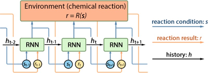
Deep reinforcement learning was employed to optimize chemical reactions. Our model iteratively records the results of a chemical reaction and chooses new experimental conditions to improve the reaction outcome. This model outperformed a state-of-the-art blackbox optimization algorithm by using 71% fewer steps on both simulations and real reactions. Furthermore, we introduced an efficient exploration strategy by drawing the reaction conditions from certain probability distributions, which resulted in an improvement on regret from 0.062 to 0.039 compared with a deterministic policy. Combining the efficient exploration policy with accelerated microdroplet reactions, optimal reaction conditions were determined in 30 min for the four reactions considered, and a better understanding of the factors that control microdroplet reactions was reached. Moreover, our model showed a better performance after training on reactions with similar or even dissimilar underlying mechanisms, which demonstrates its learning ability.

Short abstract

Chemical reactions were optimized through deep reinforcement learning. By iteratively analyzing reaction results and choosing new conditions for improvement, optimal conditions were found in 30 min.

Introduction

Unoptimized chemical reactions are costly and inefficient in regard to time and reagents. A common way for chemists to optimize reactions is to change a single experimental condition at a time while fixing all the others.¹ This approach will often miss the optimal conditions. Another way is to search exhaustively all combinations of reaction conditions via batch chemistry. Although this approach has a better chance to find the global optimal condition, it is time-consuming and expensive. An efficient and effective framework to optimize chemical reactions will be of great importance for both academic research and industrial production. We present here one potential approach to achieving this goal.

There have been various attempts to use automated algorithms to optimize chemical reactions.² Jensen and co-workers utilized the simplex method to optimize reactions in microreactors.^1,3 Poliakoff and co-workers constructed a system with what they called a stable noisy optimization by branch and fit (SNOBFIT) algorithm to optimize reactions in supercritical carbon dioxide.⁴ Jensen and co-workers optimized the Suzuki–Miyaura reaction, which involves discrete variables, by automated feedback.⁵ There are also numerous studies on optimizing a chemical reaction in flow reactors.⁶ Truchet and co-workers optimized the Heck–Matsuda reaction with a modified version of the Nelder–Mead method.⁷ Lapkin and co-workers developed a model-based design of experiments and self-optimization approach in flow.⁸ Ley and co-workers built a novel Internet-based system for reaction monitoring and optimization.⁹ Bourne and co-workers developed automated continuous reactors, which use high performance liquid chromatography (HPLC)¹⁰ or online mass spectrometry (MS)¹¹ for reaction monitoring and optimization. deMello and co-workers designed a microfluidic reactor for controlled synthesis of fluorescent nanoparticles.¹² Cronin and co-workers provided a flow-NMR platform for monitoring and optimizing chemical reactions.¹³ We are going to suggest a different approach that we believe will further improve the reaction optimization process.

Recently, the idea of machine learning and artificial intelligence^14,15 has produced surprising results in the field of theoretical and computational chemistry. Aspuru-Guzik and co-workers designed graph convolutional neural networks for molecules,¹⁶ and realized automatic chemical design with data-driven approaches.¹⁷⁻¹⁹ One step further, Pande and co-workers extended the idea of graph convolution,²⁰ and proposed one-shot learning for drug discovery.²¹ Meanwhile, both the Aspuru-Guzik group and the Jensen group derived intuition of predicting organic reactions from the machine learning perspective.^22,23 Besides, the machine learning approach also succeeded in using experimental data to make predictions. Norquist and co-workers predicted the reaction outcome from failed experiments with the help of a support vector machine.²⁴ Sebastian and co-workers utilized neural networks to identify skin cancers,²⁵ Zare and co-workers applied machine learning/statistics on mass spectrometry data to determine cancer states²⁶ and identify personal information.²⁷ Inspired by all the current successes achieved for prediction, we have applied the decision-making framework to problems in chemistry, specifically chemical reactions.

We developed a model we call the Deep Reaction Optimizer (DRO) to guide the interactive decision-making procedure in optimizing reactions by combining state-of-the-art deep reinforcement learning with the domain knowledge of chemistry. Iteratively, the DRO interacts with chemical reactions to obtain the current experimental condition and yield, and determines the next experimental condition to attempt. In this way, DRO not only served as an efficient and effective reaction optimizer but also provided us a better understanding of the mechanism of chemical reactions than that obtained using traditional approaches. With extensive experiments on simulated reactions, our method outperformed several state-of-the-art blackbox optimization algorithms of covariance matrix adaption–evolution strategy (CMA-ES),²⁸ the Nelder–Mead simplex method,²⁹ and stable noisy optimization by branch and fit (SNOBFIT)³⁰ by using 71% fewer steps. We also demonstrated that DRO applied to four real microdroplet reactions found the optimal experimental conditions within 30 min, owing its success to the acceleration of reaction rates in microdroplet chemistry^31,32 and to its efficient optimization algorithm. Moreover, our model achieved better performance after running on real reactions, showing its capability to learn from past experience.

Besides, our model showed strong generalizability in two ways: First, based on optimization of a large family of functions, our optimization goal can be not only yield but also selectivity, purity, or cost, because all of them can be modeled by a function of experimental parameters. Second, a wide range of reactions can be accelerated by 10³ to 10⁶ times in microdroplets.³³ Showing that a microdroplet reaction can be optimized in 30 min by our model of DRO, we therefore propose that a large class of reactions can be optimized by our model. The wide applicability of our model suggests it to be useful in both academic research and industrial production.

Method

Optimization of Chemical Reactions

A reaction can be viewed as a system taking multiple inputs (experimental conditions) and providing one desired output. Example inputs include temperature, solvent composition, pH, catalyst, and time. Example outputs include product yield, selectivity, purity, and cost. The reaction can be modeled by a function r = R(s), where s stands for the experimental conditions and r denotes the objective, say, the yield. The function R describes how the experimental conditions s affect r. Reaction optimization refers to the procedure for searching the combination of experimental conditions that achieves the objective in an optimal manner, also, desirably with the least number of steps.

In general, chemical reactions are expensive and time-consuming to conduct, and the outcome can vary largely, which is caused in part by measurement errors. Motivated by these considerations, we developed our model of Deep Reaction Optimizer (DRO) with the help of reinforcement learning.

Deep Reaction Optimizer by Reinforcement Learning

Reinforcement learning is an area of machine learning concerned with how the “decision-maker(s)” ought to take sequential “actions” in a prescribed “environment” so as to maximize a notion of cumulative “reward”. In the context of reaction optimization, where the reaction is the environment, an algorithm or person (decision-maker) decides what experimental conditions to try (actions), in order to achieve the highest yield (reward).

Mathematically, the underlying model for reinforcement learning is the Markov decision process characterized by , where

• denotes the set of states s. In the context of reaction optimization, is the set of all possible combinations of experimental conditions.

• denotes the set of actionsa. In the context of reaction optimization, is the set of all changes that can be made to the experimental conditions, for example, increasing the temperature by 10 °C and so forth.

• {P_sa} denotes the state transition probabilities. Concretely, P_sa specifies the probability of transiting from s to another state with action a. In the context of a chemical reaction, P_sa specifies to what experimental conditions the reaction will move if we decide to make a change a to the experimental condition s. Intuitively, P_sa measures the inaccuracy when operating the instrument. For example, the action of increasing the temperature by 10 °C may result in a temperature increase of 9.5–10.5 °C.

• R denotes the reward function of state s and action a. In the environment of a reaction, the reward r is only a function of state s, i.e., a certain experimental condition s (state) is mapped to yield r (reward) by the reward function r = R(s).

The core of reinforcement learning is to search for an optimal policy, which captures the mechanism of decision-making. In the context of chemical reactions, the policy refers to the algorithm that interacts with the chemical reaction to obtain the current reaction condition and reaction yield, from which the next experimental conditions are chosen. Rigorously, we define the policy as the function π, which maps from the current experimental condition s_t and history of the experiment record to the next experimental condition, that is,

1

where is the history, and t records the number of steps we have taken in reaction optimization.

Intuitively, the optimization procedure can be explained as follows: We iteratively conduct an experiment under a specific experimental condition and record the yield. Then the policy function makes use of all the history of experimental record (what condition led to what yield) and tells us what experimental condition we should try next. This procedure is described in Algorithm 1 and illustrated in Scheme 1.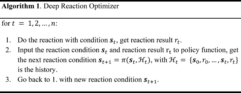

Scheme 1. Visualization of the DRO Model Unrolled over Three Time Steps.

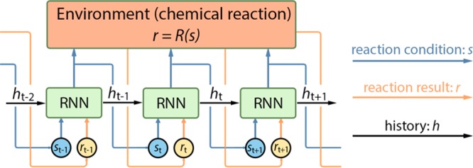
As stated earlier, the environment of chemical reaction is characterized by the reaction function of r = R(s).

Recurrent Neural Network as the Policy Function

Our DRO model employs the recurrent neural network (RNN) to fit the policy function π under the settings of chemical reactions. A recurrent neural network is a nonlinear neural network architecture in machine learning. An RNN parametrized by θ usually takes the form of

2

where x_t and x_t+1 are the data at time steps t and t + 1, and h_t and h_t+1 refer to the hidden state at time steps t and t + 1. The hidden state contains the history information that RNN passes to the next time step, enabling the network to remember past events, which can be used to interpret new inputs. This property makes RNN suitable as the policy for making decisions, which takes a similar form of the policy function of eq 1. A modified version of RNN to model the policy function,

3

where at time step t, h_t is the hidden state to model the history , s_t, denotes the state of reaction condition, and r_t is the yield (reward) of reaction outcome. The policy of RNN maps the inputs at time step t to outputs at time step t + 1. The model is exemplified as in Scheme 1.

Training the DRO

The objective in reinforcement learning is to maximize the reward by taking actions over time. Under the settings of reaction optimization, our goal is to find the optimal reaction condition with the least number of steps. Then, our loss function l(θ) for the RNN parameters θ is defined as

4

where T is the time horizon (total number of steps) and r_t is the reward at time step t. The term inside the parentheses measures the improvement we can achieve by iteratively conducting different experiments. The loss function (eq 4) encourages reaching the optimal condition faster, in order to address the problem that chemical reactions are expensive and time-consuming to conduct.

The loss function l(θ) is minimized with respect to the RNN parameters θ by an algorithm of gradient descent, which computes the gradient of the loss function ∇_θl(θ), and updates the parameter of θ by the rule θ ← θ – η∇_θl(θ), where η is the step size.

Results and Discussion

Pretraining on Simulated Reactions

As mentioned earlier, chemical reactions are time-consuming to evaluate. Although our DRO model can greatly accelerate the procedure, we still propose to first train the model on simulated reactions (a technique called pretraining in machine learning). A class of nonconvex “mixture Gaussian density functions” is used as the simulated reactions environment r = R(s). The nonconvex functions could have multiple local minima.

The motivation for using a mixture of Gaussian density functions comes from the idea that they can be used to approximate arbitrarily close all continuous functions on a bounded set. We assume that the response surface for most reactions is a continuous function, which can be well approximated by a mixture of Gaussian density functions. Besides, a mixture of Gaussian density functions often has multiple local minima. The rationale behind this is that the response surface of a chemical reaction may also have multiple local optima. As a result, we believe a mixture of Gaussian density functions can be a good class of function to simulate real reactions.

We compared our DRO model with several state-of-the-art blackbox optimization algorithms of covariance matrix adaption–evolution strategy (CMA-ES), Nelder–Mead simplex method, and stable noisy optimization by branch and fit (SNOBFIT) on another set of mixture Gaussian density functions that are unseen during training. This comparison is a classic approach for model evaluation in machine learning. We use “regret” to evaluate the performance of the models. The regret is defined as

5

and it measures the gap between the current reward and the largest reward that is possible. Lower regret indicates better optimization. In the context of simulated reaction, the functions are randomly generated and we can access the global maximum/minimum value of the function, which corresponds to the “largest reward that is possible”.

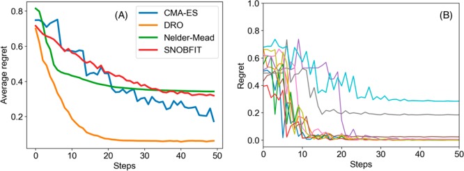
Figure 1A shows the average regret versus time steps of the two algorithms from which we see that DRO outperforms CMA-ES significantly by reaching a lower regret value in fewer steps. For 5000 random functions, DRO can reach the criterion of regret ≤0.05 in approximately 32 steps, on average, whereas CMA-ES needs 111 steps, SNOBFIT needs 187 steps, and Nelder–Mead fails to reach the criterion. Overall, the experiments demonstrate that our model outperforms those algorithms on the task of nonconvex function optimization, i.e., simulated chemical reaction optimization.

Figure 1.

(A) Comparison of average regret of CMA-ES, Nelder–Mead simplex method, SNOBFIT, and DRO. The average regret is calculated as the average regret on 1000 random nonconvex functions. (B) The observed regret of 10 random nonconvex functions in which each line is the regret of one function.

Randomized Policy for Deep Exploration

Although our model of DRO optimizes nonconvex functions faster than CMA-ES, we observe that DRO sometimes get stuck in a local maximum (Figure 1B) because of the deterministic “greedy” policy, where greedy means making the locally optimal choice at each stage without exploration. In the context of reaction optimization, a greedy policy will stick to one reaction condition if it is better than any other conditions observed. However, the greedy policy will get trapped in a local optimum, failing to explore some regions in the space of experimental conditions, which may contain a better reaction condition that we are looking for. To further accelerate the optimization procedure in this aspect, we proposed a randomized exploration regime to explore different experimental conditions, in which randomization means drawing the decision randomly from a certain probability distribution. This idea came from the work of Van Roy and co-workers,³⁴ which showed that deep exploration can be achieved from randomized value function estimates. The stochastic policy also addresses the problem of randomness in chemical reactions.

A stochastic recurrent neural network was used to model a randomized policy,³⁵ which can be written as

6

Similar to the notations introduced before, the RNN is used to generate the mean μ_t+1, and the covariance matrix Σ_t+1; the next state s_t+1 is then drawn from a multivariate Gaussian distribution of , at time step t + 1. This approach achieved deep exploration in a computationally efficient way.

Figure 2 compares between the greedy policy and the randomized policy on another group of simulated reactions. Although the randomized policy was slightly slower, it arrives to a better function value owing to its more efficient exploration strategy. Comparing the randomized policy with a deterministic one, the average regret was improved from 0.062 to 0.039, which shows a better chance of finding the global optimal conditions.

Figure 2.

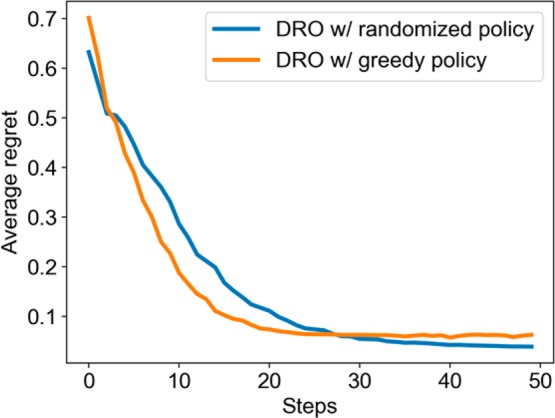
Comparison of deterministic policy and randomized policy in the model of DRO.

Optimization of Real Reactions

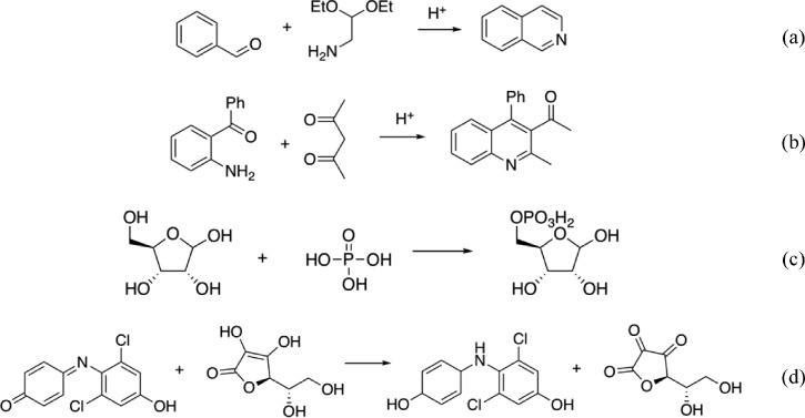
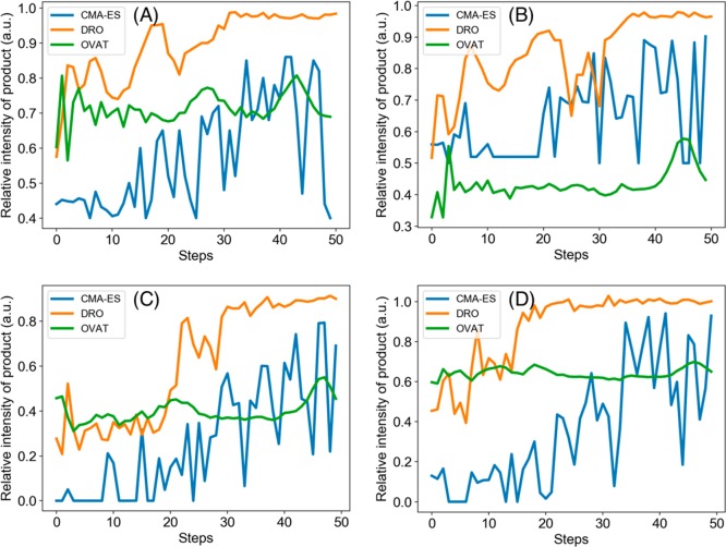
We carried out four experiments in microdroplets and recorded the production yield: The Pomeranz–Fritsch synthesis of isoquinoline (Scheme 2a),³⁶ Friedländer synthesis of a substituted quinoline (Scheme 2b),³⁶ the synthesis of ribose phosphate (Scheme 2c),³⁷ and the reaction between 2,6-dichlorophenolindophenol (DCIP) and ascorbic acid (Scheme 2d).³⁸ In all four reactions, two reagents are filled in separate syringes. Solutions from those two syringes are mixed in a T-junction and sprayed from an electrospray ionization (ESI) source with high voltage and pressure. The flow rate (from 0 to 10 μL/min), voltage (from 0 to 10 kV), and pressure (from 0 to 120 psi) applied on the spray source are the experimental parameters that are optimized, with all other conditions held constant. In these four reactions, the variables are continuous. The reaction yield of product, which was measured by mass spectrometry, was set as the optimization objective. The initial reaction conditions are randomly chosen. DRO, CMA-ES, and one variable at a time (OVAT) methods were compared on the four reactions. The DRO model had been pretrained on simulated reaction data, and the “OVAT” refers to the method of scanning a single experimental condition while fixing all the others, i.e., hold all variables but one, and see the best result when the one free variable is varied. As mentioned before, CMA-ES is the state-of-the-art blackbox optimizer in machine learning and OVAT is the classic approach followed by many researchers and practitioners in chemistry. DRO outperformed the other two methods by reaching a higher yield in fewer steps (Figure 3). In both reactions, DRO found the optimal condition within 40 steps, with the total time of 30 min required to optimize a reaction. In comparison, CMA-ES needs more than 120 steps to reach the same reaction yield as DRO, and OVAT failed to find the optimal reaction condition.

Scheme 2. (a) Pomeranz–Fritsch Synthesis of Isoquinoline, (b) Friedländer Synthesis of a Substituted Quinoline, (c) Synthesis of Ribose Phosphate, and (d) the Reaction between 2,6-Dichlorophenolindophenol (DCIP) and Ascorbic Acid.

Figure 3.

Performance comparison of CMA-ES, DRO, and OVAT methods on the microdroplet reaction of (A) Pomeranz–Fritsch synthesis of isoquinoline, (B) Friedländer synthesis of a substituted quinoline, (C) synthesis of ribose phosphate, and (D) the reaction between DCIP and ascorbic acid. The signal intensity can be converted into reaction yield with calibration.

The optimal conditions in microdroplet reactions may not always be the same as those in bulk reactions. It is also our experience that most reactions in bulk follow the same reaction pathway as in microdroplets, so that we feel that learning to optimize microdroplet reactions may often have a direct bearing on bulk reactions. For simulated reactions, we showed that the model of DRO can optimize any random mixture Gaussian density function. And it is provable that all continuous functions on a bounded set can be approximated arbitrarily close by a mixture of Gaussian density functions. Given that the response surface of a large quantity of reactions can be viewed as a continuous function, we propose that our model of DRO can optimize a bulk-phase reaction as well.

To demonstrate the applicability of our model to a more general experimental setup, we optimized the bulk-phase reaction of silver nanoparticle synthesis. Silver nanoparticles were synthesized by mixing silver nitrate (AgNO₃), sodium borohydride (NaBH₄), and trisodium citrate (TSC).³⁹ The optimization objective was set to be maximizing the absorbance at 500 nm (in order to get silver nanoparticles of approximately 100 nm), and the optimization parameters were the concentration of NaBH₄ (from 0.1 to 10 mM), the concentration of TSC (from 1 to 100 mM), and reaction temperature (from 25 to 100 °C), with all other conditions held constant. Figure 4 shows the comparison of DRO and CMA-ES on silver nanoparticle synthesis. We therefore conclude that DRO is extendable to bulk-phase reactions.

Figure 4.

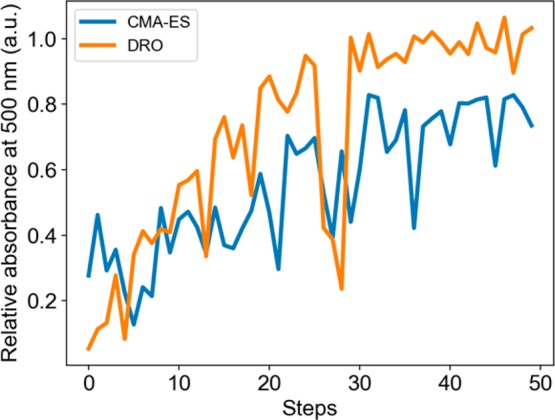
Performance comparison of CMA-ES and DRO on the bulk-phase reaction of silver nanoparticle synthesis.

Learning for Better Optimization

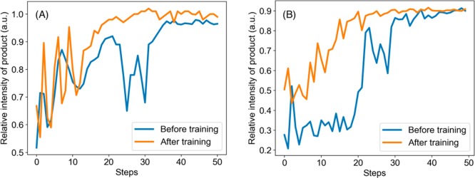
We also observed that the DRO algorithm is capable of learning while optimizing on real experiments. In other words, each time running a similar or even dissimilar reactions will improve the DRO policy. To demonstrate this point, the DRO was first trained on the reaction of the Pomeranz–Fritsch synthesis of isoquinoline and then tested on the reaction of the Friedländer synthesis of substituted quinoline. Figure 5A compares the performance of the DRO before and after training. The policy after training showed a better performance by reaching a higher yield at a faster speed.

Figure 5.

(A) The performance on Friedländer synthesis of DRO before and after training on the Pomeranz–Fritsch synthesis. (B) The performance on ribose phosphate synthesis of DRO before and after training on the Pomeranz–Fritsch and Friedländer syntheses.

The DRO policy showed better performance not only after training on a reaction with similar mechanism but also on reactions with different mechanisms. Figure 5B compares the performance of the DRO on ribose phosphate synthesis before and after training on the Pomeranz–Fritsch and Friedländer syntheses. Although they have achieved similar product yield, the DRO after training can reach the optimal condition with a faster speed.

Understanding the Reaction Mechanism

The reaction optimization process also provided us insights into the reaction mechanism. The reaction response surface was fitted by a Gaussian process (Figure 6), which showed that the yield at a low voltage of 1 kV was more sensitive to the pressure and flow rate change than the reaction at a higher voltage. On the other hand, the feature selection by Lasso^40,41 suggests that pressure/(flow rate), voltage/(flow rate), and square of pressure were the three most important features in determining the reaction yield. Flow rate and pressure were correlated because higher flow rate resulted in more liquid flowing out. In turn, the higher liquid flow needed higher pressure to generate smaller-sized droplets, in which reactions had a higher rate. The correlation was similar for voltage/(flow rate) pairs. Higher flow rate made the droplets larger; as a result, a higher voltage was required to generate enough charge to drive the reactions occurring inside them. The quadratic dependence on the pressure suggested that there was an optimal pressure for the reaction, because higher pressure would generate smaller-sized droplets with higher reaction rates, but smaller droplets would also evaporate faster; the faster evaporation would result in a shorter reaction time. The optimization process of DRO provides a better sampling than a grid search for LASSO regression. The DRO algorithm samples around the response surface with higher uncertainty, which reduces the bias of fitting. Besides, DRO also samples more around the optimal point, in order to get a more accurate fitting near the optimal. All of this data analysis leads us to a better understanding of how reactions occur in microdroplets.

Figure 6.

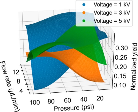
Possible reaction response surface of the Friedländer synthesis of a substituted quinoline, predicted from the optimization process.

Conclusion

We have developed the DRO model for optimizing chemical reactions and demonstrated that it has superior performance under a number of different circumstances. The DRO model combines state-of-the-art deep reinforcement learning techniques with the domain knowledge of chemistry, showcasing its capability in both speeding up reaction optimization and providing insight into how reactions take place in droplets. We suggest that the optimization strategy of integrating microdroplet reactions with our DRO acceleration can be applied to a wide range of reactions.

Experimental Details

Model Design

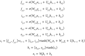
A modified long short-term memory (LSTM)⁴² architecture is proposed to accept two inputs of x_t–1 and y_t–1, and output the new x_t. The LSTM cell is defined as follows:

7

in which the variables are

• x_t–1, the input (reaction conditions) at time step t – 1;

• y_t–1, the output (reaction yield) at time step t – 1;

• c_t, the cell state vector;

• f_x,t, f_y,t, i_x,t, i_y,t, o_x,t, and o_y,t, gate vectors;

• W, U, and b, parameter matrices and vectors.

We denote elementwise multiplication by ◦ to distinguish it from matrix multiplication. The functions f, i, and o are named from forget, input, and output.

The proposed LSTM cell can be abbreviated as

8

In order to learn the optimal policy modeled by the RNN, we define a loss function inspired by the regret in reinforcement learning community as

9

where T is the overall time horizon, r_t is the reward at time step t, and γ ∈ (0, 1) is the discount factor. The term inside the parentheses measures the improvement we can achieve by exploration. The intuition of applying the discount factor is that the importance of getting a maximum reward increases as time goes on.

As mentioned before, chemical reactions are time-consuming to evaluate. Therefore, we need to train the model on mock reactions first. A class of nonconvex functions of the mixture Gaussian probability density functions is used as mock reactions, which allows a general policy to be trained. A Gaussian error term is added to the function to model the large variance property of chemical reaction measurements. The mock reactions can be written as

10

where c_i is the coefficient, μ_i is the mean, and Σ_i is the covariance of a multivariate Gaussian distribution; k is the dimension of the variables. is the error term, which is a random variable drawn from a Gaussian distribution with mean 0 and variance σ². In our case, the number of parameters to be optimized is three. N was set to 6. μ_i was sampled from a uniform distribution from 0.01 to 0.99, diagonalized Σ_i was sampled from a Gaussian distribution of , and the coefficient of c_i was sampled from a Gaussian distribution of and then normalized.

Training Details

The framework of tensorflow⁴³ is used to formulate and train the model. The LSTM structure is unrolled on trajectories of T = 50 steps, the nonconvex functions with random parameters in each batch are used as training sets, and the loss function (eq. 9) is used as the optimization goal. The Adam optimizer is used to train the neural network.

The hyperparameters chosen are “batch_size”, 128; “hidden_size”, 80; “num_layers”, 2; “num_epochs”, 50000; “num_params”, 3; “num_steps”, 50; “unroll_length”, 50; “learning_rate”, 0.001; “lr_decay”, 0.75; “optimizer”, “Adam”; “loss_type”, “oi”; and “discount_factor”, 0.97.

Chemicals and Instrumentation

All chemicals are purchased as MS grade from Sigma-Aldrich (St. Louis, MO). Mass spectra are obtained using an LTQ Orbitrap XL Hybrid Ion Trap-Orbitrap Mass Spectrometer from Thermo Fisher Scientific Inc. (Waltham, MA).

Experimental Setup

In the microdroplet reactions, reactant solutions from two syringes are mixed through a T-junction and sprayed in a desorption electrospray ionization source with application of high voltage and pressure. The reactions occur in droplets and are monitored by a mass spectrometer.

In the reaction of silver nanoparticle synthesis, sodium borohydride and trisodium citrate of specific concentrations were mixed and put into a bath at a specific temperature. Silver nitrate solution was then added dropwise. The concentration of AgNO₃ was fixed at 1 mM. The concentration of NaBH₄ ranged from 0.1 to 10 mM, the concentration of TSC ranged from 1 to 100 mM, and reaction temperature ranged from 25 to 100 °C.

Feature Selection by Lasso

Let p be the gas pressure, u be the voltage, and v be the flow rate. The engineered features are u, v, pu, pv, uv, p/u, p/v, u/v, p², u², v². The loss function of lasso regression is , where ∥•∥₂ is the 2 norm, ∥•∥₁ is the 1 norm, θ is the model parameter, x is the input features, y is the output results, and λ is the regularization coefficient. Features will pop out in an order corresponding to their importance when increasing the regularization coefficient while minimizing the loss function.¹³ Lasso regression is performed repeatedly so that exactly 1, 2, or 3 features are selected; the top three most important features are p/v, u/v, and p².

Data Availability

The corresponding code will be released on github.

The authors declare no competing financial interest.

References

- McMullen J. P.; Jensen K. F. Integrated Microreactors for Reaction Automation: New Approaches to Reaction Development. Annu. Rev. Anal. Chem. 2010, 3, 19–42. 10.1146/annurev.anchem.111808.073718. [DOI] [PubMed] [Google Scholar]
- Fabry D. C.; Sugiono E.; Rueping M. Self-Optimizing Reactor Systems: Algorithms, On-line Analytics, Setups, and Strategies for Accelerating Continuous Flow Process Optimization. Isr. J. Chem. 2014, 54, 341–350. 10.1002/ijch.201300080. [DOI] [Google Scholar]
- McMullen J. P.; Stone M. T.; Buchwald S. L.; Jensen K. F. An integrated microreactor system for self-optimization of a Heck reaction: from micro- to mesoscale flow systems. Angew. Chem., Int. Ed. 2010, 49, 7076–7080. 10.1002/anie.201002590. [DOI] [PubMed] [Google Scholar]
- Parrott A. J.; Bourne R. A.; Akien G. R.; Irvine D. J.; Poliakoff M. Self-Optimizing Continuous Reactions in Supercritical Carbon Dioxide. Angew. Chem., Int. Ed. 2011, 50, 3788–3792. 10.1002/anie.201100412. [DOI] [PubMed] [Google Scholar]
- Reizman B. J.; Wang Y.-M.; Buchwald S. L.; Jensen K. F. Suzuki–Miyaura cross-coupling optimization enabled by automated feedback. React. Chem. Eng. 2016, 1, 658–666. 10.1039/C6RE00153J. [DOI] [PMC free article] [PubMed] [Google Scholar]
- Plutschack M. B.; Pieber B.; Gilmore K.; Seeberger P. H. The Hitchhiker’s Guide to Flow Chemistry. Chem. Rev. 2017, 117, 11796–11893. 10.1021/acs.chemrev.7b00183. [DOI] [PubMed] [Google Scholar]
- Cortés-Borda D.; Kutonova K. V.; Jamet C.; Trusova M. E.; Zammattio F.; Truchet C.; Rodriguez-Zubiri M.; Felpin F.-X. Optimizing the Heck–Matsuda Reaction in Flow with a Constraint-Adapted Direct Search Algorithm. Org. Process Res. Dev. 2016, 20, 1979. 10.1021/acs.oprd.6b00310. [DOI] [Google Scholar]
- Echtermeyer A.; Amar Y.; Zakrzewski J.; Lapkin A. Self-optimization and model-based design of experiments for developing a C-H activation flow process. Beilstein J. Org. Chem. 2017, 13, 150–163. 10.3762/bjoc.13.18. [DOI] [PMC free article] [PubMed] [Google Scholar]
- Fitzpatrick D. E.; Battilocchio C.; Ley S. V. A Novel Internet-Based Reaction Monitoring, Control and Autonomous Self-Optimization Platform for Chemical Synthesis. Org. Process Res. Dev. 2016, 20, 386–394. 10.1021/acs.oprd.5b00313. [DOI] [Google Scholar]
- Holmes N.; Akien G. R.; Blacker A. J.; Woodward R. L.; Meadows R. E.; Bourne R. A. Self-optimization of the final stage in the synthesis of EGFR kinase inhibitor AZD9291 using an automated flow reactor. React. Chem. Eng. 2016, 1, 366–371. 10.1039/C6RE00059B. [DOI] [Google Scholar]
- Holmes N.; Akien G. R.; Savage R. J. D.; Stanetty C.; Baxendale I. R.; Blacker A. J.; Taylor B. A.; Woodward R. L.; Meadows R. E.; Bourne R. A. Online quantitative mass spectrometry for the rapid adaptive optimization of automated flow reactors. React. Chem. Eng. 2016, 1, 96–100. 10.1039/C5RE00083A. [DOI] [Google Scholar]
- Krishnadasan S.; Brown R. J. C.; deMello A. J.; deMello J. C. Intelligent routes to the controlled synthesis of nanoparticles. Lab Chip 2007, 7, 1434–1441. 10.1039/b711412e. [DOI] [PubMed] [Google Scholar]
- Sans V.; Porwol L.; Dragone V.; Cronin L. A self optimizing synthetic organic reactor system using real-time in-line NMR spectroscopy. Chemical Science 2015, 6, 1258–1264. 10.1039/C4SC03075C. [DOI] [PMC free article] [PubMed] [Google Scholar]
- LeCun Y.; Bengio Y.; Hinton G. Nature 2015, 521, 436–444. 10.1038/nature14539. [DOI] [PubMed] [Google Scholar]
- Rusk N. Nat. Methods 2015, 13, 35. 10.1038/nmeth.3707. [DOI] [Google Scholar]
- Duvenaud D. K.; Maclaurin D.; Iparraguirre J.; Bombarell R.; Hirzel T.; Aspuru-Guzik A.; Adams R. P. Convolutional Networks on Graphs for Learning Molecular Fingerprints. Neural Inf. Process. Syst. 2015, 2, 2224–2232. [Google Scholar]
- Hernández-Lobato J. M.; Requeima J.; Pyzer-Knapp E. O.; Aspuru-Guzik A. Parallel and Distributed Thompson Sampling for Large-scale Accelerated Exploration of Chemical Space. Proc. Mach. Learn. Res. 2017, 70, 1470–1479. [Google Scholar]
- Benjamin S.-L.; Carlos O.; Gabriel L. G.; Alan A.-G. Optimizing distributions over molecular space. An Objective-Reinforced Generative Adversarial Network for Inverse-design Chemistry (ORGANIC). ChemRxiv 2017, 10.26434/chemrxiv.5309668.v3. [DOI] [Google Scholar]
- Gómez-Bombarelli R.; Duvenaud D.; Hernández-Lobato J. M.; Aguilera-Iparraguirre J.; Hirzel T. D.; Adams R. P.; Aspuru-Guzik A.. Automatic chemical design using a data-driven continuous representation of molecules arXiv 2016; https://arxiv.org/abs/1610.02415v2. [DOI] [PMC free article] [PubMed]
- Kearnes S.; McCloskey K.; Berndl M.; Pande V.; Riley P. Molecular graph convolutions: moving beyond fingerprints. J. Comput.-Aided Mol. Des. 2016, 30, 595–608. 10.1007/s10822-016-9938-8. [DOI] [PMC free article] [PubMed] [Google Scholar]
- Altae-Tran H.; Ramsundar B.; Pappu A. S.; Pande V. Low Data Drug Discovery with One-Shot Learning. ACS Cent. Sci. 2017, 3, 283. 10.1021/acscentsci.6b00367. [DOI] [PMC free article] [PubMed] [Google Scholar]
- Coley C. W.; Barzilay R.; Jaakkola T. S.; Green W. H.; Jensen K. F. Prediction of Organic Reaction Outcomes Using Machine Learning. ACS Cent. Sci. 2017, 3, 434. 10.1021/acscentsci.7b00064. [DOI] [PMC free article] [PubMed] [Google Scholar]
- Wei J. N.; Duvenaud D.; Aspuru-Guzik A. Neural Networks for the Prediction of Organic Chemistry Reactions. ACS Cent. Sci. 2016, 2, 725–732. 10.1021/acscentsci.6b00219. [DOI] [PMC free article] [PubMed] [Google Scholar]
- Raccuglia P.; Elbert K. C.; Adler P. D. F.; Falk C.; Wenny M. B.; Mollo A.; Zeller M.; Friedler S. A.; Schrier J.; Norquist A. J. Machine-learning-assisted materials discovery using failed experiments. Nature 2016, 533, 73–76. 10.1038/nature17439. [DOI] [PubMed] [Google Scholar]
- Esteva A.; Kuprel B.; Novoa R. A.; Ko J.; Swetter S. M.; Blau H. M.; Thrun S. Dermatologist-level classification of skin cancer with deep neural networks. Nature 2017, 542, 115–118. 10.1038/nature21056. [DOI] [PMC free article] [PubMed] [Google Scholar]
- Eberlin L. S.; Tibshirani R. J.; Zhang J.; Longacre T. A.; Berry G. J.; Bingham D. B.; Norton J. A.; Zare R. N.; Poultsides G. A. Molecular assessment of surgical-resection margins of gastric cancer by mass-spectrometric imaging. Proc. Natl. Acad. Sci. U. S. A. 2014, 111, 2436–2441. 10.1073/pnas.1400274111. [DOI] [PMC free article] [PubMed] [Google Scholar]
- Zhou Z.; Zare R. N. Personal Information from Latent Fingerprints Using Desorption Electrospray Ionization Mass Spectrometry and Machine Learning. Anal. Chem. 2017, 89, 1369–1372. 10.1021/acs.analchem.6b04498. [DOI] [PubMed] [Google Scholar]
- The CMA Evolution Strategy: A Comparing Review In Towards a New Evolutionary Computation; Springer-Verlag: Berlin/Heidelberg, 2006; pp 75–102. [Google Scholar]
- Nelson L. S.Nelder-Mead Simplex Method. In Encyclopedia of Statistical Sciences; John Wiley & Sons, Inc: Hoboken, NJ, 2004. [Google Scholar]
- Huyer W.; Neumaier A. SNOBFIT – Stable Noisy Optimization by Branch and Fit. ACM Transactions on Mathematical Software 2008, 35, 1–25. 10.1145/1377612.1377613. [DOI] [Google Scholar]
- Lee J. K.; Banerjee S.; Nam H. G.; Zare R. N. Acceleration of reaction in charged microdroplets. Q. Rev. Biophys. 2015, 48, 437–444. 10.1017/S0033583515000086. [DOI] [PMC free article] [PubMed] [Google Scholar]
- Yan X.; Bain R. M.; Cooks R. G. Organic Reactions in Microdroplets: Reaction Acceleration Revealed by Mass Spectrometry. Angew. Chem., Int. Ed. 2016, 55, 12960–12972. 10.1002/anie.201602270. [DOI] [PubMed] [Google Scholar]
- Banerjee S.; Gnanamani E.; Yan X.; Zare R. N. Can all bulk-phase reactions be accelerated in microdroplets?. Analyst 2017, 142, 1399–1402. 10.1039/C6AN02225A. [DOI] [PubMed] [Google Scholar]
- Osband I., Van Roy B., Wen Z.. Generalization and Exploration via Randomized Value Functions. In Proceedings of the 33rd International Conference on Machine Learning; 2016; pp 2377–2386; JMLR.org.
- Florensa C., Duan Y., Abbeel P.. Stochastic Neural Networks for Hierarchical Reinforcement Learning. CoRR abs/1704.03012;2017 [Google Scholar]
- Banerjee S.; Zare R. N. Syntheses of Isoquinoline and Substituted Quinolines in Charged Microdroplets. Angew. Chem., Int. Ed. 2015, 54, 14795–14799. 10.1002/anie.201507805. [DOI] [PubMed] [Google Scholar]
- Nam I.; Lee J. K.; Nam H. G.; Zare R. N. Abiotic production of sugar phosphates and uridine ribonucleoside in aqueous microdroplet. Proc. Natl. Acad. Sci. U. S. A. 2017, 114, 12396–12400. 10.1073/pnas.1714896114. [DOI] [PMC free article] [PubMed] [Google Scholar]
- Lee J. K.; Kim S.; Nam H. G.; Zare R. N. Microdroplet fusion mass spectrometry for fast reaction kinetics. Proc. Natl. Acad. Sci. U. S. A. 2015, 112, 3898–3903. 10.1073/pnas.1503689112. [DOI] [PMC free article] [PubMed] [Google Scholar]
- Iravani S.; Korbekandi H.; Mirmohammadi S. V.; Zolfaghari B. Synthesis of silver nanoparticles: chemical, physical and biological methods. Res. Pharm. Sci. 2014, 9, 385–406. [PMC free article] [PubMed] [Google Scholar]
- Tibshirani R. Regression Shrinkage and Selection Via the Lasso. J. R. Stat. Soc., Ser. B 1994, 58, 267–288. [Google Scholar]
- Tibshirani R. The Lasso Method for Variable Selection in the Cox Model. Statist. Med. 1997, 16, 385–395. . [DOI] [PubMed] [Google Scholar]
- Hochreiter S.; Schmidhuber J. Long Short-Term Memory. Neural Computation 1997, 9, 1735–1780. 10.1162/neco.1997.9.8.1735. [DOI] [PubMed] [Google Scholar]
- Abadi M.; Agarwal A.; Barham P.; Brevdo E.; Chen Z.; Citro C.; Corrado G. S.; Davis A.; Dean J.; Devin M.; Ghemawat S.; Goodfellow I. J.; Harp A.; Irving G.; Isard M.; Jia Y.; Józefowicz R.; Kaiser L.; Kudlur M.; Levenberg J.; Mané D.; Monga R.; Moore S.; Murray D. G.; Olah C.; Schuster M.; Shlens J.; Steiner B.; Sutskever I.; Talwar K.; Tucker P. A.; Vanhoucke V.; Vasudevan V.; Viégas F. B.; Vinyals O.; Warden P.; Wattenberg M.; Wicke M.; Yu Y.; Zheng X.. TensorFlow: Large-Scale Machine Learning on Heterogeneous Distributed Systems. CoRR abs/1603.04467; 2016 [Google Scholar]
Associated Data
This section collects any data citations, data availability statements, or supplementary materials included in this article.
Data Availability Statement