An Adaptive Approach to Locating Mobile HIV Testing Services

Abstract

Background

Public health agencies suggest targeting “hotspots” to identify individuals with undetected HIV infection. However, definitions of hotspots vary. Little is known about how best to target mobile HIV testing resources.

Methods

We conducted a computer-based tournament to compare the yield of four algorithms for mobile HIV testing. Over 180 rounds of play, algorithms selected one of three hypothetical zones, each with unknown prevalence of undiagnosed HIV, in which to conduct a fixed number of HIV tests. The algorithms were: 1) Thompson Sampling, an adaptive Bayesian search strategy; 2) Explore-then-Exploit, a strategy that initially draws comparable samples from all zones and then devotes all remaining rounds of play to HIV testing in whichever zone produced the highest observed yield; 3) Retrospection, a strategy using only base prevalence information; and; 4) Clairvoyance, a benchmarking strategy that employs perfect information about HIV prevalence in each zone.

Results

Over 250 tournament runs, Thompson Sampling outperformed Explore-then-Exploit 66% of the time, identifying 15% more cases. Thompson Sampling’s superiority persisted in a variety of circumstances examined in sensitivity analysis. Case detection rates using Thompson Sampling were, on average, within 90% of the benchmark established by Clairvoyance. Retrospection was consistently the poorest performer.

Limitations

We did not consider either selection bias (i.e., the correlation between infection status and the decision to obtain an HIV test) or the costs of relocation to another zone from one round of play to the next.

Conclusions

Adaptive methods like Thompson Sampling for mobile HIV testing are practical and effective, and may have advantages over other commonly used strategies.

Introduction

The Centers for Disease Control and Prevention (CDC) estimate that fourteen percent of the 1.2 million individuals in the United States (US) living with HIV infection are undiagnosed(1)(2). The clinical and public health importance of this population is profound. As many as two-thirds of new HIV transmissions may be attributable to individuals who are unaware of their HIV infection(3)(4)(5). Moreover, undiagnosed individuals initiate antiretroviral therapy later in their disease, compromising their health and well-being(6). This phenomenon is also global: for instance, in sub-Saharan Africa, the majority of HIV+ individuals do not know their HIV status(7)(8).

Improving the yield of HIV testing programs remains a research priority(9). Sophisticated targeting, tracing and testing methods have been proposed to identify recent infections from the same source by phylogenetic or social network analysis (9)(10)(11). Specific approaches focusing on “hotspots” of undiagnosed HIV infection have been widely discussed, stressing the need to focus testing efforts in targeted areas(9)(12)(13). Yet, how to define best an HIV “hotspot” remains an open question. Convenient proxy measures (e.g., prior estimates of disease prevalence or demographic characteristics) have proven to be poor at predicting which locales and groups may have high density of undiagnosed HIV(14)(15).

Mobile HIV testing using vans or other forms of community outreach are widely used to supplement testing at fixed sites and has been promoted by the CDC and the World Health Organization (WHO)(16)(17). Mobile testing can be particularly effective in reaching some of the highest-risk populations(16)(18)(19). However, practitioners often rely on subjective recommendations from local public health officials, the staff of testing programs, and clients who have received testing services in the past to make decisions about where to test in outreach and community based settings(16). Mobile testing units frequently target areas where the prevalence of HIV or AIDS was high when last estimated (20) (Stonehouse P., Chicago Department of Health, personal communication). We know of no research on how to optimize the deployment of mobile HIV testing services.

The question of where to target HIV testing can be usefully portrayed as an exploration-exploitation dilemma, a classic problem in the field of sequential decision making under uncertainty(21). The decision maker who seeks to maximize long-run gains must strike a balance between: deploying resources to improve knowledge of the prevailing circumstances; and then make the best possible use of whatever is already known about the current circumstances. Bandit algorithms are named for one-armed bandits (slot machines) and the choices a gambler must make in deciding which machines to play, for how often, and in which sequence to maximize winnings after observing the payouts from the machines played in the past. These algorithms provide a systematic way of solving exploitation-exploration problems(22). While bandit methods have been applied successfully to problems in fields ranging from military searches to oilfield exploration and online advertising, their use in the realm of public health and medical practice is limited(23)(24)(25)(26)(27). This study assessed the effectiveness and efficiency of several strategies, including a bandit algorithm, for targeting mobile HIV testing, under conditions similar to those encountered in urban epidemics with different proportions of undiagnosed cases of HIV infection.

Methods

Analytic Overview

We conducted a computer-based tournament to compare the performance of four approaches to targeted mobile HIV testing in a hypothetical setting consisting of several geographic zones, each with unknown prevalence of undetected HIV infection. In each round of play, a strategy was required to designate a single zone in which to conduct a fixed number of HIV tests. Prior to each round of play, the strategy was permitted to assess the results of its testing activities in prior rounds. Performance was measured by the total number of HIV cases newly detected by a given strategy over multiple rounds of play. A secondary outcome was the magnitude of a strategy’s average margin of success in finding new cases over other strategies.

HIV Infection and Geographic Zones

For the main analysis, we assumed that there were three zones (i ∈ {1,2,3}) and T = 180 rounds of play, hereinafter referred to as days (reflecting the ease and plausibility with which mobile testing facilities can be relocated from one day to the next). Prior to the first day, we initialized the simulation by assigning different numbers of infected and uninfected persons (denoted by U_i(0) and I_i(0), respectively) to each zone. These were further separated into observed infected OI_i(0) and unobserved infected UI_i(0) individuals, while the uninfected population was composed of observed uninfected OU_i(0) and unobserved uninfected UU_i(0) individuals. This gave rise to two useful measures of prevalence: $\frac{I_i(t)}{I_i(t)+U_i(t)}$, the population prevalence of HIV infection in zone i on day t; and $\frac{{\mathit{UI}}_i(t)}{{\mathit{UI}}_i(t)+{\mathit{UU}}_i(t)}$, the prevalence of HIV infection in zone i among persons whose HIV infection status is unknown on day t (which we label the undiagnosed prevalence, UP_i(t).)

The undiagnosed prevalence UP_i(t) value was used to determine the results of HIV testing on each day. If m HIV tests were conducted in zone i on day t, we determined the number of newly identified cases, X_i(t), by sampling m times from a binomial probability distribution with success probability UP_i(t). This reflects the simplifying assumption that tests were only conducted on persons whose HIV-infection status was unknown. It also reflects the simplifying assumption of sampling with replacement, that is, UP_i(t) was established at the beginning of day t and remained unaltered by any screening that took place in that zone i on that day. (In reality, every HIV test produces an instantaneous change in the underlying prevalence of undetected infection. Our simplification is justified so long as the number of tests m conducted on a given day and in a given zone i was far smaller than the number of unobserved infections UI_i(t) in that zone.) At the end of each day, we updated the unobserved prevalence to:

$${\mathit{UP}}_i(t+1)=\frac{{\mathit{UI}}_i(t)-X_i(t)}{[{\mathit{UI}}_i(t)-X_i(t)]+[{\mathit{UU}}_i(t)-(m-X_i(t))]}.$$

Underlying undiagnosed prevalence UP_i(t) was assumed to change in two additional ways: 1) observed uninfected individuals could return to the pool of unobserved uninfected individuals after a specified period, reflecting the declining reliability and relevance of a negative result with the passage of time; and 2) new arrivals (both unobserved-infected and unobserved-uninfected) could enter the population.

Strategy 1: Thompson Sampling (TS)

TS is a Bayesian approach that simultaneously explores and exploits, choosing the course of action that maximizes expected future rewards based on random sampling from probability distributions that are themselves based upon prior probability distributions and observation(28)(29)(30). TS is distinguished from the other strategies by: a) updating probabilities about the prevalence of undetected HIV infection, based on the observed results of its HIV testing activities; and b) use of randomization to choose a zone based on those probabilities. Prior to the first day of play, the TS algorithm employs a Beta(α_i, β_i) probability distribution for the prevalence of undiagnosed HIV among individuals in zone i at time t=0. The Beta distribution is a continuous distribution on the interval (0,1) and is conjugate to the binomial distribution (i.e., the posterior distribution is beta when the likelihood is binomial and the prior is beta).

TS selects a zone i for testing, prior to each day, by sampling from each zone’s current probability distribution for undetected HIV prevalence and then choosing the zone with the largest value. TS makes its selection without sampling from the zones themselves; rather, sampling is conducted on the undetected HIV prevalence distributions for each zone. Every zone has a non-zero probability of being selected for testing on any given day; but the probability that a given zone will be selected is aligned with prior estimates about the prevalence of undetected HIV infection in that zone. Once a zone is selected for testing on a given day, testing commences in that zone. The results of the tests from that day are used to update the probabilities for that zone: if the process of screening m persons in zone i on the first day produces x new cases detected, the posterior probability will follow a Beta (α_i + x, β_i + (m-x)) distribution. This updated distribution becomes the sampling distribution for zone selection for the second day (see Appendix for more details).

Strategy 2: Explore-then-Exploit (ETE)

This algorithm splits the total number of days of play in two: an initial, exploratory phase (number of zones times t_explore), during which ETE samples in equal measures from all zones; and a subsequent exploitation phase, during which ETE devotes all remaining days to HIV testing in whichever zone produced the highest observed yield during the exploratory phase. This is in contrast to TS, which explores and exploits on an ongoing, adaptive basis. There is some flexibility in the number of days ETE may devote to exploration; more days dedicated to initial sampling increases the algorithm’s power to detect the most promising zone but reduces the number of days remaining to exploit that information. We considered alternative exploratory periods in sensitivity analysis. Once the initial exploration period is over and a zone has been chosen for the exploitation phase, the ETE strategy stops “learning” and never “changes its mind”, no matter how poorly it subsequently performs in its selected zone.

Strategy 3: Retrospection

The literature suggests that many jurisdictions deploy their mobile HIV testing resources based on historical information about where the greatest number of new cases of HIV infection were identified in the past(20) (Stonehouse P., Chicago Department of Health, personal communication). The Retrospection strategy thus always chooses the zone with the highest previously estimated HIV prevalence for testing on any given day.

Strategy 4: Clairvoyance

The Clairvoyance strategy has access to perfect information about the prevalence of undiagnosed HIV infection in each geographic area on every day. The performance of this strategy provides an upper-bound benchmark of what could be achieved by testing only in the zone with the highest actual prevalence of undiagnosed HIV infection on any given day(24). The Clairvoyance strategy only has perfect information about the prevalence of undetected HIV infection in a given zone; it does not have any special knowledge about the HIV-infection status of individuals within that zone. Thus, it can select the most promising zone within which to conduct HIV screening activities but it cannot guarantee that individuals selected for screening within that zone will be infected (that is, the strategy samples with replacement on all individuals regardless of actual infection status).

Parameter Definitions, Main Analysis and Sensitivity Analyses

Initial parameter values as well as those used in the sensitivity analyses are described in Tables 1 and 2. We did not base the parameter values on data from a specific region or country, choosing instead to understand how the four strategies described above would perform in a variety of circumstances. We explored values ranging from 0.05% to 6.75%, for the underlying prevalence of undiagnosed HIV infection. The low value reflects epidemics, like those in the US, where overall HIV prevalence is low and most (>85%) people know their HIV status, while the higher value represents epidemics where HIV prevalence is high as are undiagnosed infections, such as in South Africa (1)(2)(31)(32). We assumed there was no correlation between estimated HIV prevalence in a previous year and the current prevalence of undiagnosed HIV infection in each zone. We made this assumption because high prevalence in and of itself does not indicate that a location has a high number of undiagnosed individuals. Settings with older epidemics and successful testing programs (New York State, for example) may have many HIV-infected individuals but few individuals with undiagnosed HIV infection (33). In addition, several authors have described the limitations of using prevalence surveys and the lack of consensus on how best to locate undiagnosed cases (34)(35). Finally, estimating prevalence in geographic areas with small numbers of people in the at-risk population can be challenging (36). For these reasons, we did not use previous year’s HIV prevalence in a zone as a one-to-one surrogate for the current year’s prevalence of undiagnosed HIV infection. However, if the estimated HIV prevalence did correlate with the prevalence of undiagnosed HIV infection, the Retrospection strategy would perform as a partial Clairvoyance strategy, knowing the rank order of zones to test in on the first day of the simulation, but being unable to account for shifts in the underlying prevalence on subsequent days.

Table 1.

Parameter Main Analysis Values

Parameters	Values
	Zone 1	Zone 2	Zone 3
Overall Population	56521	54991	56362
Previous Year’s HIV Prevalence	2.43%	2.41%	1.88%
Underlying Prevalence of Undiagnosed HIV Infection	1.50%	2.25%	3.38%
New Infections/day	1.0	0.68	0.45
New HIV- Arrivals/day	5	7.5	11.25
Days Until Return to Unobserved, Uninfected Pool	45	45	45
Initial Number of Days for Sampling for Explore-Then-Exploit Strategy	30 (all zones)
Days of Testing (Duration of Simulation)	180 (all zones)
Initial Observed HIV+/HIV− (Priors)	Beta(1,1)
Tests Per Day	25(all zones)

Table 2.

Parameter Values for Sensitivity Analysis

Parameters	Values
	Zone 1	Zone 2	Zone 3
Low, Underlying Prevalence of Undiagnosed HIV Infection	0.05%	0.08%	0.11%
High, Underlying Prevalence of Undiagnosed HIV Infection	3.0%	4.5%	6.75%
Low, New Infections/day	0	0	0
High, New Infections/day	3.38	2.25	1.5
Low, New HIV-Arrivals/day	0	0	0
High, New HIV-Arrivals/day	10	15	22.5
Low, Days Until Return to Unobserved, Uninfected Pool	10	10	10
High, Days Until Return to Unobserved, Uninfected Pool	90	90	90
Low, Initial Number of Days for Sampling for Explore Then Exploit Strategy	5 (all zones)
High, Initial Number of Days for Sampling for Explore Then Exploit Strategy	45 (all zones)
Low-Days Testing (Duration of Simulation)	100 (all zones)
High-Days of Testing (Duration of Simulation)	1000 (all zones)
Informative Prior for Thompson Sampling Strategy (sample size=10)	Beta(0.1,9.9)
Informative Prior for Thompson Sampling Strategy (sample size=100)	Beta(1,99)
Low, Tests Per Day	10 (all zones)
High, Tests Per Day	40 (all zones)

We considered different rates of population movement, setting in-migration of new HIV-negative individuals between 5–12 per day in each zone in the main analysis, to reflect fast-growing settings. We also considered a case with no in-migration in the sensitivity analysis. We chose 45 days as the baseline “shelf life” of an HIV-negative test result, after which the observed negative case returned to the unobserved, uninfected pool(37)(38). We chose 180 days (range: 100 – 1000) for the main analysis number of days of testing, to represent a mid-year review of the strategy for a hypothetical decision maker who might be evaluating new approaches for targeting HIV testing. In the main analysis, the number of tests per day (m) was set at 25; we explored values from 10 to 40 tests per day in sensitivity analysis (18)(39). In the main analysis, zones were assigned HIV incidence rates ranging from 0.5–1 infections per day; we considered values from 0 to 3.5 in sensitivity analysis, reflecting static epidemics and ones where incidence is still high(40).

We chose a value of 30 days of exploration in each zone in the main analysis for the ETE strategy. This period was selected to represent the number of days a decision maker might be willing to defer a choice about a testing program’s location. In the sensitivity analyses, we examine values ranging from 5 to 45 days, to represent decision makers who have varying degrees of flexibility or patience in terms of making choices about deployment of resources. If we had required the ETE strategy to base its decision on a sample size calculation with assumptions about power (e.g. 1-β=0.90) and significance or Type I error probability (e.g. α=0.05) and adjusted for multiple comparisons using the same historical data on HIV prevalence figures used by the Retrospection strategy as baseline predictions, the exploratory phase would have exceeded 1800 rounds of play.

For the TS strategy, we applied uniform, uninformative Beta(α=1,β=1) distributions to represent prior beliefs about the underlying prevalence of HIV infection in all three zones. This permitted us to evaluate TS in a setting where we have virtually no information about the prevalence of undiagnosed HIV infection in any of the zones. Of course, there is a great deal of existing information about the AIDS epidemic in the US and in other countries, which would allow us to construct more informative prior probabilities. To that end, in the sensitivity analyses, we evaluated TS with two other Beta distributions common across all zones: Beta (0.1, 9.9) and Beta (1, 99), both of which assume a mean prevalence of undiagnosed HIV infection across all the zones of 1% with sample sizes of 10 and 100, respectively. This 1% figure was chosen based on an assumption that the prevalence of unobserved HIV+ individuals in each zone is less than the existing HIV prevalence(41).

We ran the tournament 250 times with any given set of data assumptions. All performance statistics reported in the next section represent averages across these 250 runs. If a strategy outperformed another in a head-to-head comparison with greater than or equal to 55.25% of the wins in 250 simulations, we reported this result as significant. This 55.25% figure was derived from a one-sided Z-test of a difference in proportions, where 0.5525 is the threshold for a difference in proportions with a p-value of less than 0.05.

Results

Main Analysis

In the main analysis, Clairvoyance outperformed all other strategies in overall number of new HIV diagnoses. TS (and ETE) identified 90% (and 84%) as many new infections as Clairvoyance, while Retrospection found just 50% (Figure 1). In a head-to-head comparison, TS outperformed ETE 65.9% of the time, with an average margin of victory of 18.6 new cases; in the 31.7% of instances where ETE outperformed TS, the margin of victory averaged 13.2 new cases (see Figure 2; there were some ties so values do not sum to 100%).

Figure 1.

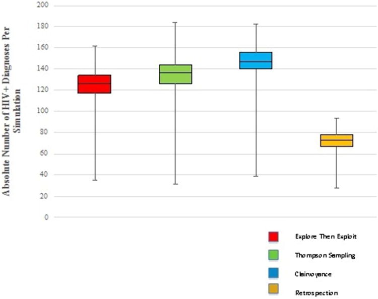
Basic statistics for all four strategies: number of HIV+ diagnoses.

Figure 2.

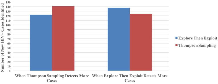
Magnitude of loss in head-to-head comparison of Thompson sampling versus explore-then-exploit strategy.

Sensitivity Analysis

We re-evaluated all findings using the data ranges specified in Tables 1 and 2. Generally, overall win percentages and average margins of victory remained stable under the tested parameter values (Table 3). However, the win differential between ETE and TS vanished when any of the following changes were made: the overall prevalence of undetected HIV in the population was reduced below 1%; the prevalence differential between zones was reduced; or fewer than 10 tests were performed per day. ETE and TS also had no significant difference (p>0.05) in wins when we increased the number of days of testing above 1000; here however, TS’s average margin of victory against ETE was far larger than ETE’s average margin of victory against TS.

Table 3.

Results for Main Analysis Values and Sensitivity Analysis for Thompson Sampling vs. Explore Then Exploit Strategies Only

Parameters	Values
	Zone 1	Zone 2	Zone 3	Percentage of Time TS Outperforms ETE Over 250 Repetitions of Simulation (TS finds more HIV+ cases)	Percentage of Time ETE Outperforms TS Over 250 Repetitions of Simulation (ETE finds more HIV+ cases)	Percentage of Time ETE Ties TS Over 250 Repetitions of Simulation	Mean Number of Cases Detected by TS (when TS finds more cases than ETE)	Standard Deviation of Number of Cases Detected by TS (when TS finds more cases than ETE)	Mean Number of Cases Detected by ETE (when TS finds more cases than ETE)	Standard Deviation of Number of Cases Detected by ETE (when TS finds more cases than ETE)	Mean Number of Additional Cases Detected Over ETE (when TS finds more HIV+ cases than ETE)	Mean Number of Cases Detected by ETE (when ETE finds more cases than TS)	Standard Deviation of Number of Cases Detected by ETE (when ETE finds more cases than TS)	Mean Number of Cases Detected by TS (when ETE finds more cases than TS)	Standard Deviation of Number of Cases Detected by TS (when ETE finds more cases than TS)	Mean Number of Additional Cases Detected Over TS (when ETE finds more HIV+ cases than TS)	Difference in Number of Cases Detected by Each Outperforming Strategy
Main analysis Underlying Probability of Success	1.50%	2.25%	3.38%	65.86%**	31.73%	2.41%	140.77	11.52	122.21	10.83	18.55	137.71	9.66	124.56	12.23	13.15	5.40
(vary value in zone 1)
Underlying Probability of Success (lower value than main analysis)	0.05%	0.08%	0.11%	47.20%	42.00%	10.80%	10.15	2.52	6.54	2.09	3.61	10.01	2.71	6.53	2.32	3.48	0.13
Underlying Probability of Success (higher value than main analysis)	3.00%	4.50%	6.75%	81.93%**	17.27%	0.80%	282.45	16.82	246.21	17.70	36.25	265.67	13.72	248.72	21.58	16.95	19.29
(vary spread-main analysis medium spread between zones)
Underlying Probability of Success (no spread between zones)	1.50%	1.50%	1.50%	47.01%	50.60%	2.39%	74.78	7.51	66.02	6.83	8.76	75.20	6.20	67.45	6.30	7.75	1.01
Underlying Probability of Success (large spread between zones)	1.50%	3.75%	9.38%	100.00%**	0.00%	0.00%	391.25	20.21	313.54	16.89	77.71	N/A	N/A	N/A	N/A	N/A	N/A
Main analysis New Infections/day	1.0125	0.675	0.45	65.86%**	31.73%	2.41%	140.77	11.52	122.21	10.83	18.55	137.71	9.66	124.56	12.23	13.15	5.40
(vary value in zone 3)
New Infections/day (lower value than main analysis)	0	0	0	62.80%**	32.80%	4.40%	136.83	11.59	116.66	11.66	20.17	132.65	8.68	119.54	10.83	13.11	7.06
New Infections/day (higher value than main analysis)	3.38	2.25	1.5	65.86%**	32.13%	2.01%	147.21	10.69	128.57	11.68	18.64	142.04	10.68	130.53	12.34	11.51	7.13
(vary spread-main analysis medium spread between zones)
New Infections/day (no spread between zones)	0.45	0.45	0.45	67.87%**	29.32%	2.81%	139.73	11.77	120.77	12.69	18.95	135.07	8.32	123.85	10.21	11.22	7.73
New Infections/day (large spread between zones)	2.8125	1.125	0.45	63.86%**	34.54%	1.61%	138.06	11.21	121.52	11.96	16.54	137.49	10.72	122.93	11.39	14.56	1.98
Main analysis New HIV-Arrivals/day	5	7.5	11.25	65.86%**	31.73%	2.41%	140.77	11.52	122.21	10.83	18.55	137.71	9.66	124.56	12.23	13.15	5.40
(vary value in zone 1)
New HIV-Arrivals/day (lower value than main analysis)	0	0	0	63.86%**	33.33%	2.81%	140.79	9.85	124.47	11.28	16.32	137.96	10.21	124.56	12.44	13.40	2.92
New HIV-Arrivals/day (higher value than main analysis)	10	15	22.5	62.15%**	35.06%	2.79%	138.39	10.95	120.06	11.81	18.32	133.43	9.39	118.84	11.64	14.59	3.73
(vary spread-main analysis medium spread between zones)
New HIV-Arrivals/day (no spread between zones)	5	5	5	66.27%**	32.53%	1.20%	141.50	11.89	122.02	10.94	19.48	135.98	10.44	122.41	12.22	13.56	5.92
New HIV-Arrivals/day (large spread between zones)	5	12.5	31.25	61.45%**	35.74%	2.81%	135.13	12.02	117.11	11.13	18.01	132.26	9.24	118.37	11.25	13.89	4.13
Main analysis Days Until Return to Unobserved, Uninfected Pool	45	45	45	65.86%**	31.73%	2.41%	140.77	11.52	122.21	10.83	18.55	137.71	9.66	124.56	12.23	13.15	5.40
(vary value in zone 1)
Days Until Return to Unobserved, Uninfected Pool (lower value than main analysis)	10	10	10	63.86%**	34.14%	2.01%	139.10	11.91	120.18	11.98	18.92	134.85	9.49	122.11	11.86	12.74	6.18
Days Until Return to Unobserved, Uninfected Pool (higher value than main analysis)	90	90	90	64.66%**	33.33%	2.01%	139.08	11.31	120.93	12.34	18.15	135.07	9.57	123.99	10.65	11.08	7.07
(vary spread-main analysis no spread between zones)
Days Until Return to Unobserved, Uninfected Pool (medium spread between zones)	45	67.5	101.25	66.67%**	31.33%	2.01%	142.25	10.43	123.45	11.67	18.80	137.42	9.29	125.06	11.79	12.36	6.44
Days Until Return to Unobserved, Uninfected Pool (large spread between zones)	45	90	180	66.27%**	30.12%	3.61%	141.48	11.33	121.73	13.75	19.76	135.25	10.50	121.65	13.15	13.60	6.16
Main analysis Initial Number of Days for Sampling for ETE Strategy	30 (all zones)			65.86%**	31.73%	2.41%	140.77	11.52	122.21	10.83	18.55	137.71	9.66	124.56	12.23	13.15	5.40
Initial Number of Days for Sampling for ETE Strategy (lower value than main analysis)	5 (all zones)			56.63%**	42.57%	0.80%	137.68	14.35	104.02	22.85	33.66	146.81	11.47	128.17	13.22	18.64	15.02
Initial Number of Days for Sampling for ETE Strategy (higher value than main analysis)	45 (all zones)			77.51%**	20.08%	2.41%	137.14	11.91	115.45	9.78	21.68	126.28	9.62	115.88	10.67	10.40	11.28
Main analysis Days of Testing (Duration of Simulation)	180 (all zones)			65.86%**	31.73%	2.41%	140.77	11.52	122.21	10.83	18.55	137.71	9.66	124.56	12.23	13.15	5.40
Days of Testing (Duration of Simulation) (lower value than main analysis)	100 (all zones)			77.60%**	21.60%	0.80%	74.74	8.77	60.28	7.24	14.46	68.24	6.57	60.63	6.61	7.61	6.84
Days of Testing (Duration of Simulation) (higher value than main analysis)	1000 (all zones)			55.02%	44.98%	0.00%	727.19	21.14	675.71	59.42	51.48	725.43	18.78	703.05	18.48	22.38	29.10
Main analysis Observed HIV+/HIV− Priors	Beta (1,1) (all zones)			65.86%**	31.73%	2.41%	140.77	11.52	122.21	10.83	18.55	137.71	9.66	124.56	12.23	13.15	5.40
Informative Priors (N=10)	Beta (0.1, 9.9) (all zones)			65.06%**	33.33%	1.61%	144.67	11.25	123.20	11.47	21.47	133.72	11.33	115.72	18.17	18.00	3.47
Informative Priors (N=100)	Beta (1, 99) (all zones			69.08%**	29.32%	1.61%	142.77	12.46	119.98	13.41	22.80	134.44	9.43	120.88	14.03	13.57	9.23
Main analysis Tests Per Day	25 (all zones)			65.86%**	31.73%	2.41%	140.77	11.52	122.21	10.83	18.55	137.71	9.66	124.56	12.23	13.15	5.40
T ests Per Day (lower value than main analysis)	10 (all zones)			51.81%	43.37%	4.82%	56.16	7.02	45.12	7.61	11.05	55.59	6.22	44.95	7.06	10.64	0.41
T ests Per Day (higher value than main analysis)	40(all zones)			73.90%**	25.30%	0.80%	222.22	13.09	198.45	15.85	23.78	216.00	10.21	202.52	13.85	13.48	10.29

^**Significant (in green) one-sided z-test with p<0.05 (95% CI).

The performance of TS was improved when it employed more informative priors with larger sample sizes: using prior belief distributions Beta (1, 99) increased its win percentage against ETE from 65.8% to 69.1%. The performance of ETE was improved when it spent fewer days in the initial “exploratory” phase. When ETE sampled for 5 days (rather than 30 days) in each zone, its win percentage rose from 31.7% to 42.6%. However, less exploration also introduced greater volatility into ETE’s performance, increasing its average margins of both wins and losses.

Discussion

In the literature, more complex bandit approaches have been discussed in the context of clinical trial design, the allocation of resources from the national strategic stockpile for influenza outbreaks and the design of mHealth apps (42)(43)(44)(45)(46). We know of no work that has used Thompson Sampling or other bandit algorithms to improve the performance of mobile HIV testing or to operationalize the focus on hotspots of HIV, or to improve the detection and diagnosis of other infectious or chronic diseases. However, other approaches to sequential decision making under uncertainty, of which bandit algorithms are a part, such as adaptive sampling and Markov decision processes, have been explored in health(47)(48). Our results suggest that TS is a practical and effective approach to locating high-yield locations for HIV testing. TS outperformed ETE in the main analysis and in all but a few circumstances in the sensitivity analysis and detected only 10% fewer cases than could be achieved using a benchmark Clairvoyance strategy with access to perfect information. The performance of TS in the main analysis is consistent with evaluations of TS versus similar explore-then-exploit approaches in the sequential decision making literature(28)(30). In fact, evidence that TS performs better as the number of arms increases in an experiment suggests that the head-to-head superiority of TS against ETE should increase with additional geographic zones in the simulation(43)(49)(50).

Sensitivity analyses indicate that TS performs best when geographic zones differ greatly in their prevalence of undetected HIV. Importantly, when the underlying prevalence of undiagnosed HIV infection is low, all strategies perform poorly. This may make TS less useful in the general population in the US, where relatively few people are living with undiagnosed HIV infection, and more appropriate for wide use in countries with more severe epidemics. This also suggests that TS may be particularly suited to communities in the US and elsewhere, where HIV infection is thought to be heterogeneously distributed and “hotspots” are believed to exist. TS could be targeted to assist in choosing among locations (e.g. gay social venues), where prevalence and/or incidence may be higher than in the general population and where risk among these special locations varies as well(51)(52)(53). A particularly attractive feature of the TS algorithm is its simplicity of implementation and the ease with which it can be updated in real time. At the end of each day, the staff need only make note of the zone visited, the number of tests performed, and the number of new cases detected.

Our study has several limitations. We considered only three zones for HIV testing; in reality, decision makers must often choose from among large numbers of possible locations. We conceived of zones as distinct geographical areas; in practice, “hotspots” may have both a geographic and a temporal component (e.g., an area with many nightclubs may only be a hotspot late on Fridays and Saturdays). And we did not account for potential correlations between adjacent zones in their prevalence of undetected HIV, although this would not be a factor in our example that used only three zones. We also did not account for the possibility of differential rates of uptake in testing within zones. For example, it is possible that there is a correlation between risk of infection (or infection status) and an individual’s decision to obtain an HIV test. While we opted for simplicity in our assessment of mobile HIV testing, our approach is flexible enough to accommodate the elaborations discussed above and to adapt to more complicated forms of immigration, emigration depletion, and both the endogenous and exogenous forces that might cause a hotspot to cool off. We did not account for the costs of switching zones, though we expect the costs of moving a mobile unit from one location to another would be low. Additionally, while HIV+ individuals in different settings sometimes get re-tested after an initial diagnosis, we assumed all tests were conducted on people whose HIV status was unknown (54)(55) . If we had relaxed this assumption, repeated testing would have reduced the effectiveness of each program, but would have no effect on the relative yield of different algorithms, and therefore, no effect on our findings and conclusions. Finally, the use of the binomial approximation in a setting of sampling without replacement may not be justified if the number of undiagnosed cases of HIV infection is low or the overall population size is small. In that situation, the number of tests per day would quickly exhaust the pool of undiagnosed cases. However, there are algorithms that implement Thompson sampling without replacement, utilizing a hypergeometric prior and a beta-binomial posterior((56).

These weaknesses notwithstanding, Thompson Sampling offers a practical means of managing the exploration-exploitation tradeoff and could be an important new tool to improve the detection of HIV in a community, to increase the rate of linkage to care, and to reduce the number of secondary HIV infections caused by those who are unaware of their HIV status. In order to assess the effectiveness of Thompson Sampling versus alternative strategies in real settings, we plan to test the algorithm in the US and in Southern Africa in cluster randomized designs similar to those used to evaluate case finding strategies for HIV and other infectious diseases (57)(58)(59).

Appendix

Algorithm 1.

Thompson sampling Strategy

For each zone i = 1, 2, 3 set Xi(0)=0, Yi(0)=0.

for each t = 1, 2…tmax, do

For each zone i = 1, 2, 3, sample θi(t) from the Beta (αi + Xi(t), βi + Yi(t)) distribution.

Select zone j=argmaxi θi(t).

Perform m Bernoulli trials in zone j with success probability UPj(t) and observe xj successes and (m-xj) failures.

Let Xj(t + 1) = Xj(t) + xj and Yj(t + 1) =Yj(t) + (m-xj).

For all zones i ≠ j, let Xi(t + 1) = Xi(t) and Yi(t + 1) =Yi(t).

end

Algorithm 2.

Explore-Then-Exploit Strategy

Choose texplore and texploit such that 3 * texplore + texploit = tmax.

For each zone i = 1, 2, 3 set Xi(0)=0, Yi(0)=0.

for each t=1,2…texplore, do

For each zone i=1,2,3 do

Perform m Bernoulli trials with success probability UPi(t) and observe xi successes and (m-xi) failures.

Let Xi(t + 1) = Xi(t) + xi and Yi(t + 1) =Yi(t) + (m-xi).

Observe total cumulative successes Xi(texplore)

end

Select zone j = argmaxi Xi(texplore)

for each t = (3* texplore + 1) to tmax

do

Perform m Bernoulli trials in zone j with success probability UPj(t) and observe xj successes and (m-xj) failures.

end

Algorithm 3.

Perfect Information Strategy

For each t = 1, 2…tmax do

Select zone j= argmaxi UPi(t)

Perform m Bernoulli trials with success probability UPj(t).

end

References

- 1.Bradley H, Hall HI, Wolitski RJ, Van Handel MM, Stone AE, LaFlam M, et al. Vital Signs: HIV diagnosis, care, and treatment among persons living with HIV–United States, 2011. MMWR Morb Mortal Wkly Rep. 2014 Nov 28;63(47):1113–7. [PMC free article] [PubMed] [Google Scholar]
- 2.Chen M, Rhodes PH, Hall IH, Kilmarx PH, Branson BM, Valleroy LA, et al. Prevalence of undiagnosed HIV infection among persons aged≥ 13 years—National HIV Surveillance System, United States, 2005–2008. MMWR Morb Mortal Wkly Rep. 2012;61(Suppl):57–64. [PubMed] [Google Scholar]
- 3.Skarbinski J, Rosenberg E, Paz-Bailey G, Hall HI, Rose CE, Viall AH, et al. Human immunodeficiency virus transmission at each step of the care continuum in the United States. JAMA Intern Med. 2015 Apr 1;175(4):588–96. doi: 10.1001/jamainternmed.2014.8180. [DOI] [PubMed] [Google Scholar]
- 4.Hall HI, Holtgrave DR, Maulsby C. HIV transmission rates from persons living with HIV who are aware and unaware of their infection. AIDS Lond Engl. 2012 Apr 24;26(7):893–6. doi: 10.1097/QAD.0b013e328351f73f. [DOI] [PubMed] [Google Scholar]
- 5.Marks G, Crepaz N, Janssen RS. Estimating sexual transmission of HIV from persons aware and unaware that they are infected with the virus in the USA. AIDS Lond Engl. 2006 Jun 26;20(10):1447–50. doi: 10.1097/01.aids.0000233579.79714.8d. [DOI] [PubMed] [Google Scholar]
- 6.Kozak M, Zinski A, Leeper C, Willig JH, Mugavero MJ. Late diagnosis, delayed presentation and late presentation in HIV: proposed definitions, methodological considerations and health implications. Antivir Ther. 2013;18(1):17–23. doi: 10.3851/IMP2534. [DOI] [PubMed] [Google Scholar]
- 7.Kharsany ABM, Karim QA. HIV Infection and AIDS in Sub-Saharan Africa: Current Status, Challenges and Opportunities. Open AIDS J. 2016 Apr 8;10:34–48. doi: 10.2174/1874613601610010034. [DOI] [PMC free article] [PubMed] [Google Scholar]
- 8.Cock DMK. Editorial Commentary: Plus ça change … Antiretroviral Therapy, HIV Prevention, and the HIV Treatment Cascade. Clin Infect Dis. 2014 Apr 1;58(7):1012–4. doi: 10.1093/cid/ciu026. [DOI] [PubMed] [Google Scholar]
- 9.Burns DN, DeGruttola V, Pilcher CD, Kretzschmar M, Gordon CM, Flanagan EH, et al. Toward an endgame: finding and engaging people unaware of their HIV-1 infection in treatment and prevention. AIDS Res Hum Retroviruses. 2014;30(3):217–224. doi: 10.1089/aid.2013.0274. [DOI] [PMC free article] [PubMed] [Google Scholar]
- 10.Brenner B, Wainberg MA, Roger M. Phylogenetic inferences on HIV-1 transmission: implications for the design of prevention and treatment interventions. AIDS Lond Engl. 2013 Apr 24;27(7):1045–57. doi: 10.1097/QAD.0b013e32835cffd9. [DOI] [PMC free article] [PubMed] [Google Scholar]
- 11.Smith KP, Christakis NA. Social networks and health. Annu Rev Sociol. 2008;34:405–429. [Google Scholar]
- 12.Aral SO, Torrone E, Bernstein K. Geographical targeting to improve progression through the sexually transmitted infection/HIV treatment continua in different populations. Curr Opin HIV AIDS. 2015 Nov;10(6):477–82. doi: 10.1097/COH.0000000000000195. [DOI] [PMC free article] [PubMed] [Google Scholar]
- 13.Castel AD, Kuo I, Mikre M, Young T, Haddix M, Das S, et al. Feasibility of Using HIV Care-Continuum Outcomes to Identify Geographic Areas for Targeted HIV Testing. JAIDS J Acquir Immune Defic Syndr. 2017;74:S96–S103. doi: 10.1097/QAI.0000000000001238. [DOI] [PMC free article] [PubMed] [Google Scholar]
- 14.Zetola NM, Kaplan B, Dowling T, Jensen T, Louie B, Shahkarami M, et al. Prevalence and Correlates of Unknown HIV Infection Among Patients Seeking Care in a Public Hospital Emergency Department. Public Health Rep. 2008;123(Suppl 3):41–50. doi: 10.1177/00333549081230S306. [DOI] [PMC free article] [PubMed] [Google Scholar]
- 15.Millett GA, Ding H, Marks G, Jeffries WL, Bingham T, Lauby J, et al. Mistaken Assumptions and Missed Opportunities: Correlates of Undiagnosed HIV Infection Among Black and Latino Men Who Have Sex With Men. JAIDS J Acquir Immune Defic Syndr. 2011 Sep;58(1):64–71. doi: 10.1097/QAI.0b013e31822542ad. [DOI] [PubMed] [Google Scholar]
- 16.Bowles KE, Clark HA, Tai E, Sullivan PS, Song B, Tsang J, et al. Implementing rapid HIV testing in outreach and community settings: results from an advancing HIV prevention demonstration project conducted in seven US cities. Public Health Rep. 2008:78–85. doi: 10.1177/00333549081230S310. [DOI] [PMC free article] [PubMed] [Google Scholar]
- 17.Organization WH et al. Consolidated guidelines on HIV testing services 2015. Geneva Switz: WHO; 2015. [Google Scholar]
- 18.Bassett IV, Govindasamy D, Erlwanger AS, Hyle EP, Kranzer K, van Schaik N, et al. Mobile HIV Screening in Cape Town, South Africa: Clinical Impact, Cost and Cost-Effectiveness. PLoS ONE [Internet] 2014 Jan 22;9(1) doi: 10.1371/journal.pone.0085197. [cited 2015 Oct 24] Available from: http://www.ncbi.nlm.nih.gov/pmc/articles/PMC3898963/ [DOI] [PMC free article] [PubMed] [Google Scholar]
- 19.Thornton AC, Delpech V, Kall MM, Nardone A. HIV testing in community settings in resource-rich countries: a systematic review of the evidence. HIV Med. 2012;13(7):416–426. doi: 10.1111/j.1468-1293.2012.00992.x. [DOI] [PubMed] [Google Scholar]
- 20.Grusky O, Roberts KJ, Swanson A-N, Rhoades H, Lam M. Staff strategies for improving HIV detection using mobile HIV rapid testing. Behav Med. 2009;35(4):101–111. doi: 10.1080/08964280903334501. [DOI] [PubMed] [Google Scholar]
- 21.Sutton RS, Barto AG. Reinforcement Learning: An Introduction. MIT Press; 1998. p. 356. [Google Scholar]
- 22.Berry DA, Fristedt B. Bandit problems: sequential allocation of experiments (Monographs on statistics and applied probability) [Internet] Springer; 1985. [cited 2015 Nov 21]. Available from: http://link.springer.com/content/pdf/10.1007/978-94-015-3711-7.pdf. [Google Scholar]
- 23.Gittins J, Glazebrook K, Weber R. Multi-armed bandit allocation indices [Internet] John Wiley & Sons; 2011. [cited 2017 Jan 22]. Available from: https://books.google.com/books?hl=en&lr=&id=LzSLMHfM3QgC&oi=fnd&pg=PP7&dq=Multi-armed+bandit+allocation+indices&ots=tanH5FMLg1&sig=PQy0tGhUNXeQpbiwYkamymOnwSk. [Google Scholar]
- 24.Brown DB, Smith JE. Optimal sequential exploration: Bandits, clairvoyants, and wildcats. Oper Res. 2013;61(3):644–665. [Google Scholar]
- 25.Caudle K. Searching algorithm using Bayesian updates. J Comput Math Sci Teach. 2010;29(1):19–29. [Google Scholar]
- 26.Benkoski SJ, Monticino MG, Weisinger JR. A survey of the search theory literature. Nav Res Logist NRL. 1991 Aug 1;38(4):469–94. [Google Scholar]
- 27.Thomas LC. Optimization and search. International Conference on Systems, Man and Cybernetics, 1993 “Systems Engineering in the Service of Humans”, Conference Proceedings; 1993. pp. 288–93. [Google Scholar]
- 28.Scott SL. A Modern Bayesian Look at the Multi-armed Bandit. Appl Stoch Model Bus Ind. 2010 Nov;26(6):639–658. [Google Scholar]
- 29.Agrawal S, Goyal N. Analysis of Thompson Sampling for the multi-armed bandit problem. ArXiv11111797 Cs [Internet] 2011 Nov 7; [cited 2015 Jan 20]; Available from: http://arxiv.org/abs/1111.1797.
- 30.Chapelle O, Li L. An Empirical Evaluation of Thompson Sampling. In: Shawe-Taylor J, Zemel RS, Bartlett PL, Pereira F, Weinberger KQ, editors. Advances in Neural Information Processing Systems 24 [Internet] Curran Associates, Inc.; 2011. pp. 2249–2257. [cited 2015 Jan 20] Available from: http://papers.nips.cc/paper/4321-an-empirical-evaluation-of-thompson-sampling.pdf. [Google Scholar]
- 31.Lippman SA, Shade SB, El Ayadi AM, Gilvydis JM, Grignon JS, Liegler T, et al. Attrition and Opportunities Along the HIV Care Continuum: Findings From a Population-Based Sample, North West Province, South Africa. JAIDS J Acquir Immune Defic Syndr. 2016;73(1):91–99. doi: 10.1097/QAI.0000000000001026. [DOI] [PMC free article] [PubMed] [Google Scholar]
- 32.Johnson LF, Rehle TM, Jooste S, Bekker L-G. Rates of HIV testing and diagnosis in South Africa: successes and challenges. AIDS. 2015;29(11):1401–1409. doi: 10.1097/QAD.0000000000000721. [DOI] [PubMed] [Google Scholar]
- 33.Martin EG, MacDonald RH, Smith LC, Gordon DE, Tesoriero JM, Laufer FN, et al. Mandating the Offer of HIV Testing in New York: Simulating the Epidemic Impact and Resource Needs. JAIDS J Acquir Immune Defic Syndr. 2015;68:S59–S67. doi: 10.1097/QAI.0000000000000395. [DOI] [PubMed] [Google Scholar]
- 34.Lodwick R, Alioum A, Archibald C, Birrell P, Commenges D, Costagliola D, et al. HIV in hiding: methods and data requirements for the estimation of the number of people living with undiagnosed HIV. Aids. 2011;25(8):1017–1023. doi: 10.1097/QAD.0b013e3283467087. [DOI] [PubMed] [Google Scholar]
- 35.Lansky A, Prejean J, Hall I. Challenges in identifying and estimating undiagnosed HIV infection. Future Virol. 2013;8(6):523–526. [Google Scholar]
- 36.Cromley EK, McLafferty SL. GIS and public health [Internet] Guilford Press; 2011. [Google Scholar]
- 37.Taylor D, Durigon M, Davis H, Archibald C, Konrad B, Coombs D, et al. Probability of a false-negative HIV antibody test result during the window period: a tool for pre- and post-test counselling. Int J STD AIDS. 2015 Mar 1;26(4):215–24. doi: 10.1177/0956462414542987. [DOI] [PubMed] [Google Scholar]
- 38.Webster DP, Donati M, Geretti AM, Waters LJ, Gazzard B, Radcliffe K. BASHH/EAGA position statement on the HIV window period. Int J STD AIDS. 2015 Sep 1;26(10):760–1. doi: 10.1177/0956462415579591. [DOI] [PubMed] [Google Scholar]
- 39.Maheswaran H, Thulare H, Stanistreet D, Tanser F, Newell ML. Starting a Home and Mobile HIV Testing Service in a Rural Area of South Africa. J Acquir Immune Defic Syndr 1999. 2012 Mar 1;59(3):e43–6. doi: 10.1097/QAI.0b013e3182414ed7. [DOI] [PMC free article] [PubMed] [Google Scholar]
- 40.Nel A, Mabude Z, Smit J, Kotze P, Arbuckle D, Wu J, et al. HIV incidence remains high in KwaZulu-Natal, South Africa: evidence from three districts. PLoS One. 2012;7(4):e35278. doi: 10.1371/journal.pone.0035278. [DOI] [PMC free article] [PubMed] [Google Scholar]
- 41.Reichmann WM, Walensky RP, Case A, Novais A, Arbelaez C, Katz JN, et al. Estimation of the Prevalence of Undiagnosed and Diagnosed HIV in an Urban Emergency Department. PLoS ONE [Internet] 2011 Nov 16;6(11) doi: 10.1371/journal.pone.0027701. [cited 2016 Sep 14] Available from: http://www.ncbi.nlm.nih.gov/pmc/articles/PMC3218027/ [DOI] [PMC free article] [PubMed] [Google Scholar]
- 42.Berry DA. Bayesian statistics and the efficiency and ethics of clinical trials. Stat Sci. 2004:175–187. [Google Scholar]
- 43.Berry DA. Adaptive Clinical Trials: The Promise and the Caution. J Clin Oncol. 2011 Feb 20;29(6):606–9. doi: 10.1200/JCO.2010.32.2685. [DOI] [PubMed] [Google Scholar]
- 44.Villar SS, Bowden J, Wason J. Multi-armed bandit models for the optimal design of clinical trials: benefits and challenges. Stat Sci Rev J Inst Math Stat. 2015;30(2):199. doi: 10.1214/14-STS504. [DOI] [PMC free article] [PubMed] [Google Scholar]
- 45.Dimitrov NB, Goll S, Hupert N, Pourbohloul B, Meyers LA. Optimizing tactics for use of the US antiviral strategic national stockpile for pandemic influenza. PloS One. 2011;6(1):e16094. doi: 10.1371/journal.pone.0016094. [DOI] [PMC free article] [PubMed] [Google Scholar]
- 46.Lei H, Tewari A, Murphy S. An actor–critic contextual bandit algorithm for personalized interventions using mobile devices. Adv Neural Inf Process Syst [Internet] 2014 [cited 2017 May 3];27. Available from: http://www.personal.umich.edu/~ehlei/jsm2015_lei_final.pdf.
- 47.Thompson SK, Collins LM. Adaptive sampling in research on risk-related behaviors. Drug Alcohol Depend. 2002;68:57–67. doi: 10.1016/s0376-8716(02)00215-6. [DOI] [PubMed] [Google Scholar]
- 48.Alagoz O, Hsu H, Schaefer AJ, Roberts MS. Markov decision processes: a tool for sequential decision making under uncertainty. Med Decis Making. 2010;30(4):474–483. doi: 10.1177/0272989X09353194. [DOI] [PMC free article] [PubMed] [Google Scholar]
- 49.Scott SL. Google Analytics: Overview of Content Experiments, Multi-armed Bandit experiments [Internet] Overview of Content Experiments. Available from: https://support.google.com/analytics/answer/2844870?hl=en&ref_topic=1745207.
- 50.Scott SL. Multi-armed bandit experiments in the online service economy. Appl Stoch Models Bus Ind. 2015 Jan 1;31(1):37–45. [Google Scholar]
- 51.Fujimoto K, Williams ML, Ross MW. Venue-based affiliation networks and HIV risk-taking behavior among male sex workers. Sex Transm Dis. 2013 Jun;40(6):453–8. doi: 10.1097/OLQ.0b013e31829186e5. [DOI] [PMC free article] [PubMed] [Google Scholar]
- 52.Holloway IW, Rice E, Kipke MD. Venue-Based Network Analysis to Inform HIV Prevention Efforts Among Young Gay, Bisexual, and Other Men Who Have Sex With Men. Prev Sci. 2014 Jun 1;15(3):419–27. doi: 10.1007/s11121-014-0462-6. [DOI] [PMC free article] [PubMed] [Google Scholar]
- 53.Melendez-Torres GJ, Nye E, Bonell C. Is Location of Sex Associated with Sexual Risk Behaviour in Men Who Have Sex with Men? Systematic Review of Within-Subjects Studies. AIDS Behav. 2016 Jun 1;20(6):1219–27. doi: 10.1007/s10461-015-1093-z. [DOI] [PubMed] [Google Scholar]
- 54.Viall AH, Dooley SW, Branson BM, Duffy N, Mermin J, Cleveland JC, et al. Results of the Expanded HIV Testing Initiative-25 Jurisdictions, United States, 2007–2010. Morb Mortal Wkly Rep. 2011;60(24) [PubMed] [Google Scholar]
- 55.Hanna DB, Tsoi BW, Begier EM. Most positive HIV western blot tests do not diagnose new cases in New York City: implications for HIV testing programs. JAIDS J Acquir Immune Defic Syndr. 2009;51(5):609–614. doi: 10.1097/QAI.0b013e3181a4488f. [DOI] [PubMed] [Google Scholar]
- 56.Féraud R, Urvoy T. Exploration and exploitation of scratch games. Mach Learn. 2013;92(2–3):377–401. [Google Scholar]
- 57.Corbett EL, Makamure B, Cheung YB, Dauya E, Matambo R, Bandason T, et al. HIV incidence during a cluster-randomized trial of two strategies providing voluntary counselling and testing at the workplace, Zimbabwe. Aids. 2007;21(4):483–489. doi: 10.1097/QAD.0b013e3280115402. [DOI] [PubMed] [Google Scholar]
- 58.Corbett EL, Bandason T, Duong T, Dauya E, Makamure B, Churchyard GJ, et al. Comparison of two active case-finding strategies for community-based diagnosis of symptomatic smear-positive tuberculosis and control of infectious tuberculosis in Harare, Zimbabwe (DETECTB): a cluster-randomised trial. The Lancet. 2010;376(9748):1244–1253. doi: 10.1016/S0140-6736(10)61425-0. [DOI] [PMC free article] [PubMed] [Google Scholar]
- 59.Østergaard L, Andersen B, Møller JK, Olesen F. Home sampling versus conventional swab sampling for screening of Chlamydia trachomatis in women: a cluster-randomized 1-year follow-up study. Clin Infect Dis. 2000;31(4):951–957. doi: 10.1086/318139. [DOI] [PubMed] [Google Scholar]