Abstract
Scatter correction is typically done using a simulation of the single scatter, which is then scaled to account for multiple scatters and other possible model mismatches. This scaling factor is determined by fitting the simulated scatter sinogram to the measured sinogram, using only counts measured along LORs that do not intersect the patient body, i.e. “scatter-tails”. Extending previous work, we propose to scale the scatter with a plane dependent factor, which is determined as an additional unknown in the maximum likelihood (ML) reconstructions, using counts in the entire sinogram rather than only the “scatter-tails”. The ML-scaled scatter estimates are validated using a Monte-Carlo simulation of a NEMA-like phantom, a phantom scan with typical contrast ratios of a 68Ga-PSMA scan, and 23 whole-body 18F-FDG patient scans. On average, we observe a 12.2% change in the total amount of tracer activity of the MLEM reconstructions of our whole-body patient database when the proposed ML scatter scales are used. Furthermore, reconstructions using the ML-scaled scatter estimates are found to eliminate the typical “halo” artifacts that are often observed in the vicinity of high focal uptake regions.
Keywords: maximum likelihood estimation, iterative reconstruction, scatter scale
1. Introduction
A quantitative reconstruction of the tracer distribution in positron emission tomography (PET) requires the correction for the additive background contributions of randoms and scatter in the measured emission data. The randoms contribution can be estimated with good accuracy, either from the singles emission rate or by measuring coincidence events in a delayed time window (Casey et al. 1986; Oliver et al. 2016). Correction for the additive contribution of scattered events is however more challenging. Methods that have been used for scatter estimation generally fall into three categories. First, there are those which approximate the scatter shape from the measured emission data by applying a heuristic convolution kernel to the measurements (Bailey et al. 1994). Second, there are the methods which provide an estimate of the expected scatter by analyzing measurements from an additional energy window typically set below the emission photo-peak (Bendriem et al. 1993; Grootoonk et al. 1996; Adam et al. 2000). The third category are the methods which use a scatter model to compute the scatter from the measured emission and attenuation data (Ollinger 1996; Watson 2000; Watson 2007).
Unfortunately, the accuracy of all the aforementioned scatter estimation methods is limited by the fact that these methods only provide a biased estimate of the scatter within the emission measurements. Among other factors limiting a quantitative estimation of scatter are the presence of multiple scatters in the emission data, presence of scatter from activity outside the field-of-view (FOV) of the scanner, the energy-dependency of the detector sensitivity etc. Conventionally, in an attempt to obtain a quantitative scatter estimate a scaling factor is computed by fitting the scatter estimate to the emission measurements in LORs which are expected to contain measurements of only the combined contributions of randoms and scatter. The scatter scaling method commonly referred to as “tail-fitting”, identifies LORs outside the patient support and, after accounting for the expected randoms in these LORs, provides an estimate of the scatter scale. Although ideally this approach could provide an accurate estimate of the scatter scale, the scale estimate has a limited reliability as the “scatter tails” are typically corrupted by high levels of noise in these data bins. Furthermore, the number of data bins containing the “scatter tails” differs between patients, e.g. their number could be relatively small for scans of bigger patients, and in case of patient motion the identification of LORs in the “scatter tails” becomes challenging. Finally, the shape of the available scatter estimate may not be exact, in which case even an exact fit to the tails could produce a poor fit of the scatter at other places in the sinogram. In an attempt to more accurately estimate the amount of scatter in the emission measurements, numerous studies have tried estimating the scatter scale from the entire emission data as opposed to just from the “scatter tails” (Thielemans et al. 2007; Panin 2012).
In this work, we focus on a scatter estimation method of the third type, i.e. a method that estimates the scatter using a simulation approach. We extend a recent work on estimating the scatter scales from the emission data (Defrise et al. 2014) to introduce a plane-dependent scaling of the model-based simulated single scatter (SSS) estimate (Watson 2007). This allows us to vary the scatter scale within each bed position (since the SSS estimate is typically computed independently for each direct 2D sinogram plane). This is expected to produce a better fit than obtained with a single, global scatter scale, in particular near the axial boundaries associated with each bed position, where the scale should account for contributions from outside the field-of-view. In addition, it allows us to avoid discontinuities between adjacent bed positions, which are often observed when a single scatter scale is computed for each bed position. The method is validated using a Monte-Carlo simulation of a NEMA IEC phantom, where the exact single and multiple scatters in the emission data are known. Furthermore, by applying the proposed ML scatter scaling technique to a phantom measurement as well as whole-body patient PET/CT scans, we obtained evidence indicating that the method improves the scatter correction. In the supplementary material, we also provide a study of the effect of the scatter scale on the agreement between MLEM and MLAA reconstructions (Rezaei et al. 2012).
2. Methods
The expectation of the time-of-flight (TOF) emission measurement sinogram ȳit for line of response (LOR) i and TOF-bin t can be written as:
| (1) |
where ai and ni are the attenuation and detector-pair sensitivities along LOR i, λ is the tracer activity distribution, citj is the sensitivity of voxel j to the measurements in data bin (i, t), sit and ri are the expected scatter and randoms contributions for the same data bin, respectively.
Due to the computational complexity of model-based scatter estimation methods, calculation of the expected scatter estimate along all sinogram planes and all possible LORs becomes impractical and is usually avoided. Instead, the expected scatter is typically estimated only in a selected number of planes and extrapolated to obtain a scatter estimate in all possible sinogram planes.
2.1. 3D Extension of 2D Scatter Estimates
Given s†, the 2D scatter estimate of direct planes (sinogram planes with tilt-angle δ = 0), the expected 3D scatter is typically estimated for all lines of response as:
| (2) |
where 𝒳T is the transpose of the rebinning operator 𝒳, αd is the scaling factor for the direct plane d, and id is the LOR index of the direct sinogram‡ passing through plane d. Furthermore, xitidt′ is the rebinning operator sensitivity of 3D data bin (i, t) to the rebinned 2D data bin (id, t′), and ψitd is a 3D sinogram whose values depend only on data bins of the direct plane d. In this study we analyze the TOF implementation of two rebinning operators, i.e. the single-slice rebinning operator (SSRB) (Sossi et al. 1994) and the multi-slice rebinning operator (MSRB) (Lewitt et al. 1994). While the SSRB algorithm interpolates considering only the mid point of the 3D data bin (i, t) of oblique sinogram planes (sinogram planes with tilt-angle δ ≠ 0), the MSRB algorithm considers all 2D data bins (id, t′) which the 3D data bin (i, t) passes through. More detail of the rebinning operators is given in Appendix C.
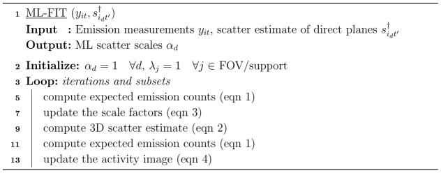
2.2. Iterative Algorithm for Scatter Scale Estimation: ML-FIT
Assuming Poisson statistics on the emission data yit, one can maximize the log-likelihood for emission tomography by updating the scatter scaling values αd as in (Defrise et al. 2014) and the tracer activity distribution λ as:
| (3) |
| (4) |
where (n) is the iteration index, 𝒪 is a 3D sinogram of all ones and cij = Σt citj is the TOF integrated sensitivity of voxel j to LOR i. After obtaining the scale factors αd, these factors are used to scale the scatter estimate of direct planes s† using (2), yielding what we will call the ML-SSS estimate in the following. Note that in our implementation (Algorithm 1) we chose to use the newly updated estimate of the ML scales (3), to recompute the expected emission measurements ȳ using (1), and to use it in (4). This alternating update implementation of (3) and (4) resulted in a (moderate) acceleration. Application of ordered subsets for further accelerating the two-step iterative algorithm is straightforward. The derivation of (3), the update equation of the ML scales, is given in Appendix A.
Algorithm 1.
Pseudo-code for ML-FIT
For technical reasons the ML-FIT algorithm is applied below using for s† either the single-scatter estimate (SSS), or the single-scatter estimate already scaled using “tail-fitting” (FT-SSS§). It is important to keep in mind that throughout the paper, the shape of the scatter estimates is (almost) the same for all methods, only the scale varies. One readily verifies from equations (1)–(4) that multiplying by some factors βd > 0 leaves the sequence of iterates unchanged provided the initial scales αd at iteration n = 0 are divided by the same factors βd. Thus using SSS or FT-SSS only amounts to changing the initialization and the converged solution is not modified.
2.3. Activity Reconstruction
Even though ML-FIT estimates the activity (eqn (4)), this activity image is disregarded. Following the estimation of the ML scatter scales, a “standard” (using 3 iteration of 24 subsets) MLEM activity distribution is reconstructed with the ML-SSS estimate. This allows us to compare MLEM activity images with different scatter estimates, all produced with the same reconstruction parameters, typically used in clinical setting. This also ensures that the activity images are not influenced by the data/image mashing or different number of iterations, the difference between the images is only caused by using a different scaling of the scatter estimate.
3. Experiment Design
In all the studies, the data were collected in 5D (radial position, azimuth angle, axial position, polar angle and TOF dimension) sinograms in the native Siemens format, and the e7tools (a collection of Siemens programs, callable from the command line in Microsoft Windows, dedicated to reconstruction from Siemens PET data, supporting CT-based attenuation correction) were applied to compute the expected scatter and randoms contributions to the TOF emission measurements in each bed position. Since the scatter contribution is estimated independently for each bed position, the scatter estimates of all bed positions were combined and, where the bed positions overlap, averaged (weighted by the axial sensitivity of the scanner) to give the expected scatter contribution across all direct planes. Furthermore, a virtual scanner was designed which enabled us to reconstruct the emission data acquired over all measured bed positions simultaneously.
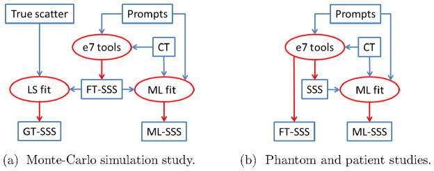
Figure 1 gives a flow chart of the experimental design. SSS denotes the (unscaled) single scatter estimate produced with the Siemens e7tools. FT-SSS denotes the (scaled) scatter estimate produced by “tail-fitting” the SSS to the sinogram data outside the patient support. ML-SSS denotes the (scaled) scatter estimated by computing the ML scale factor (simultaneously with estimating the activity).
Figure 1.
Flowcharts of the (FT-)SSS and ML-SSS estimates analyzed in this study. Note that the GT-SSS estimate is only available in the Monte-Carlo simulation study.
The experiments include the processing of a Monte-Carlo study, a phantom measurement and clinical scans. In the Monte-Carlo study, the true scatter contribution is known, and hence an optimal ground truth scaling can be calculated, yielding GT-SSS. In the Monte-Carlo study only the FT-SSS was available, therefore the ML-scaling was applied to rescale the FT-SSS. In the phantom and patient studies, we do not know the ground truth scale factor, the performance of the algorithm must be deduced from indirect evidence. In these studies, both the SSS and FT-SSS were available, and the ML-scaling was applied to rescale the SSS.
3.1. Monte-Carlo Simulation Study
A Monte-Carlo simulation study was conducted on a NEMA-like phantom with the Siemens Biograph mCT scanner specifications (Jakoby et al. 2011) to analyze the proposed ML scatter scaling. The Geant 4 toolkit (Allison et al. 2016) was used to simulate 511 keV photon transport in the phantom and detectors. In this simulation, multiple scattering, scatter in scintillator (broadening the point spread function) and depth of interaction (due to the scintillator attenuation) were simulated. However, the radionuclide and it’s positron range, acollinearity of the emitted photons, and scintillator light were not simulated. Energy and time of flight information were known exactly after the photon transport, however, both are blurred according to the scanner energy and TOF resolutions, respectively. A typical energy window of 435–650 keV is used for photons acceptance, inter-block scatter is rejected, and the photon arrival position is defined by the energy deposit. Furthermore, in this simulation, no random events were modeled. The obtained scatter fraction was 30.1% with a 6.25:1 ratio of single to multiple scattered events. The emission data were processed with Siemens’ e7tools, which provided the “tail-fitted” FT-SSS estimate. Since the simulation provides the actual single and multiple scatter components within the data, a least squares fit of the FT-SSS to the total (single plus multiple) simulated scatter estimates is considered as the ground truth (GT) and was compared to the estimated ML scatter scales. This GT scatter scale estimate was computed as the solution of the following linear system of equations:
| (5) |
where sSGL and sMLT are the single and multiple scatter components of the Monte-Carlo estimated emission data, respectively. Since (5) depends on the rebinning operation, a GT scatter scale is computed for each of the SSRB and MSRB rebinning operators. Appendix B gives the derivation of the GT scatter scale expression (5).
The ML scatter scales are computed jointly with an MLEM reconstruction of the activity using 10 iterations of 24 subsets. Initially, the ML scatter scales were computed with no radial mashing of the emission data and the activity distribution was reconstructed in a 2.04 mm × 2.04 mm × 2.03 mm voxel grid. In addition, the calculations were repeated with radial mashing factors of 2 and 4 (i.e. sub-sampling the radial sinogram index by a factor of 2 or 4, after summing sets of 2 or 4 adjacent radial bins). During these calculations, the same mashing factor was also applied to the voxel grid of the activity image in the transaxial plane. In all cases, the final (“standard”) MLEM reconstructions were computed with a voxel grid of 2.04 mm × 2.04 mm × 2.03 mm. Furthermore, the activity reconstruction was initialized with a uniform tracer distribution either in the support of the phantom or in the entire FOV of the scanner to study the stability of the ML scatter scales. The reference activity image (to which the reconstructions were compared) was obtained by applying MLEM to the true prompts (i.e. non scattered and non random events) in the emission data.
3.2. Phantom Data
A total activity of 74 MBq 18F-FDG was used to fill a custom-made phantom with a bladder insert. The activity in the bladder insert was 200 times higher than that in the background, to mimick a typical 68Ga-PSMA scan. The phantom was scanned on the Siemens Biograph mCT scanner across two bed positions. The ML scatter scales were subsequently obtained after 25 iterations of 24 subsets, with radial mashing factor of 4, and using the MSRB as the rebinning operator. Using a voxel grid of 8.14 mm × 8.14 mm × 2.03 mm the tracer distribution was reconstructed in a 100 × 100 × 172 volume. We report the results on “standard” MLEM activity reconstructions (using 3 iteration of 24 subsets and a voxel grid of 2.04 mm × 2.04 mm × 2.03 mm) with the SSS and the ML-SSS estimates used for scatter correction, respectively.
3.3. Patient Data
The ML scatter scaling was applied to 23 whole-body scans of patients (weight: 67.4 kg ± 14.4 kg) injected with 547 MBq ± 19 MBq of the 18F-FDG tracer. The local institutional review board approved this study and informed consent was obtained from all subjects. The emission data were acquired by the Siemens Biograph mCT scanner at New York Medical Center in 5–8 different bed positions, each scanned for 120 s per bed position. Similar to the phantom study, the ML scatter scales were obtained after 25 iterations of 24 subsets using the MSRB operator, applying a radial mashing factor of 4 to the TOF-PET emission data and using the virtual scanner to reconstruct the tracer distribution in a 8.14 mm × 8.14 mm × 2.03 mm voxel grid. The initial activity reconstruction was a uniform tracer distribution in the support of the patient (obtained by thresholding the CT attenuation image followed by a dilation operation to ensure that the body contour was not too narrow). As before, we report the results on “standard” MLEM activity reconstructions (using 3 iterations of 24 subsets and a voxel grid of 4.07 mm × 4.07 mm × 2.03 mm) with the SSS, FT-SSS and the ML-SSS estimates used for scatter correction, respectively.
4. Results
4.1. Monte-Carlo Simulation Study
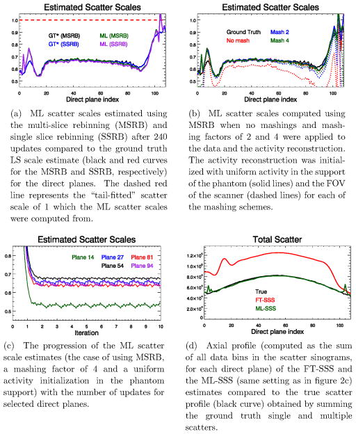
Figure 2a shows the final scatter scales estimated after 240 updates. The ground truth LS fit and the ML-SSS were computed using the (already scaled) FT-SSS, and hence the results suggest that the “tail-fitting” of the SSS estimate has overestimated the scatter in the emission data by roughly a factor of 2. Figure 2d plots the corresponding scatter profiles (computed as the sum of all data bins in the scatter sinograms, for each direct plane) of the true total scatter (single and multiple) and of the FT-SSS and ML-SSS scatter estimates.
Figure 2.
Results of the Monte-Carlo simulation study, (a): scatter scales, (b): effect of mashing and activity initializations, (c): progression of the scales, (d): axial scatter profiles.
Figure 2b shows the ML scatter scales estimated using the different mashing and activity initialization schemes. The ML-procedure tends to produce a more accurate estimate of the scatter scale (and hence a better ML-SSS) when the emission data are mashed and subsequently reconstructed in a coarser (transaxial) voxel grid. In this study, the initialization of the activity reconstruction seems to have a minimal effect on the estimated ML scales except for the case where no mashing was applied.
Figure 2c shows the computed ML scale values as a function of the iterations for 5 direct planes. For all planes the ML scatter scale reaches a plateau already after the first iteration (24 updates) and remains stable when applying more iterations of the joint ML scatter scale and activity reconstructions algorithm. It should be noted that in the Monte-Carlo simulation random coincidence events were not modeled.
Figure 3 shows the ground truth (GT) MLEM activity reconstruction (obtained by reconstructing only the true prompts in the TOF-PET emission data) as well as the difference of activity reconstructions of MLEM compared to the ground truth when the FT-SSS and the ML-SSS estimates were used for scatter correction of the TOF-PET emission data. Because the FT-SSS estimate over-estimates the scatter within the emission data (as shown in figure 2), using FT-SSS for scatter correction underestimates the total tracer activity of the MLEM reconstruction by 17.4%. In contrast, when the ML-SSS estimate was used for scatter correction, the total tracer activity of the MLEM reconstruction was slightly over-estimated by 0.5%. Furthermore, a different bias structure is observed when comparing the difference images of MLEM with the FT-SSS and the ML-SSS estimates. Although the MLEM activity reconstruction with the ML-SSS estimate has produced a slightly different noise profile compared to the ground truth, it seems to be free of any systematic bias.
Figure 3.
Ground truth activity reconstruction (left) obtained by reconstructing the true prompts and difference images of MLEM activity reconstructions (right) compared to the ground truth. The difference images were obtained by using the FT-SSS (top) and the ML-SSS (bottom) estimates for scatter correction. (For comments on the black arrow in the figure, see the supplementary material.)
4.2. Phantom Data
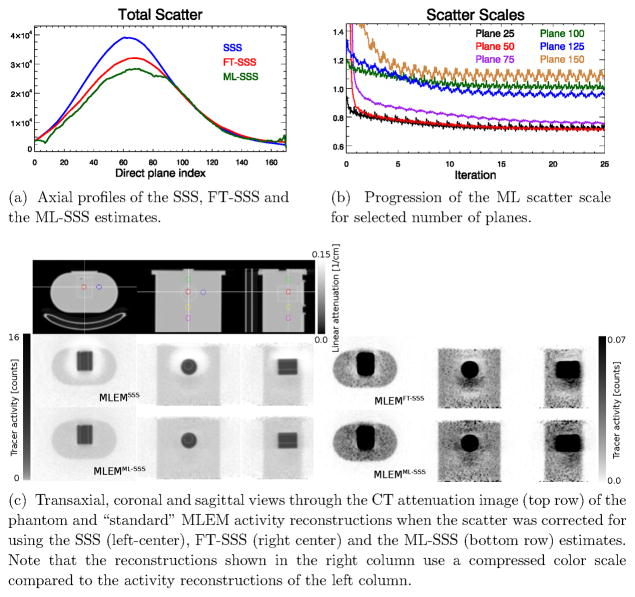
Figures 4c shows MLEM reconstructions with the SSS, FT-SSS and the ML-SSS estimates of the expected scatter in the emission data. The “halo” artifacts are no longer present in the tracer distribution reconstruction using the ML-SSS estimate. In order to analyze the tracer distribution reconstructions, a hot to background uptake ratio was computed from spherical regions of interest (ROIs) of 28.5 mm diameters depicted in the CT attenuation image (figure 4c-top). Table 1 reports, for the three activity reconstructions, the ratio between the uptake in the hot region (H) and in different cold background regions (Ck, k = 1, 2, 3, 4). Note that this ratio is very sensitive to a possible bias due to inaccurate scatter background. The uptake ratios demonstrate that correction for scatter using the ML-SSS estimate provide reconstructions that are quantitatively more accurate compared to the reconstructions using either the SSS or the FT-SSS estimates.
Figure 4.
Results of the phantom study.
Table 1.
Tracer uptake ratios computed using the spherical regions of interest (ROIs) shown in figure 4c. The true uptake ratio is 200.
| H/C1 | H/C2 | H/C3 | H/C4 | |
|---|---|---|---|---|
| SSS | 6.7×10⁷ | 84.5 | 2.6×10⁴ | 265.8 |
| FT-SSS | 415.0 | 84.4 | 325.4 | 501.9 |
| ML-SSS | 120.4 | 119.4 | 159.1 | 199.5 |
Figure 4 also shows the total scatter contributions of the direct planes (4a) and the estimated ML scatter scales for a selected number of direct planes (4b), respectively.
4.3. Patient Data
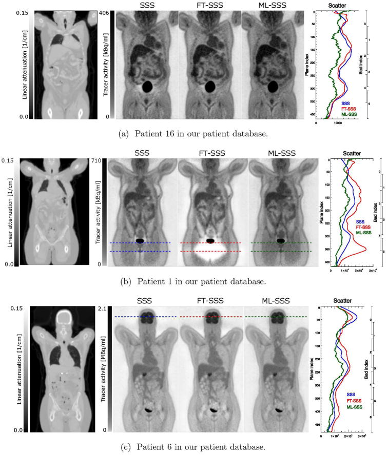
When computing the ML scatter scaling values for the patient data, a radial mashing factor of 4 was used during reconstructions and the activity reconstruction was initialized with a uniform tracer distribution in the support of the patient. As for the phantom study, the ML scaling was applied to the SSS estimate (rather than the FT-SSS estimate, as in the case of the Monte-Carlo study). Although the results vary over the different planes, FT-SSS tends to produce scale factors larger than 1, whereas ML-SSS typically produces scale factors less than 1 (0.831, average across all patients and 2D planes). This agrees with the Monte-Carlo simulation experiment.
Figure 5 shows three MLEM reconstructions, two of which are of the more extreme cases where the SSS (figure 5a) and the FT-SSS (figure 5b) have over-estimated the scatter contribution, resulting in a local under-estimation of the tracer distribution close to the bladder. The “halo” artifacts are no longer present in the tracer distribution reconstruction using the ML-SSS estimate. For approximately 50% of our patient database visual inspection showed no significant change using the ML-SSS estimate, the FT-SSS or the SSS. Nevertheless, compared to the activity reconstructions with the SSS estimate, the FT-SSS and the ML-SSS reconstructions on average changed the total amount of tracer activities over all our patient database by −2.8% and 12.2%, respectively.
Figure 5.
“Standard” (using 3 iteration of 24 subsets and a voxel grid of 4.07 mm × 4.07 mm × 2.03 mm) MLEM activity reconstructions of three different patient datasets. For each patient the activity reconstruction using the SSS (left), the FT-SSS (center), and the ML-SSS (right) estimates are shown together with the total scatter in the direct planes.
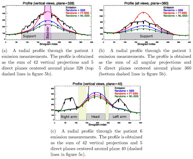
Figure 6 shows radial profiles through the TOF-PET emission data for planes shown by the dashed lines for two of the patient reconstructions shown in figure 5. In some cases the FT-SSS scatter estimate exceeded the measured emission counts (either close to the bladder as shown in figure 6a or between the head and the arms of the patient as shown in figure 6c), whereas the ML-SSS estimate was below or equal to the measured counts. This provides evidence that in these cases FT-SSS overestimated the scatter contribution and that the ML-SSS estimate was more accurate. Although visual inspection shows no obvious signs of artifacts in the patient reconstruction shown in figure 5c, close inspections around the head of the patient reveals signs of the “halo” artifacts which are more pronounced in the reconstructions of patients 16 and 1. However, the brain region seems to be less affected by this “halo” effect as reconstructions of high count regions in the emission data are expected to be less sensitive to these inconsistencies.
Figure 6.
Radial profiles through the emission measurements and the 3 scatter estimates (SSS, FT-SSS and ML-SSS).
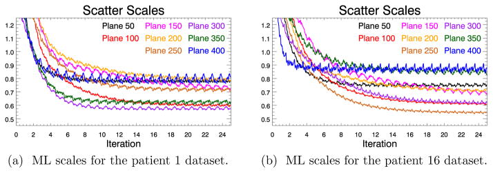
Figure 7 shows the ML scatter scales computed as a function of the iteration number for a selected number of direct planes for two of our patient datasets. It is observed that for most of the direct planes a larger number of iterations is needed to reach a plateau than for the Monte-Carlo simulation, which could be the effect of the additional background contribution of the randoms in the patient emission data. Apart from the ML scatter scales close to the patient chest which seem to decrease with more iterations, the ML scales appear to be stable with more iterations of the algorithm. A possible explanation for this effect could be the respiratory motion which can cause inconsistencies in the emission data.
Figure 7.
Progression of the ML scatter scales with increasing number of updates for selected direct planes. See figure 5 for the relation between plane numbers and anatomy.
5. Discussion
The use of the entire emission sinogram as opposed to using only the “scatter tails” of the emission sinogram for the estimation of the scatter scale has been previously investigated by Thielemans et al. (2007) and Panin (2012). In this contribution, we extended a recently developed ML scatter scale estimation algorithm (Defrise et al. 2014; Salvo et al. 2015) to account for a plane dependent scatter scale. Since the model-based simulated single scatter (SSS) estimate was only computed for direct planes, a scaling factor was introduced for each of the direct planes and after the application of the scales a fully 3D scatter estimate was obtained by transpose-rebinning the ML-SSS estimate.
The algorithm is computationally expensive. Therefore, the TOF-PET emission data and the reconstruction volume grid were mashed to accelerate the algorithm, which also helped stabilize the ML scales, in agreement with the findings of Defrise et al. (2014). Nevertheless, the plane-dependent ML scatter scale computation and the subsequent update of the 3D scatter estimate increased the reconstruction processing time by 80% (calculated for the MSRB with a mashing factor of 4 and in one bed position). We found that the ML scales were also more reliable when the activity reconstruction was restricted to the phantom/patient support (fig 2b). In this study the TOF multi-slice rebinning (MSRB) operator was used as the rebinning operator of choice. However, very similar results were obtained when the TOF single-slice rebinning (SSRB) operator was used instead.
A relatively fast convergence of the ML scatter scales was observed for the simulated data. However, when the ML scatter scales were computed for the patient dataset more updates of the joint ML algorithm were needed. This could in part be explained by the added background contribution of the randoms, which were not modelled in the simulation experiment, as well as a lower scatter fraction for the patient emission data. Direct validation of the estimated ML scatter scales was made possible in the simulation as the total contributions of multiple and single scatters were known. The estimated ML scatter scales agreed well with the “best possible scale”, which was computed using a least squares fit to the known scatter distribution. The elimination of the “halo” artifact typically observed near high focal uptake regions as well as the analysis of emission and scatter profiles provided indirect evidence for the accuracy of the ML scatter scales in the patient studies.
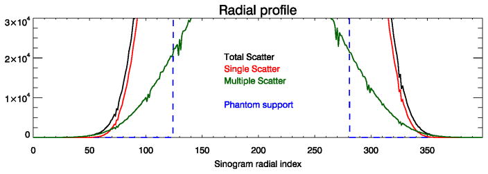
The Monte-Carlo simulation results of the NEMA-like phantom demonstrated how inaccuracies in scatter scaling can cause both a global and a local bias effect on the reconstruction of the PET tracer distribution. When the FT-SSS estimate was used for scatter correction, the total amount of tracer activity was under-estimated by 17%. When the proposed ML scatter scaling method was used to modify the scales of the FT-SSS estimate, the global error was reduced to less than 1%. As a result, the comparison with the gold-standard MLEM reconstruction showed no significant sign of the locally structured bias observed with the FT-SSS scatter estimate. We believe that inaccuracies in determining the “scatter-tails” will cause in most cases an over-estimation of scatter by FT-SSS. Figure 8 shows the true radial profiles of the total, single and multiple scatters in the simulated emission data. The true single scatter is seen to be an accurate estimate of the total amount of scatter closer to the phantom support. However, selection of data bins in the vicinity of the support as “scatter-tails” are typically avoided in practice to limit the number of true coincidences in the “scatter-tails” which could occur due to e.g. patient motion. Farther away from the patient support single scatter becomes a less accurate predictor of the total scatter due to the more dominating effect of multiple scatters. In both of these cases (“scatter-tails” selected either too close or too far from the support) and with an accurate estimate of the single scatter shape, FT-SSS will over-estimate the scatter contribution.
Figure 8.
Radial profiles of the true scatter estimates of the Monte-Carlo simulation study.
In the phantom study, the ML-SSS not only eliminated reconstruction artifacts, it also improved the quantitative accuracy of the reconstruction. Furthermore, we found that the typical “halo” artifacts caused by an inaccurate scatter estimate were also removed from the patient image reconstructions by using the ML-SSS estimates. Similar to the simulation study, the total amount of reconstructed tracer uptake increased, for the patient reconstructions by a factor of 12%. As illustrated in figure 5, the differences between the SSS, FT-SSS and ML-SSS estimates depend on the patient and on the position in the patient. Therefore, the scatter scaling algorithm is expected to affect not only the quantification of a single study, but also the evolution of the estimated activity over time in dynamic studies or in a studies done for patient follow up. Further studies are warranted to analyze and verify the applicability of the proposed ML scaling method to the estimation of the scatter scaling factors for other radioactive tracers.
We have previously observed that MLEM and MLAA algorithms (Rezaei et al. 2012) reconstruct similar activity images when the data are consistent, but they tend to converge to different solutions in the presence of data inconsistencies. Hence, we believe that the difference between MLEM and MLAA activity reconstructions is an indicator of data consistency. A study of MLEM and MLAA activity images using the different scatter estimates is provided in the supplementary material.
6. Conclusion
An extension of the ML scatter scaling is proposed and validated on simulated data as well as clinical patient scans. The ML scatter estimate provides a more accurate estimate of the scatter scale in the emission data by using data from the entire emission measurements as opposed to the “scatter tails” as is often used in practice. The activity reconstructions using the ML-SSS estimate seem to be free of scatter over-estimation artifacts.
Supplementary Material
Acknowledgments
The authors would like to thank Dr. Maurizio Conti and Dr. Harshali Bal from Siemens Medical Solutions, MI, Knoxville, USA for providing the phantom measurements. This work was supported in part by the Research Foundation Flanders (FWO), project G.0275.14N and by the Center for Advanced Imaging Innovation and Research, a National Institute for Biomedical Imaging and Bioengineering Biomedical Technology Resource Center (NIH P41 EB017183).
Appendix A
Extending the ML scatter scaling of (Defrise et al. 2014) to account for an independent scatter scale per direct plane, the multiplicative update factor during the iterations becomes:
| (6) |
The update of each direct plane is then normalized using:
| (7) |
Combining (6) and (7) gives the update expression (3) for the ML scatter scales.
Appendix B
The ground truth plane-dependent scatter scales are obtained by minimizing the quadratic differences of the scatter estimate sit computed from (2) and the true estimate of scatter ŝ. Setting the derivative of this quadratic cost function with respect to the scatter scales αd to zero we have:
| (8) |
| (9) |
re-arranging gives (5).
Equation (5) defines a system of linear equations of the form Aα = b which we solve to obtain the least squares solution as α̂ = [AT A]−1ATb. E.g. in the case of a single bed scan on the mCT scanner, A is a matrix of [109, 109], α̂ is the least squares ground truth scales of size [109] and b is also a vector of length [109] which is computed from the known scatter estimate.
Appendix C
Although the SSRB algorithm was used only in the Monte-Carlo simulation study for estimating the plane-dependent ML scatter scales, the MSRB algorithm was used in all studies. The MSRB rebinning algorithm was proposed by (Lewitt et al. 1994) to attenuate the artifacts observed with SSRB at increasing distances from the scanner axis. MSRB estimates a 2D data bin (d, t′) as an average of all 3D data bins (i, t) which intersect the 2D data bin. This procedure is followed by an axial deconvolution step to reduce the loss of resolution in the axial direction. Our TOF implementation of the MSRB omits the axial deblurring since this is not expected to be a limitation in view of the smoothness of the scatter background.
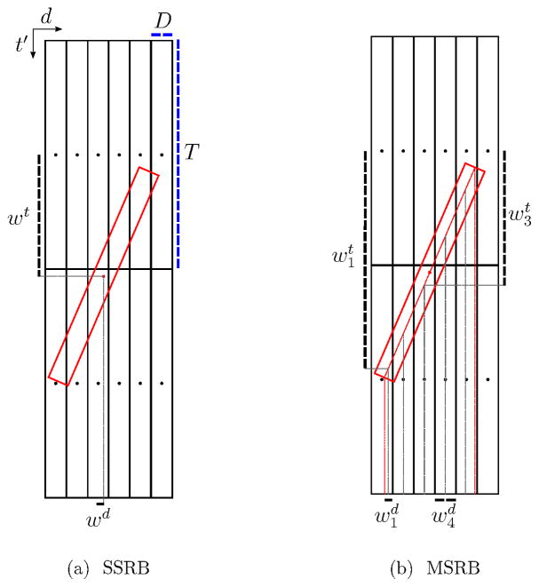
Figure 9 shows schematic of multiple 2D data bins, from which an oblique data bin (show in red) is computed, using the SSRB and MSRB algorithms. Given v(d,t′), the value of the 2D data bin (d, t′), for all direct data bins, the SSRB and the MSRB algorithms compute the value of the oblique data bin as:
| (SSRB) |
| (MSRB) |
where D and T are the widths of the data bin in the planar and TOF directions and δ is the Kronecker delta function. For the SSRB expression, wd and wt denote the distances between the center of the considered oblique 3D-bin and the direct 2D-bin (3, 1) in the detector and TOF directions, respectively. For MSRB, the definitions are a bit more complicated. The centerline of the oblique 3D-bin is computed, and for each detector index i, the part of that centerline overlapping with crystals i is considered. The vertical distance of the center of that centerline part to the center of crystal (d, 1) is denoted as ). In addition, a weight is computed: this weight equals unity if the 3D-bin traverses the 2D-bin i, but is less than unity if the 3D-bin overlaps with the 2D-bin without completely traversing it.
Figure 9.
Schematic of 2D data bins which the value of an oblique data bin (shown in red) is computed from using SSRB and MSRB algorithms. In this example, the crystals are numbered from left to right (1–6), the TOF-bins from top to bottom (1–2).
Footnotes
For a single bed-position and for the Siemens Biograph mCT scanner the TOF-PET emission data are stored in a total of 621 sinogram planes which 109 are direct planes (Jakoby et al. 2011). In the case of multiple bed acquisitions the number of direct planes increases by the total number of direct planes covered by the acquisitions of all bed positions.
To avoid confusion with the acronym used for time of flight we use FT for “tail-fitted”.
References
- Adam LE, Karp JS, Freifelder R. Energy-Based Scatter Correction for 3-D PET Scanners Using Nal(TI) Detectors. ENG In: IEEE transactions on medical imaging. 2000;19(5):513–521. doi: 10.1109/42.870261. [DOI] [PubMed] [Google Scholar]
- Allison J, et al. Recent Developments in Geant4. Nuclear Instruments and Methods in Physics Research Section A: Accelerators, Spectrometers, Detectors and Associated Equipment. 2016;835:186–225. [Google Scholar]
- Bailey DL, Meikle SR. A Convolution-Subtraction Scatter Correction Method for 3D PET”. ENG. Physics in Medicine and Biology. 1994;39(3):411–424. doi: 10.1088/0031-9155/39/3/009. [DOI] [PubMed] [Google Scholar]
- Bendriem B, Trebossen R, Frouin V, Syrota A. A PET Scatter Correction Using Simultaneous Acquisitions with Low and High Lower Energy Thresholds. Nuclear Science Symposium and Medical Imaging Conference, 1993., 1993 IEEE Conference Record; 1993. pp. 1779–1783. [Google Scholar]
- Casey ME, Hoffman EJ. Quantitation in Positron Emission Computed Tomography: 7. A Technique to Reduce Noise in Accidental Coincidence Measurements and Coincidence Efficiency Calibration”. eng. Journal of Computer Assisted Tomography. 1986;10(5):845–850. [PubMed] [Google Scholar]
- Defrise M, Salvo K, Rezaei A, Nuyts J, Panin VY, Casey ME. ML Estimation of the Scatter Scaling in TOF PET. 2014 IEEE Nucl Sci Symp Med Imaging Conf (2014 NSS/MIC) 2014 [Google Scholar]
- Grootoonk S, Spinks TJ, Sashin D, Spyrou NM, Jones T. Correction for Scatter in 3D Brain PET Using a Dual Energy Window Method”. ENG. Physics in Medicine and Biology. 1996;41(12):2757–2774. doi: 10.1088/0031-9155/41/12/013. [DOI] [PubMed] [Google Scholar]
- Jakoby BW, Bercier Y, Conti M, Casey ME, Bendriem B, Townsend DW. Physical and Clinical Performance of the mCT Time-of-Flight PET/CT Scanner. Phys Med Biol. 2011;56(8):2375–89. doi: 10.1088/0031-9155/56/8/004. [DOI] [PubMed] [Google Scholar]
- Lewitt RM, Muehllehner G, Karp JS. Three-Dimensional Image Reconstruction for PET by Multi-Slice Rebinning and Axial Image Filtering”. en. Physics in Medicine and Biology. 1994;39(3):321. doi: 10.1088/0031-9155/39/3/002. [DOI] [PubMed] [Google Scholar]
- Oliver JF, Rafecas M. Modelling Random Coincidences in Positron Emission Tomography by Using Singles and Prompts: A Comparison Study. PLOS ONE. 2016;11(9):e0162096. doi: 10.1371/journal.pone.0162096. [DOI] [PMC free article] [PubMed] [Google Scholar]
- Ollinger JM. Model-Based Scatter Correction for Fully 3D PET”. ENG. Physics in Medicine and Biology. 1996;41(1):153–176. doi: 10.1088/0031-9155/41/1/012. [DOI] [PubMed] [Google Scholar]
- Panin VY. Scatter Estimation Scaling with All Count Use by Employing Discrete Data Consistency Conditions. 2012 IEEE Nuclear Science Symposium and Medical Imaging Conference (NSS/MIC); 2012. pp. 2998–3004. [Google Scholar]
- Rezaei A, Defrise M, Bal G, Michel C, Conti M, Watson C, Nuyts J. Simultaneous Reconstruction of Activity and Attenuation in Time-of-Flight PET. IEEE Trans Med Imaging. 2012;31(12):2224–33. doi: 10.1109/TMI.2012.2212719. [DOI] [PubMed] [Google Scholar]
- Salvo K, Panin VY, Rothfuss H, Defrise M. ML Estimation of the Scatter Scaling in TOF PET. 2015 Fully Three-Dimensional Image Reconstruction in Radiology and Nuclear Medicine Proceedings 2015 [Google Scholar]
- Sossi V, Stazyk MW, Kinahan PE, Ruth TJ. The Performance of the Single-Slice Rebinning Technique for Imaging the Human Striatum as Evaluated Bp Phantom Studies”. en. Physics in Medicine and Biology. 1994;39(3):369. doi: 10.1088/0031-9155/39/3/005. [DOI] [PubMed] [Google Scholar]
- Thielemans K, Manjeshwar RM, Tsoumpas C, Jansen FP. A New Algorithm for Scaling of PET Scatter Estimates Using All Coincidence Events. 2007 IEEE Nuclear Science Symposium Conference Record. 2007;5:3586–3590. [Google Scholar]
- Watson CC. New, Faster, Image-Based Scatter Correction for 3D PET. IEEE Transactions on Nuclear Science. 2000;47(4):1587–1594. [Google Scholar]
- Watson CC. Extension of Single Scatter Simulation to Scatter Correction of Time-of-Flight PET. IEEE Trans Nucl Sci. 2007;54(5):1679–1686. [Google Scholar]
Associated Data
This section collects any data citations, data availability statements, or supplementary materials included in this article.


