Metabolomic Analysis and Visualization Engine for LC–MS Data

Abstract

Metabolomic analysis by liquid chromatography–high-resolution mass spectrometry results in data sets with thousands of features arising from metabolites, fragments, isotopes, and adducts. Here we describe a software package, Metabolomic Analysis and Visualization ENgine (MAVEN), designed for efficient interactive analysis of LC–MS data, including in the presence of isotope labeling. The software contains tools for all aspects of the data analysis process, from feature extraction to pathway-based graphical data display. To facilitate data validation, a machine learning algorithm automatically assesses peak quality. Users interact with raw data primarily in the form of extracted ion chromatograms, which are displayed with overlaid circles indicating peak quality, and bar graphs of peak intensities for both unlabeled and isotope-labeled metabolite forms. Click-based navigation leads to additional information, such as raw data for specific isotopic forms or for metabolites changing significantly between conditions. Fast data processing algorithms result in nearly delay-free browsing. Drop-down menus provide tools for the overlay of data onto pathway maps. These tools enable animating series of pathway graphs, e.g., to show propagation of labeled forms through a metabolic network. MAVEN is released under an open source license at http://maven.princeton.edu.

LC–MS-based metabolomics is an increasingly important contributor to cell biology,¹ pathophysiology,^{2, 3} and biomarker identification.^{4, 5} Despite steady improvements in LC–MS methods and data analysis software, manual review of raw data continues to be both necessary and time-consuming.⁶ This is particularly true for full scan LC–MS analysis, where compound identification relies on exact mass and retention time. Several factors contribute to the burden of data validation: run-to-run retention time variation, poor signal-to-noise for low abundance metabolites, the presence of numerous peaks from isotopes, adducts, and in-source degradation products, and the presence of unexpected metabolites and contaminants.

A typical LC–electrospray ionization-MS experiment yields several thousand ion peaks, of which 100–200 correspond to [M + H]⁺ or [M − H]⁻ peaks of identified metabolites.⁷ In experiments involving isotope labeling, the number of peaks increases several-fold, further complicating analysis. To convert the raw data into a validated table of compound-specific peak intensities, an analyst may spend tens or hundreds of hours reviewing extracted ion chromatograms, comparing peaks to those of authenticated standards, and searching databases for potential matches to unidentified peaks.

To expedite this process, software is critical. A number of high-quality open source software packages have been developed.^8–13 For example, XCMS enables feature extraction, peak alignment, and identification of peaks that vary significantly between a set of control and experimental samples.⁸ Review of the peaks of interest is then conducted by the analyst using other software (e.g., that supplied by the instrument vendor). While this process has proven effective for discovering metabolites that respond strongly to biological perturbations,^14–16 the need to separately review raw data and manually re-enter any peaks misannotated by automated processing methods is tedious when the goal is metabolome-wide quantitation.^17–19Accordingly, it would be useful to have software that couples automated feature detection and peak alignment with online data visualization and annotation. To this end, we have developed a Metabolomics Analysis and Visualization Engine (MAVEN). In addition to the key LC–MS data processing functionalities, MAVEN provides nearly instantaneous querying of raw data, machine learning-based assessment of peak quality, graphical presentation of raw data with visual cues that expedite manual review, automated analysis of isotope-labeled forms, and graphical mapping of data onto metabolic pathways. Navigation by mouse allows the user to access screens focusing on raw data, adducts, isotopic variants, and pathways in a seamless manner, with the ability to manually correct misannotations throughout. The end result is a more rapid and reliable attainment of validated data appropriate for biological analysis and quantitative modeling.

EXPERIMENTAL METHODS

Biological Reagents and Cell Culture

Human foreskin fibroblasts were cultured in Dulbecco’s Modified Eagle’s Medium (DMEM) with 10% fetal bovine serum and 4.5 g/L of glucose. The fibroblasts were grown to confluence in 60 mm dishes resulting in ~1.5 × 10⁶ cells per plate. The cells were maintained at confluence for 4 days prior to infection and then serum starved for 24 h. Following serum starvation, the cells were infected with human cytomegalovirus (AD169 strain) at a multiplicity of infection of three plaque-forming units per cell or mock treated with virus-free inoculum. After a 1 h absorption period, the inoculum was aspirated and fresh and serum-free DMEM was added. The medium was changed on the plates at 24 h postinfection and at 46 h postinfection to fresh DMEM. At 48 h postinfection, DMEM containing uniformly ¹³C-labeled glucose was added to the plates.

Metabolite Extraction and LC–MS

At various time points following addition of labeled DMEM, metabolites were harvested as previously described.²⁰ After drying the samples, the metabolites extracted from the infected plates were dissolved in 600 µL of HPLC-grade water, while metabolites from mock-treated plates were dissolved in 300 µL. This 2-fold difference in volume accounts for the ~2-fold increase in volume of the fibroblasts during human cytomegalovirus infection. Volumes of 10 µL of each metabolite extract were analyzed via reversephase ion-pairing chromatography coupled to a stand-alone orbitrap mass spectrometer. The mass spectrometer scan rate was set to 1 Hz and resolving power to 100 000, scanning m/z 85–1000 in the negative ion mode. All other parameters are as in Lu et al.²¹ The LC gradient was 0 min, 0% B; 2.5 min, 0% B; 5 min, 20% B; 7.5 min, 20% B; 13 min, 55% B; 15.5 min, 95% B; 18.5 min, 95% B; 19 min, 0% B; 25 min, 0% B. Solvent A is 97:3 water–methanol with 10 mM tributylamine and 15 mM acetic acid; solvent B is methanol. The flow rate was 200 µL/min on a Synergy Hydro-RP column (100 mm × 2 mm, 2.5 µm particle size, Phenomenex, Torrance, CA).

RESULTS AND DISCUSSION

Overview of Software

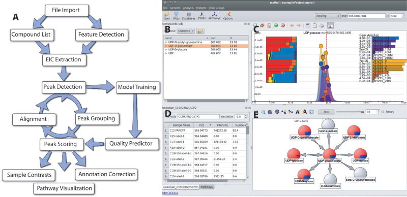
Figure 1A outlines the basic MAVEN workflow. Unlike fully automated metabolomics packages, MAVEN is an interactive analysis environment, and accordingly there is no fixed pipeline. Data is loaded as centroided mzXML or mzData files (~20 megabytes each; ~100 files can be opened simultaneously on a midrange desktop). The user decides whether to interactively examine the data on a compound-by-compound basis or to have MAVEN detect mass slices and pull out all peaks. In the first case, there is the option to click on compounds in a pre-entered list or to type a compound name, formula, or m/z range into a dialogue box. In the latter case, a feature detection algorithm (described below) identifies every m/z for which a peak exists in any sample. Once a target m/z is selected, MAVEN then extracts the associated ion-specific chromatogram (EIC) for all samples, detects peaks, groups peaks across samples, scores their quality, and displays the resulting raw data and analyses for visual examination. On a modern desktop processor, the program is capable of preforming these steps rapidly (see Supplementary Table 1 in the Supporting Information). For example, when processing 16 samples from a recent experiment involving virally infected fibroblasts and ¹³C-glucose labeling, MAVEN detected ~5600 mass slices, pulled out ~90 000 EICs, detected and quality scored ~137 000 peaks, and grouped them into ~5700 groups in ~20 s. Further workup of the data is achieved using a set of interactive tools. When focused on a predetermined list of known compounds, users will typically scroll down the list, checking MAVEN’s peak selection, correcting any misannotated peaks, and exporting (via a single mouse click) the validated peak intensities to a spreadsheet. MAVEN will detect automatically any associated isotopic peaks, score their quality, and export also their intensities. In addition, the software contains tools for projecting data onto metabolic pathways (e.g., from KEGG or Ecocyc). When untargeted analyses are conducted, it is common to focus on peaks that differ across two biological conditions. In addition to reporting a list of all peaks meeting a certain p-value threshold, MAVEN can display a scatter plot of peak intensities in condition 1 versus in condition 2, with the size of dots in the plot corresponding to the magnitude of the between-condition difference and their color corresponding to the statistical significance of the difference. Clicking on dots automatically pulls out the associated EIC. In addition, the software will highlight dots on the scatter plot that are likely to be isotopes, adducts, and fragments of the selected peak based on chromatographic coelution, peak shape similarity, and correlation in peak intensities across samples.

Figure 1.

Software overview. (A) General workflow. The program will automatically extract ion-specific chromatograms (EICs), assign peak quality scores, align peaks, and visually display data. The program is designed to allow an analyst to intervene at all stages. This facilitates correct annotation of detected features to compounds. (B–D) Screenshot of user interface. Shown is one common screen layout using UDP-glucose as a model compound. Subcomponents are (B) table of compounds with known retention times, (C) EIC centered on m/z and retention time of UDP-glucose, (D) table of isotope-labeled forms of UDP-glucose, and (E) reactions of UDP-glucose. All aspects are interlinked to enable efficient mouse-driven navigation through complex metabolomics data. For example, clicking on a different compound from the list in part B would automatically update screens C–E.

From Raw Data to Aligned Peaks

The MAVEN workflow follows similar steps to XCMS and mzMine: mass slice detection, extraction of ion-specific chromatograms (EICs), baseline detection for each EIC, data smoothing, peak picking and grouping, and retention time alignment.^{22, 23} At several steps, MAVEN includes algorithmic modifications that enable interactive data analysis without processing delays. The remainder of this section provides information on these algorithmic aspects; readers interested primarily in software capabilities may skip to the next section.

MAVEN’s feature detection algorithm works by sequentially evaluating every mass spectrum (scan) in every sample, searching for consecutive scans containing the same m/z value within the mass error of the instrument. The occurrence of detectable signal at the same m/z in consecutive scans is a minimal requirement for a peak; nevertheless, it is a sufficiently stringent requirement to eliminate most artifacts, e.g., from electronic noise. The resulting list of m/z values and corresponding retention times are recorded as mass-retention time slices.

For each mass-retention time slice, the EIC is extracted for all loaded samples. The speed of EIC extraction is critical to overall software performance. To this end, we employ a simple but rapid algorithm involving a binary search of each mass spectrum within the relevant retention time window for signal in the mass range of interest. A binary search takes advantage of m/z-ion intensity signal being ordered within each mass spectrum by m/z. It first inspects the middle m/z of the mass spectrum: if the middle m/z falls within the specified mass range of the EIC, then the sought m/z-intensity value pair has been found; otherwise, the upper half or lower half of the list is chosen for further searching based on whether the specified m/z is greater than or less than the middle m/z. The process is then repeated until an m/z that falls within the specified mass range is found. Signal extraction by binary search is sufficiently fast that there is generally no perceptible delay between entering a compound query and visualizing the EIC.

To enable reliable peak detection and quantitation for each EIC, MAVEN first calculates the EIC baseline. To remove nonbaseline points, the 20% of data points with the highest intensities are discarded. The remaining data is then Gaussian smoothed (i.e., the intensity of each point is replaced with a centered-weighted average of the surrounding points). The width of the Gaussian smoothing for baseline calculation is a user-specific parameter. An appropriate width for baseline detection is a typical peak width, e.g., 20 scans at 1 Hz. The median of the resulting set of smoothed intensities is taken as the baseline. Once the baseline is determined, the raw EIC (including also the top 20% of data points) is Gaussian smoothed with a smaller width, typically 5 scans. Peak centers are points in the smoothed EIC that are higher than their neighbors on both sides. Front and rear peak boundaries are where the derivative changes sign or intensity falls below baseline. Peak centers and boundaries enable calculation of peak height and area, respectively. Area calculations do not include any portions of the peak that fall below the EIC baseline. Once quantified, peaks are then quality-scored using a machine-learning approach, which is described in the following section.

The next step is to group peaks across samples. The grouping algorithm begins by computing a summed EIC: adding up the EICs for a given m/z across all samples. Peaks are detected in the summed EIC as above. The peaks in the summed EIC define “groups,” to which peaks in the individual EICs are assigned based on overlap in retention time. In contrast to algorithms that involve combinatorial grouping of individual peaks, where computational time may scale as the factorial of the number of samples, computational time of the MAVEN grouping algorithm scales linearly with the number of samples. Thus, speed is enhanced, especially for large sample sets.

Retention time alignment aims to shift chromatograms so that peaks in the same group coelute. This facilitates visualization and also can identify grouping errors: peaks that fail to coelute after retention time alignment. MAVEN uses groups that contain multiple peaks with high quality scores for chromatogram alignment. The alignment process involves iterative fitting with a global third degree polynomial. For each group, the median retention time of the peak center is determined. The retention time in each chromatogram is then shifted via the third-degree polynomial that leads to the best agreement between the shifted chromatogram peak centers and the median peak centers. This process is then repeated iteratively until convergence, typically three times. After chromatogram alignment, the analyst can choose to regroup peaks. This will not alter grouping of the high-quality peaks used for chromatogram alignment but can improve accuracy in the grouping of lower quality peaks. An example of three iterations of alignment for peaks in the folate (pteroylglutamic acid) EIC is shown in Supplementary Figure 1 in the Supporting Information. In general, chromatogram alignment works well for minor deviations in retention time (e.g., typical intraday variation), but repeated attempts at alignment with different user parameters may be required to correctly align chromatograms with more substantive retention time alterations (e.g., due to changes in column performance). Particularly important user-specified parameters relate to the minimum intensity of peaks selected to create the alignment and the retention time window across which peaks are grouped together (for full list of parameters, see the legend of Supplementary Figure 1 in the Supporting Information).

Automated Scoring of Peak Quality

While parameters like signal-to-noise are reported by many software packages as metrics of peak quality, no single parameter comes close to matching the judgment of a skilled analyst. We aimed to develop an algorithm for peak quality scoring that would do so. The resulting peak quality scores would enable identification of high-quality peaks for chromatogram alignment (see above), of borderline quality peaks that merit analyst review, and of low-quality peaks that can safely be ignored.

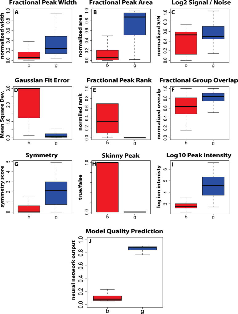
Our approach involved training a machine-learning algorithm using a set of LC–MS peaks manually annotated by an expert analyst as “good” or “bad.” The machine-learning algorithm, based on a neural network, integrates information from nine metrics of peak quality (Supplementary Figure 2 in the Supporting Information) in an effort to match the manual annotation. The neural network scores peaks on a continuous scale from 0 (bad) to 1 (good), with borderline quality peaks receiving intermediate scores.

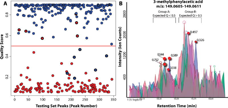
Each of the nine peak quality metrics is individually somewhat effective at distinguishing “good” and “bad” peaks (Figure 2A–J). The neural network substantially out-performs any individual metric (Figure 2K). A dichotomous split at a neural network score of 0.5 results in agreement between the computational and manual analysis for >95% of the peaks. All instances of disagreement between manual and automated classification involve peaks with borderline quality scores (0.2–0.8) and indeed involve peaks of borderline quality (Figure 3). Note that the peak scores reported in Figure 2K and Figure 3 are for data that was not used during neural network training, i.e., they reflect the neural network’s predictive power, not data fitting. Other machine learning algorithms, such as random forest classification, produce similar results.

Figure 2.

Classification performance of various peak features used in automatic peak quality assessment. Blue, peaks that were manually annotated as high quality; red, peaks that were manually annotated as low quality. Dark lines, median; boxes, interquartile range; error bars, 95% limits. The strength of any individual feature depends on an ability to separate into two classes, “g” good peaks and “b” bad peaks. The integrated output of all features via neural network is capable of separating two classes with greater than 95% accuracy at the 0.5 cutoff line. Detailed definitions of features are provided in Supplementary Figure 2 in the Supporting Information.

Figure 3.

Effectiveness of automated peak quality scoring. (A) Automated peak quality scores (Y-axis) for peaks manually annotated as high quality (blue) and low quality (red). On a test set of 350 annotated peaks, there were 12 incorrect predictions, with roughly equal number of false positive and false negatives. (B) Incorrect predictions involve peaks of marginal quality. The peaks of group A were classified by an analyst as “low quality”. Those of group B were manually classified to be “high quality”. Incorrect automated predictions, based on a cutoff of 0.5, are highlighted. Each involves a borderline peak that received an intermediate quality score (0.2–0.8).

MAVEN allows retraining of the neural network simply by entering a set of data and manually classifying at least 100 peaks as “good” or “bad.” This enables peak quality scoring to be tailored to specific LC–MS methods and to the judgment of particular analysts.

Interactive Analysis of Raw Data

MAVEN provides tools that facilitate visual examination of extracted ion chromatograms and thereby correct association of peaks with known metabolites. These tools are illustrated in Figure 4 for an experiment that follows the kinetics of ¹³C-glucose labeling of uninfected and virally infected primary human fibroblasts. Samples were analyzed by LC–MS in negative ion mode on a stand-alone orbitrap mass spectrometer.²¹ The experiment involves human cytomegalovirus, an important pathogen in neonates and immunocompromised adults. We have previously shown that human cytomegalovirus infection dramatically up-regulates the metabolism of the fibroblast host.²⁴

Figure 4.

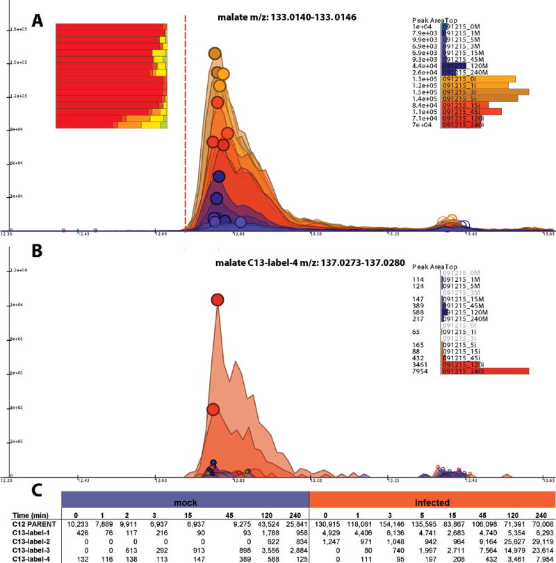
Visualization of raw LC–MS data. (A) Extracted ion chromatograms (EICs) for unlabeled malate (deprotonated anion). The red vertical line indicates the anticipated retention time of malate. The data comes from a ¹³C-glucose labeling time course in uninfected fibroblasts (blue) and HCMV infected ones (orange). The size of the filled circles on top of the peaks is proportional to the peak quality score. All of the peaks have large circles indicative of high peak quality. The bar chart on the right shows peak areas. The bar chart on the left shows the fraction of different labeled forms (red, unlabeled; orange-red, ¹³C₁; orange, ¹³C₂; yellow, ¹³C₃; yellow-green, ¹³C₄). The fractional labeling increases with longer labeling time. The increase is greater in the virally infected cells. Clicking on a bar corresponding to a labeled form brings up the associated set of EICs, as shown in part B for the fully labeled (¹³C₄) malate. Right clicking brings up the table of peak areas for all samples and labeling states, as shown in part C. This table can be exported to a spreadsheet via a mouse click.

The primary graphical interface of MAVEN is the EIC display shown in Figures 4 and 1B. For a given m/z slice, this interface shows the raw EIC for every sample. Figure 4A shows the m/z slice corresponding to unlabeled malate. The top point of every peak is marked by a circle. The size of the circles corresponds to the neural network-determined peak quality score, with large circles (as for malate) corresponding to high-quality peaks. For EICs containing the m/z of a known metabolite, a red vertical line marks the metabolite’s annotated retention time. Malate’s retention time is 12.7 min based on injection of purified standard.²¹

The upper right corner of the screen displays a bar graph of peak intensities. For each sample, there is a bar corresponding to the intensity of the peak closest to the annotated retention time. This bar graph allows the analyst to quickly see whether there is a trend in peak intensity across samples. Figure 4A shows that malate is ~10-fold more abundant in the virally infected cells. Clicking on a group of peaks at a different retention time automatically changes the bar graph to display the magnitudes of these peaks.

As each peak is examined, MAVEN also displays information relating to isotopic variants of the peak in the upper left corner of the screen. To enable this analysis, the user specifies any isotope labeling of the samples (¹³C, ¹⁵N, ³⁴S, etc.). This information allows MAVEN to compute the m/z values for all relevant isotopic forms. EICs are generated for each predicted isotopic variant. These EICs are limited to user specified retention time window (typically ±1 min) of the unlabeled peak. The peaks in isotopic EICs are grouped and scored as described above. Additionally, peak retention time match is calculated between the unlabeled peak and all isotopic peaks. The metric is the Pearson correlation of scan-by-scan signal intensities between the two peaks. Isotopic peaks are ignored if the peak shape match is inadequate (r < 0.1). This is a loose criterion that allows for minor retention time shifts due to isotope labeling but eliminates most erroneous peaks. Isotopic peaks are also rejected if their intensity is inconsistent with natural abundances given the user-entered isotope labeling. For example, assuming no isotope labeling (e.g., in the t) 0 sample in the ¹³C-glucose labeling time course), for a four-carbon compound like malate, the ¹³C₁ peak would be expected to have an intensity of 4% of the unlabeled peak. MAVEN would consider only peaks within ±50% of this value, e.g., within 2%-6% of the unlabeled peak intensity. In the event that multiple peaks meet the retention time, shape match, and intensity criteria, then the highest intensity of these is selected by MAVEN.

For each sample, a bar in graph in the upper left of the screen shows the fraction of the metabolite in different isotopic forms (unlabeled, ¹³C₁, ¹³C₂, etc.). Examination of these bar graphs in Figure 4A reveals progressive labeling of malate over time after the switch to ¹³C-glucose. The labeling is both more extensive and rapid in the virally infected cells, consistent with their having enhanced anapleurotic and TCA cycle flux. Clicking on an isotopic form pulls up the associated EIC, with the EICs for ¹³C₄ malate (i.e., fully labeled malate) shown in Figure 4B. If the incorrect isotope-labeled peak has been selected, e.g., due to a high intensity interfering peak in the isotopic EIC, then the user can click on the correct peak to fix the error. The labeling bar graph is automatically updated with the new information.

When the user is satisfied that all peak annotations are correct, then the resulting peak intensity data for the unlabeled and isotopic peaks can be exported to a spreadsheet (XML or CSV format) via a single mouse click. In the exported data matrix, samples are columns, compounds (EIC peaks) are rows, and matrix entries are peak intensities. Extracted data for malate is shown in Figure 4C.

Adducts and fragments are pulled out in the similar manner to isotopic peaks. MAVEN contains a list of typical adducts and fragments for positive and negative mode electrospray ionization.²¹ Because adducts arise directly in the ion source, peak overlap with the [M − H]⁻ or [M + H]⁺ peak should be high. Accordingly, a more stringent peak shape match threshold (typically r > 0.5) is used for adducts than for isotopes.

Pathway and Isotope-Labeling Visualization

To convert metabolomic data into useful knowledge, mapping the data onto known metabolic pathways is critical.^25–27 MAVEN contains a built-in pathway visualization interface. In the interface, compounds appear as circular nodes and reactions as arrows between nodes. Compounds, reactions, and pathway layouts can be loaded from established sources such as KEGG²⁸ and Metacyc.²⁹ The layout of pathways graphs can be adjusted by clicking and dragging. New reactions, compounds, and pathways can be entered and linked to existing pathways.

For all pathway compounds, MAVEN will calculate EICs, extract peaks, and display pool size or labeling information. The user can adjust the information displayed through a series of menu selections. One option is to display peak intensity data as the size of the metabolite nodes in the pathway graph. Another is to color-code the nodes based on whether the metabolite peak intensity increases or decreases in an experimental condition. Yet another option is to convert each node into a two-piece pie-chart, with the pie slices reflecting the fraction of isotope-labeled versus unlabeled metabolite. These options can be combined, so that, for example, a high-abundance metabolite that increases during viral infection appears as a large red node, whereas a low-abundance metabolite that does not change during viral infection appears as a small black node. Often visualization of data in the pathway context will reveal surprises, which may reflect peak misannotation or novel biology. To check peak assignments, users can pull up the raw data associated with any node simply by clicking on it.

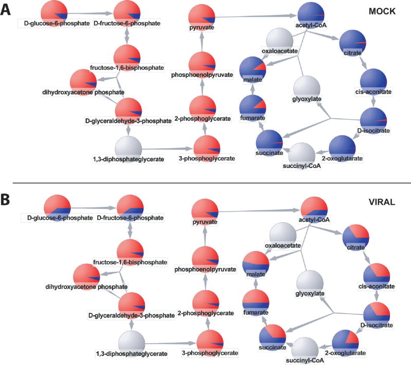
An example of visualization of isotope-labeling data is shown in Figure 5. The glycolysis/TCA cycle superpathway diagram was downloaded from Metacyc. Data are displayed for mock infected and virally infected samples after 1 h of ¹³C-glucose labeling. Each node in the diagram is a pie graph, with the red slice corresponding to the fraction of the total metabolite pool that that is ¹³C-labeled. Examining the glycolytic pathway reveals similarly extensive labeling in both the mock and virally infected cells. In contrast, for acetyl-CoA and the TCA cycle, labeling is much more extensive in the virally infected cells. This is consistent with cytomegalovirus up-regulating pyrvuate dehydrogenase and TCA cycle flux. One compound showing a strong up-regulation of labeling during viral infection is acetyl-CoA. In addition to being a driver of TCA flux, acetyl-CoA is the carbon source for fatty acid synthesis. Intriguingly, inhibitors of fatty acid biosynthesis inhibit human cytomegalovirus replication.²⁴ Thus visualization of labeling data within a pathway context provides a starting point for drawing medically relevant hypotheses from metabolomic data.

Figure 5.

Pathway-based visualization of isotope-labeling data. The pie graphs show the fraction of each compound that is isotope labeled (red) after 1 h of feeding U–¹³C-glucose. (A) Uninfected human fibroblasts. (B) Cytomegalovirus infection with U–¹³C-glucose introduced at 48 h post infection. The virus up-regulates flux through acetyl-CoA and the TCA cycle. While supporting the same qualitative biological conclusions, these data differ somewhat from those of Munger et al.²⁴ because here we used primary fibroblasts as the host cell, versus previously an immortalized fibroblast cell line. Animated movies showing the temporal progression of labeling are available as Supporting Information.

In many cases, drawing the correct inferences involves understanding the temporal evolution of metabolic changes (or labeling events). To this end, MAVEN will assemble not just single pathway graphs, as shown in Figure 5, but temporal series of such graphs. Users can click through the series of graphs to get a sense of time-evolution of the system. For example, Supplementary Movie 1 in the Supporting Information shows glycolysis and TCA cycle labeling at 0, 1, 3, 5, 10, 30, 45, 120, and 240 min following ¹³C-glucose addition. The labeling dynamics support the impression that flux through acetyl-CoA and the TCA cycle is markedly increased in the human cytomegalovirus-infected cells.

Pairwise Sample Comparison

For known metabolites, visualization within the context of pathways makes sense. To discover novel metabolites, however, alternative ways of LC–MS data visualization are useful.³⁰ One approach involves looking at all peaks, known or unknown, and how they differ between two sets of samples. Peaks that change greatly in response to a particular biological perturbation (e.g., addition of a drug or modulation of a gene) are candidates for further workup. To identify such peaks, MAVEN uses a straightforward statistical approach: after peak detection and grouping, differences in peak intensity between the two sets of samples are evaluated by an unequal variance t test. Rather than relying on a normal distribution to convert the resulting t-statistics into p-values, MAVEN uses a bootstrapping approach: data sets are permuted, features randomly selected, and the resulting t-statistics used to generate a distribution of t-statistics under the null hypothesis. P-values are then assigned from t-statistics based on this distribution and FDR corrected using the linear step-up procedure. ³¹

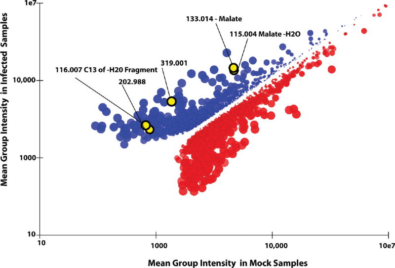
To visualize the data, a scatter plot is used. Each data point corresponds to a particular peak group, with the mean peak intensity in one sample set on the X-axis, and in the other sample set on the Y-axis. The sizes of the data points are proportional to fold difference between mean intensities of the two sets. The intensity of color of the data points reflects the statistical significance of the between-group difference: they are proportional to the boot-strapped, FDR-corrected p-value. The plot is interactive. Clicking once on any point on the plot highlights coeluting peak groups that are likely fragments, adducts, or isotope-labeled forms of the selected peak. Double clicking takes the analyst to the raw EICs of the highlighted peak group.

An example of pairwise sample comparison, for the uninfected versus virally infected fibroblast samples, is shown in Figure 6. The highlighted peak, shown in yellow, corresponds to malate, which increases ~10-fold during viral infection (p < 0.0025). There are other peaks that show yet larger changes; these peaks correspond to unexpected or structurally novel metabolites, whose identities we are currently working on confirming. With the malate peak clicked on, associated peaks that coelute and thus are likely to be adducts or fragments have been highlighted in yellow. The identities of some of these peaks have subsequently been manually annotated.

Figure 6.

Pairwise sample comparison. Each point corresponds to a peak group, with the X-value the mean peak intensity in uninfected samples and the Y-value the mean peak intensity in virally infected samples. The size of the points is proportional to fold difference between mean intensities. Points are colored red if the mean peak intensity in set 1 (mock) is greater than the mean in set 2 (viral). The intensity of color is proportional to p-values, based on the formula below. Only groups with at least a 2-fold difference are shown. Highlighted in yellow are groups corresponding to isotopes, potential adducts, and fragments of malate. Clicking on the point corresponding to malate leads to automatic highlighting of these related compounds. The color intensity equals to 1.0 – (p-value^0.2).

CONCLUSIONS

MAVEN builds on the capabilities of existing open-source software for LC–MS data analysis, such as XCMS, by providing interactive tools for data validation and visualization. Key attributes of MAVEN are carefully designed graphical interfaces; easy navigation between raw data and advanced graphics (e.g., pathway views); and underlying algorithms that make most software responses instantaneous from the user perspective. In addition to LC–MS data, MAVEN also can process multiple reaction monitoring (MRM) data; in this case, each MRM scan corresponds to an EIC. Efforts to incorporate full scan MS/MS data (e.g., from tandem quadrupole/time-of-flight instruments) are ongoing.

References

- 1.Fiehn O. Plant. Mol. Biol. 2002;48(1–2):155–171. [PubMed] [Google Scholar]
- 2.Vinayavekhin N, Homan EA, Saghatelian A. ACS. Chem. Biol. 2010;5(1):91–103. doi: 10.1021/cb900271r. [DOI] [PubMed] [Google Scholar]
- 3.Holmes E, Wilson ID, Nicholson JK. Cell. 2008;134(5):714–717. doi: 10.1016/j.cell.2008.08.026. [DOI] [PubMed] [Google Scholar]
- 4.Wishart DS. Drugs R&D. 2008;9(5):307–322. doi: 10.2165/00126839-200809050-00002. [DOI] [PubMed] [Google Scholar]
- 5.Metz TO, Zhang Q, Page JS, Shen Y, Callister SJ, Jacobs JM, Smith RD. Biomarkers Med. 2007;1(1):159–185. doi: 10.2217/17520363.1.1.159. [DOI] [PMC free article] [PubMed] [Google Scholar]
- 6.Dettmer K, Aronov PA, Hammock BD. Mass Spectrom. Rev. 2007;26(1):51–78. doi: 10.1002/mas.20108. [DOI] [PMC free article] [PubMed] [Google Scholar]
- 7.Sreekumar A, Poisson LM, Rajendiran TM, Khan AP, Cao Q, Yu J, Laxman B, Mehra R, Lonigro RJ, Li Y, Nyati MK, Ahsan A, Kalyana-Sundaram S, Han B, Cao X, Byun J, Omenn GS, Ghosh D, Pennathur S, Alexander DC, Berger A, Shuster JR, Wei JT, Varambally S, Beecher C, Chinnaiyan AM. Nature. 2009;457(7231):910–914. doi: 10.1038/nature07762. [DOI] [PMC free article] [PubMed] [Google Scholar] [Research Misconduct Found]
- 8.Smith CA, Want EJ, O’Maille G, Abagyan R, Siuzdak G. Anal. Chem. 2006;78(3):779–87. doi: 10.1021/ac051437y. [DOI] [PubMed] [Google Scholar]
- 9.Karpievitch YV, Hill EG, Smolka AJ, Morris JS, Coombes KR, Baggerly KA, Almeida JS. Bioinformatics. 2007;23(2):264–5. doi: 10.1093/bioinformatics/btl583. [DOI] [PMC free article] [PubMed] [Google Scholar]
- 10.Benton HP, Wong DM, Trauger SA, Siuzdak G. Anal. Chem. 2008;80(16):6382–6389. doi: 10.1021/ac800795f. [DOI] [PMC free article] [PubMed] [Google Scholar]
- 11.Katajamaa M, Oresic M. J. Chromatogr., A. 2007;1158(1–2):318–328. doi: 10.1016/j.chroma.2007.04.021. [DOI] [PubMed] [Google Scholar]
- 12.Reinert K, Kohlbacher O. Methods Mol. Biol. (Clifton, NJ) 2010;604:201–211. doi: 10.1007/978-1-60761-444-9_14. [DOI] [PubMed] [Google Scholar]
- 13.Pluskal T, Castillo S, Villar-Briones A, Oresic M. BMC Bioinf. 2010;11(1):395. doi: 10.1186/1471-2105-11-395. [DOI] [PMC free article] [PubMed] [Google Scholar]
- 14.Wikoff WR, Anfora AT, Liu J, Schultz PG, Lesley SA, Peters EC, Siuzdak G. Proc. Natl. Acad. Sci. U.S.A. 2009;106(10):3698–3703. doi: 10.1073/pnas.0812874106. [DOI] [PMC free article] [PubMed] [Google Scholar]
- 15.Romero R, Mazaki-Tovi S, Vaisbuch E, Kusanovic JP, Chaiworapongsa T, Gomez R, Nien JK, Yoon BH, Mazor M, Luo J, Banks D, Ryals J, Beecher C. J. Matern.-Fetal Neonat. Med. 2010 doi: 10.3109/14767058.2010.482618. [DOI] [PMC free article] [PubMed] [Google Scholar]
- 16.Dang L, White DW, Gross S, Bennett BD, Bittinger MA, Driggers EM, Fantin VR, Jang HG, Jin S, Keenan MC, Marks KM, Prins RM, Ward PS, Yen KE, Liau LM, Rabinowitz JD, Cantley LC, Thompson CB, Vander Heiden MG, Su SM. Nature. 2010;465(7300):966. doi: 10.1038/nature09132. [DOI] [PMC free article] [PubMed] [Google Scholar]
- 17.Boer VM, Crutchfield CA, Bradley PH, Botstein D, Rabinowitz JD. Mol. Biol. Cell. 2009;21(1):198–211. doi: 10.1091/mbc.E09-07-0597. [DOI] [PMC free article] [PubMed] [Google Scholar]
- 18.Kell DB. Curr. Opin. Microbiol. 2004;7(3):296–307. doi: 10.1016/j.mib.2004.04.012. [DOI] [PubMed] [Google Scholar]
- 19.Zamboni N, Fendt S-M, Ru¨hl M, Sauer U. Nat. Protoc. 2009;4(6):878–892. doi: 10.1038/nprot.2009.58. [DOI] [PubMed] [Google Scholar]
- 20.Yuan J, Bennett BD, Rabinowitz JD. Nat. Protoc. 2008;3(8):1328–1340. doi: 10.1038/nprot.2008.131. [DOI] [PMC free article] [PubMed] [Google Scholar]
- 21.Lu W, Clasquin MF, Melamud E, Amador-Noguez D, Caudy AA, Rabinowitz JD. Anal. Chem. 2010;82(8):3212–3221. doi: 10.1021/ac902837x. [DOI] [PMC free article] [PubMed] [Google Scholar]
- 22.Katajamaa M, Miettinen J, Oresic M. Bioinformatics. 2006;22(5):634–636. doi: 10.1093/bioinformatics/btk039. [DOI] [PubMed] [Google Scholar]
- 23.Tautenhahn R, Bo¨ttcher C, Neumann S. BMC Bioinf. 2008;9:504–504. doi: 10.1186/1471-2105-9-504. [DOI] [PMC free article] [PubMed] [Google Scholar]
- 24.Munger J, Bennett BD, Parikh A, Feng X-J, McArdle J, Rabitz HA, Shenk T, Rabinowitz JD. Nat. Biotechnol. 2008;26(10):1179–1186. doi: 10.1038/nbt.1500. [DOI] [PMC free article] [PubMed] [Google Scholar]
- 25.Xu EY, Schaefer WH, Xu Q. Curr. Opin. Drug Discovery Dev. 2009;12(1):40–52. [PubMed] [Google Scholar]
- 26.Droste P, Weitzel M, Wiechert W. Bioprocess. Biosyst. Eng. 2008;31(3):227–39. doi: 10.1007/s00449-007-0177-1. [DOI] [PubMed] [Google Scholar]
- 27.Gao J, Tarcea VG, Karnovsky A, Mirel BR, Weymouth TE, Beecher CW, Cavalcoli JD, Athey BD, Omenn GS, Burant CF, Jagadish HV. Bioinformatics. 2010;26(7):971–973. doi: 10.1093/bioinformatics/btq048. [DOI] [PMC free article] [PubMed] [Google Scholar]
- 28.Kanehisa M, Araki M, Goto S, Hattori M, Hirakawa M, Itoh M, Katayama T, Kawashima S, Okuda S, Tokimatsu T, Yamanishi Y. Nucleic Acids Res. 2008;36(suppl_1):D480–484–D480–484. doi: 10.1093/nar/gkm882. [DOI] [PMC free article] [PubMed] [Google Scholar]
- 29.Caspi R, Foerster H, Fulcher CA, Kaipa P, Krummenacker M, Latendresse M, Paley S, Rhee SY, Shearer AG, Tissier C, Walk TC, Zhang P, Karp PD. Nucleic Acids Res. 2008;36(suppl_1):D623–631–D623–631. doi: 10.1093/nar/gkm900. [DOI] [PMC free article] [PubMed] [Google Scholar]
- 30.Broadhurst D, Kell D. Metabolomics. 2006;2(4):171–196. [Google Scholar]
- 31.Benjamini Y, Hochberg Y. J. R. Stat. Soc., Ser. B (Methodol.) 1995;57(1):289–300. [Google Scholar]
Associated Data
This section collects any data citations, data availability statements, or supplementary materials included in this article.