Structured Learning for 3D Perivascular Spaces Segmentation Using Vascular Features

Abstract

Objective

The goal of this paper is to automatically segment perivascular spaces (PVSs) in brain from high-resolution 7T MR images.

Methods

We propose a structured-learning-based segmentation framework to extract the PVSs from high-resolution 7T MR images. Specifically, we integrate three types of vascular filter responses into a structured random forest for classifying voxels into two categories, i.e., PVS and background. In addition, we propose a novel entropy-based sampling strategy to extract informative samples in the background for training an explicit classification model. Since the vascular filters can extract various vascular features, even thin and low-contrast structures can be effectively extracted from noisy backgrounds. Moreover, continuous and smooth segmentation results can be obtained by utilizing patch-based structured labels.

Results

The performance of our proposed method is evaluated on 19 subjects with 7T MR images, with the Dice similarity coefficient reaching 66%.

Conclusion

The joint use of entropy-based sampling strategy, vascular features, and structured learning can improve the segmentation accuracy.

Significance

Instead of manual annotation, our method provides an automatic way for PVS segmentation. Moreover, our method can be potentially used for other vascular structure segmentation because of its data-driven property.

I. Introduction

Perivascular spaces (PVSs), which are also known as Virchow-Robin spaces, are cerebrospinal fluid (CSF) filled spaces ensheathing small blood vessels as they penetrate the brain parenchyma [1]. The clinical significance of PVSs comes primarily from their tendency to dilate in abnormal cases. For example, normal brains show a few dilated PVSs, while an increase of dilated PVSs has been shown to correlate with the incidence of several neurodegenerative diseases, making PVS a notably important area of research [2], [3], [4], [5]. Particularly, substantial research based on dilated PVS has been used for the diagnosis of Alzheimer’s disease [6], stroke [7], multiple sclerosis [8], and autism [9]. In general, most of the current studies require the precise segmentation of PVSs to calculate quantitative measurements. However, manual annotation of PVSs is tedious and time-consuming. Therefore, accurate and automatic segmentation of PVSs is highly desirable in PVS-based studies.

Since PVSs are vessel-like structures, many general vessel segmentation approaches can be potentially applied to PVS segmentation. These methods can be roughly divided into two categories, i.e., unsupervised method and supervised method. Most of the unsupervised methods are based on the edge enhancement or detection. For example, the first-order intensity variation detectors (e.g., Canny edge detector [10]), second order intensity variation detectors (e.g., Frangi filters [11]), curvilinear detectors (e.g., stick filter [12], and optimally oriented flux (OOF) [13]) are prevalently used for vessel enhancement and detection. Based on the enhanced vessel structure, target vessels can be segmented by thresholding [14], [15], clustering [16], or active contour modeling [17]. So far, only a few studies have focused on automatic PVS segmentation from MR images in an unsupervised manner. For example, Descombes et al. [18] enhanced the PVSs with filters and used a region-growing approach to get initial segmentation, followed by a geometry prior constraint for further improving the segmentation accuracy. Wuerfel et al. [4] segmented the PVSs with a semi-automatic software by adjusting intensity threshold. Uchiyama et al. [19] adopted a gray-level thresholding technique to extract PVSs from MR images, where these images were first enhanced by a morphological white top-hat transformation. However, the segmentation performance is usually limited with these unsupervised techniques, since it is very challenging to distinguish PVSs from confounding tissue boundaries.

On the other hand, supervised methods have demonstrated superiority in vessel segmentation by using powerful classifiers. For example, Ricci and Perfetti [20] employed support vector machine (SVM) for retinal vessel segmentation with a special designed line detector. Marín et al. [21] adopted neural network (NN) for retinal vessel segmentation with gray-level and moment invariants based features. Schneider et al. [22] used random forest (RF) for vessel segmentation from rat visual cortex images with rotation invariant steerable features.

However, there are several challenges for directly applying these supervised learning methods to PVS segmentation: 1) Since PVSs are extremely narrow and have low contrast compared with their neighboring tissues (see Fig. 1), general features may not be able to capture the discriminative characteristics of PVSs given confounding background. 2) Informative tubular structures of PVSs cannot be considered in conventional supervised learning methods, thus often leading to discontinuous and unsmooth segmentation results. However, using a simple global geometrical constraint may cause overfitting, since PVSs can appear at any location and also have large shape variations (e.g., different lengths, widths, and curvatures). 3) The number of PVS voxels is smaller than that of background voxels, while there are also enormous amounts of uninformative voxels in the background, which makes it difficult to train a reliable classifier with conventional random voxel sampling methods.

Fig. 1.

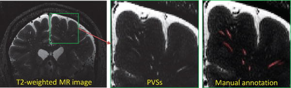
PVSs in the T2-weighted MR images.

To address these challenges, we propose a structured-learning-based framework for PVS segmentation using high-resolution 7T MR images. Specifically, we first introduce an entropy-based sampling strategy to remove redundant voxels in the background. From the informative samples, we extract three types of vascular features, based on steerable filters, Frangi filter, and OOF, to capture various characteristics of PVSs and their neighborhoods. We integrate these feature responses into a structured RF (SRF) to classify voxels into positive (i.e., PVS) and negative (i.e., background) classes. The structured RF effectively utilizes the patch based structured labels in the training stage, which allows for continuous and smooth segmentation in our method.

The remaining sections are organized as follows. Section II introduces the data used in this paper. Section III describes our PVS segmentation procedure, including region-of-interest generation, voxel sampling, feature extraction, and classification using SRF. Section IV reports experimental results and compares our method with other thresholding-based methods. In Section V, several important phenomena caused by replacing components of our method are discussed respectively. Finally, the conclusion is given in Section VI.

II. Materials

A 7T Siemens Scanner with a 32-channel head coil and a single-channel volume transmit coil (Nova Medical, Wilmington, MA) were used during our data acquisition.

Both T1- and T2-weighted 3D MR images were scanned for each subject with spatial resolution of 0.65 × 0.65 × 0.65mm³ and 0.5×0.5×0.5mm³ (or 0.4×0.4×0.4mm³), respectively. Specifically, the MPRAGE sequence [23] was adopted to acquire the T1-weighed images, with T E = 1.89ms and T R = 6000ms. The 3D variable flip angle turbo-spin echo sequence [24] was adopted to acquire the T2-weighted images, with T E = 457ms and T R = 5000ms for the resolution of 0.5× 0.5× 0.5mm³, or T E = 319ms and T R = 5000ms for the resolution of 0.4 × 0.4 × 0.4mm³.

In total, we acquired 19 image sets from 19 subjects. The manual segmentation was carried out by a MR scientist and a computer scientist specialized in image analysis. Both manual raters have more than 7 years research experience in image analysis. The segmentation procedure was repeated alternatively between these two manual raters until a final consensus is reached. The detailed procedure for generating manual segmentation was given in [25].

III. Method

In the previous work [25], we have focused on the MRI protocol optimization and the feasibility of characterizing PVS morphology from the optimized MR images. The segmentation of PVSs was obtained by manual correction of results obtained from a simple threshold-based method. In this paper, we focus on automatic segmentation of PVSs using structured learning and vascular features. As shown in Fig. 2, our method is comprised of two stages. In the training stage, we first generate a region-of-interest (ROI) using T1-weighted image. Then, we sample training voxels according to the probabilities calculated with local entropies using T2-weighted images. Next, the vascular features from T2-weighted images are extracted to describe the local structure of each voxel, and the patch-based structured labels are also extracted from the binary segmentation (PVS) maps as multiple target labels. We finally train a SRF model using those both vascular features and structured labels. In the testing stage, we first extract vascular features for each voxel in the ROI, and then feed these features into the pre-trained SRF model. In this way, the PVS segmentation can be performed in each testing image in a classification manner.

Fig. 2.

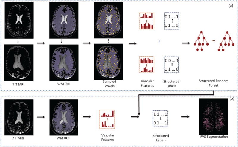
Schematic diagram of the proposed method. (a) Training stage. The WM ROI is first extracted. Then, the voxels are sampled with the proposed sampling strategy, followed by the vascular feature extraction and structured label extraction. Finally, SRF classifier is trained. (b) Testing stage. The WM ROI is first extracted. Then, the vascular features are extracted for all voxels within the ROI. The structured labels can be predicted using the trained classifier. Finally, the PVS voxels can be further determined using these predicted structured labels.

A. Region-of-interest Generation

In this paper, we focus only on the PVSs within white matter (WM), which plays an important role in the clearance of metabolic wastes from the brain. Moreover, T2-weighted MRI is the best modality to identify all PVSs [26]. Therefore, we extract the WM tissue in the T2-weighted image as our ROI for PVS segmentation. Since image contrast between WM and gray matter (GM) is clearer in the T1-weighted image rather than the T2-weighted image, we first rigidly align the T1-weighted image to the T2-weighted image, and then perform skull stripping and WM tissue segmentation on the aligned T1-weighted image. Accordingly, we can obtain the WM segmentation in the T2-weighted image space. Specifically, we adopt FLIRT [27], [28], BET [29] and FAST [30] tools from FSL [31] to implement the aforementioned rigid alignment, skull stripping, and tissue segmentation, respectively.

B. Voxel Sampling Strategy

In general, the number of PVS voxels is much smaller (i.e., ranging from several thousands to tens of thousands) than the total number of voxels in the WM (i.e., millions). To avoid class-imbalanced problem, we select all PVS voxels as positive samples, and use only a small portion of voxels in the background as negative samples. Since the background includes a large number of uninformative (or less informative) voxels from the uniform regions while a relatively small number of informative voxels, it is not reasonable to randomly sample the negative samples from background. In order to balance the proportions of uninformative (or less informative) and informative voxels, we propose to sample the voxels according to the probabilities calculated by local entropies around voxels in the background, as shown in Fig. 3.

Fig. 3.

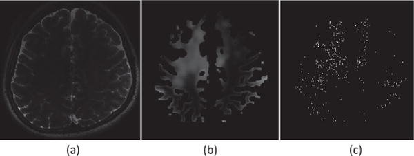
Sampling procedure. (a) T2-weighted image. (b) Entropy map within the ROI of white matter. (c) Sampled voxels from background.

Specifically, for a region around a specific voxel $\widehat{\eta }$, the local entropy $E\left(\widehat{\eta }\right)$ is defined as

$$E(\widehat{\eta })=-{\displaystyle \sum _i{p}_i(s,\widehat{\eta })\text{log}{p}_i(s,\widehat{\eta })},$$ (1)

where i is a possible intensity value, and $p_i(s,\widehat{\eta })$ is the probability distribution of intensity i within a spherical region $\mathrm{\Omega }(s,\widehat{\eta })$ centered at $\widehat{\eta }$ with a radius of s. That is, a larger value of $E(\widehat{\eta })$ denotes that the voxel $\widehat{\eta }$ is more informative.

Then, we sample the voxel $\widehat{\eta }$ with the probability of $P(\widehat{\eta })$, which is defined as

$$P(\widehat{\eta })=e^{-\frac{\omega }{E(\widehat{\eta })}},$$ (2)

where ω is a coefficient used to directly adjust the sampling probability and also control the total number of sampled voxels. In doing so, most of the informative voxels can be sampled from background.

C. Feature Extraction

For many vessel segmentation problems, the orientations of the vessels (e.g., retinal vessels and pulmonary vessels) are generally irregular. Therefore, the orientation invariance is an important property of features. However, unlike conventional vessel segmentation problems, PVSs have roughly regular orientations that point to ventricles filled with CSF, as shown in Fig. 2 (b) (PVS segmentation). Considering the useful orientation information of PVSs, we extract three types of vascular features based on three filters (steerable filters, Frangi filter, and OOF) from T2-weighted images. For each type of these features, we also employ multi-scale representation to capture both coarse and fine structural features.

1) Steerable-Filter-based Features

Since Gaussian derivative filters are steerable, any arbitrary oriented responses of the first-order and second-order Gaussian derivative filters can be obtained by the linear combinations of some basis filter responses [32], [33]. Due to the selective band-pass property of the first-order and second-order Gaussian derivative filters, the steerable filters are prevalent for extracting local features [34], [35], [36]

Assume the definition of a basic Gaussian-like filter G as:

$$G(x,y,z)=e^{\frac{-(x^2+y^2+z^2)}{{\sigma }^2}},$$ (3)

where σ² is the variance of this Gaussian-like filter. The basis filters for the first derivative and second derivative Gaussian filters are the first and second derivatives with respect to the three coordinate directions (x, y, z), respectively, i.e., G_x, G_y, G_z, G_xx, G_xy, G_xz, G_yy, G_yz, and G_zz.

On the other hand, give an arbitrary orientation $\widehat{\theta }=(\alpha ,\beta ,\mathrm{\gamma })$, which is defined by spherical coordinates (θ, ϕ) as follows:

$$\alpha =\mathit{cos}(\theta )\mathit{sin}(\varphi ),\beta =\mathit{sin}(\theta )\mathit{sin}(\varphi ),\mathrm{\gamma }=\mathit{cos}(\varphi ).$$ (4)

Considering the symmetry of filters, we let θ ∈ [0, π] and π ∈ [0, π]. Therefore, the oriented first-order derivative of Gaussian filter can be calculated as:

$$G_{\widehat{\theta }}=\alpha G_x+\beta G_y+\mathrm{\gamma }{G}_z.$$ (5)

The oriented second-order derivative of Gaussian filter can be calculated as:

$$G_{2\widehat{\theta }}={\alpha }^2{G}_{xx}+{\beta }^2{G}_{yy}+{\mathrm{\gamma }}^2{G}_{zz}+2\alpha \beta G_{xy}+2\alpha \mathrm{\gamma }{G}_{xz}+2\beta \mathrm{\gamma }{G}_{yz}.$$ (6)

Since all basis filters are x – y − z separable, the three dimensional convolution can be implemented by three one-dimensional convolutions on the directions of x, y, and z successively. In doing so, it is efficient to get their filtering responses. In this study, we extract the 3D steerable-filter-based features including the responses of a Gaussian filter, 9 oriented first-order Gaussian derivative filters, and 9 orientated second-order Gaussian derivative filters. Therefore, there are 19 features for each scale of steerable filters (where the scale is defined by the standard deviation of Gaussian/Gaussian derivative filters).

2) Frangi-based Features

The Frangi-based measurements are extracted based on the Hessian matrix consisting of second-order derivative of Gaussian filter responses [11], and the Hessian matrix (H) can be written as:

$$H=\left[\begin{array}{ccc}I\ast G_{xx}& I\ast G_{xy}& I\ast G_{xz}\\ I\ast G_{yx}& I\ast G_{yy}& I\ast G_{yz}\\ I\ast G_{zx}& I\ast G_{zy}& I\ast G_{zz}\end{array}\right],$$ (7)

where ∗ is a convolution operator. Therefore, the three eigenvalues, i.e., γ₁ > γ₂ > γ₃, can be calculated based on the Hessian matrix. In our study, we first extract 3 features based on the eigenvalues, which are $\left(\frac{|{\mathrm{\gamma }}_1|}{|{\mathrm{\gamma }}_2|},\frac{|{\mathrm{\gamma }}_1|}{\sqrt{|{\mathrm{\gamma }}_2{\mathrm{\gamma }}_3|}},\sqrt{{\mathrm{\gamma }}_1^2+{\mathrm{\gamma }}_2^2+{\mathrm{\gamma }}_3^2}\right)$^. We also extract 2 orientation features based on the eigenvector (x₁, y₁, z₁) corresponding to the maximum eigenvalue γ₁, which are ( $\text{arcoss}(\frac{|z_1|}{\sqrt{x_1^2+y_1^2+z_1^2}})$, $\text{arctan}(\frac{y_1}{x_1})$). Therefore, there are 5 features for each scale of Gaussian derivative filters (here, the scale is defined by the standard deviation of Gaussian derivative filters).

3) Optimally Oriented Flux (OOF)-based Features

The OOF has been proven to be effective to enhance the curvilinear structures by quantifying the amount of projected image gradient flowing in or out of a local spherical region [13]. The OOF matrix (i.e., ${\mathbf{Q}}_{r,\widehat{\tau }}$) is a 3 × 3 matrix, with the entry (i.e., $q_{r,\widehat{\tau }}^{i,j}$ at i-th row and j-th column defined as:

$$q_{r,\widehat{\tau }}^{i,j}={\displaystyle {\int }_{\partial S_r}{v}_i(\widehat{\tau }+r\widehat{n})}{n}_{j}dA,$$ (8)

where $\widehat{\tau }$ is the voxel coordinate, S_r is a local spherical region with radius r, $\widehat{v}(\widehat{\tau })={(v_1(\widehat{\tau }),v_2(\widehat{\tau }),v_3(\widehat{\tau }))}^T$, is a gradient vector, $\widehat{n}={(n_1,n_2,n_3)}^T$ is the outward unit normal of ∂S_r, and dA is the infinitesimal area on ∂S_r.

The major difference between the Frangi-based features and OOF-based features is the computations of Hessian matrix and OOF matrix. Particularly, the eigenvalues and eigenvectors of OOF matrix are grounded on the analysis of image gradient on the local spherical surface.

We extract 4 features based on the first two eigenvalues (i.e., λ₁ and λ₂) of the OOF Hessian matrix, which are (λ₁, λ₂, $\sqrt{\mathit{max}(0,{\mathrm{\lambda }}_1{\mathrm{\lambda }}_2)}$, λ₁ + λ₂). Moreover, we extract 2 orientation features based on the eigenvector $(x_1^{{}^{\prime }},y_1^{{}^{\prime }},z_1^{{}^{\prime }})$ corresponding to the maximum eigenvalue λ₁, which are $(\text{arccos}(\frac{|z_1^{{}^{\prime }}|}{\sqrt{x_1^{{}^{\prime }2}+y_1^{{}^{\prime }2}+z_1^{{}^{\prime }2}}}),\text{arctan}(\frac{y_1^{{}^{\prime }}}{x_1^{{}^{\prime }}}))$. Therefore, there are 6 features for each scale of spherical region (where the scale is defined by the radius of spherical region in calculating the flux).

D. Classification Using Structured Random Forest

Random forest (RF) classifier is a combination of tree predictors [37]. For a general RF-based segmentation task, the input space corresponds to the extracted local appearance features around each voxel, and the output space corresponds to the label of that voxel. As a matter of fact, the PVSs have line-like structures such that the neighborhood labels have certain structured coherence. Therefore, we perform the structured learning strategy in our task, thus addressing the problem of learning a mapping where the input or output space may represent the complex morphological structures.

In our task, the output space can be structured, so that we utilize the structured patch-based labels (i.e., the cubic patch with a size of k × k × k) in the in output space. Specifically, in the training stage, we first extract vascular features for each voxel sampled from T2-weighted image, as well as a corresponding cubic label patch from manually segmented binary image. Then, a SRF (multi-label) model is trained using the features and labels. In the testing stage, we similarly extract the respective features for all voxels in the WM tissue from a testing T2-weighted image. Then, the features are fed to the trained SRF model, and each voxel outputs a labeled patch. By assigning the patch-based labels to the neighboring voxels, each voxel receives k³ label values, and we take the majority value as the final label for this voxel. Eventually, by using the structured labels, the local structural constraint of PVSs in the label space can be naturally incorporated into the SRF model.

In general, since most of PVSs point to the ventricles, PVSs within each hemisphere have roughly statistical regularity of orientations. To reduce the orientation divergence of PVSs, we learn two SRF models separately, with one for the left hemisphere and another for the right hemisphere. Finally, voxels from each hemisphere of the testing image are fed to the corresponding trained SRF model for labeling.

IV. Experiments

A. Parameter Setting

Two-fold cross validation is used to evaluate the segmentation performance. In order to expand the training dataset, each training image is further left-right flipped to generate one more training image. The parameters are set as follows. For white matter segmentation, we adopt default parameters for FLIRT, BET and FAST. For extracting multi-scale steerable-filter-based features, the standard deviations of Gaussian filters are set as [0.5, 1.5, 2.5, 3.5], thus obtaining 76 features in total. For extracting multi-scale OOF-based features, the flux radii are set as [0.5, 1, 1.5, 2, 2.5, 3, 3.5, 4], thus generating 48 features in total. For extracting Frangi-based features, the standard deviations of Gaussian filters are set as [0.5, 1, 1.5, 2, 2.5, 3, 3.5], thus obtaining 35 features in total. Here, we select slightly denser scales for generating OOF and Frangi-based features than steerable-filter-based features, to avoid the imbalance of different types of features. To extract patch-based labels, the patch size is set as 3×3×3. For voxel sampling, the radius s is set as 10, and the coefficient parameter ω is set as 15 to keep the proportion between positive voxels and negative voxels to be roughly 1:5. For training the SRF classifier, 10 independent trees are trained and the depth of each tree is set as 20.

B. Evaluation Criteria

In order to evaluate the segmentation performance, we define the following four performance measurements by comparing the predicted segmentation image with the manually annotated ground-truth. 1) True Positives (TP): predicted PVS voxels inside the ground-truth PVS segmentation. 2) False Positives (FP): predicted PVS voxels outside the ground-truth PVS segmentation. 3) True Negatives (TN): predicted background voxels outside the ground-truth PVS segmentation. 4) False Negatives (FN): predicted background voxels inside the ground-truth PVS segmentation.

Note that TN is generally a very large value compared with other measurements due to the severe unbalanced number of voxels (i.e., PVS vs. background). To avoid such influence, only the Dice similarity coefficient (DSC), sensitivity (SEN), and positive prediction value (PPV) are calculated as evaluation criteria, as shown below:

$$\mathit{DSC}=\frac{2TP}{2TP+FP+FN},\mathit{SEN}=\frac{TP}{TP+FN},\mathit{PPV}=\frac{TP}{TP+FP}.$$ (9)

In summary, DSC reflects the overall segmentation performance, SEN indicates the capability of detecting the PVS voxels, and PPV represents the capability of discarding the confounding background voxels.

C. Experimental Results

In our experiment, we compare our method with the methods of Frangi [11] and OOF [13] with a thresholding strategy, denoting as FT and OT, respectively. For the implementation of these two methods, we acquired the source codes from the websites in [38] and [39], respectively. For a fair comparison, we also pre-selected the ROI of WM for the two competing methods.

Table I and Fig. 4 show the segmentation results achieved by different methods. As can be seen, our method achieves the best result, compared with those two thresholding-based methods (i.e., FT and OT), demonstrating the effectiveness of our learning-based framework. We also shows the results using RF (not structured) and the vascular features. It can be seen that the use of SRF achieves roughly 6% improvement (in terms of DSC) as compared with the standard RF, and more than 14% (in terms of DSC) as compared with two thresholding-based methods.

TABLE I.

Segmentation results achieved by different methods. FT and OT indicate the thresholding-based method in [11] and [13], respectively. RF and SRF indicate the learning-based methods using random forest and structured random forest, respectively.

Subject	DC				SEN				PPV
	FT	OT	RF	SRF	FT	OT	RF	SRF	FT	OT	RF	SRF
1	0.534	0.535	0.591	0.661	0.511	0.512	0.519	0.615	0.559	0.560	0.686	0.716
2	0.539	0.572	0.619	0.679	0.537	0.570	0.580	0.657	0.542	0.574	0.664	0.703
3	0.553	0.573	0.607	0.643	0.566	0.586	0.598	0.636	0.541	0.560	0.615	0.650
4	0.518	0.555	0.635	0.659	0.565	0.602	0.623	0.651	0.478	0.515	0.648	0.668
5	0.544	0.547	0.582	0.635	0.570	0.572	0.599	0.633	0.520	0.523	0.566	0.636
6	0.526	0.527	0.614	0.623	0.571	0.569	0.589	0.590	0.487	0.490	0.663	0.708
7	0.464	0.464	0.590	0.691	0.494	0.535	0.555	0.695	0.410	0.421	0.630	0.687
8	0.480	0.481	0.533	0.644	0.481	0.479	0.492	0.662	0.480	0.482	0.597	0.626
9	0.467	0.493	0.551	0.631	0.488	0.535	0.565	0.625	0.449	0.458	0.539	0.637
10	0.444	0.481	0.585	0.646	0.515	0.589	0.630	0.699	0.390	0.406	0.546	0.597
11	0.518	0.519	0.572	0.638	0.490	0.495	0.526	0.616	0.549	0.552	0.676	0.688
12	0.469	0.503	0.641	0.685	0.512	0.545	0.589	0.695	0.433	0.467	0.704	0.675
13	0.542	0.546	0.618	0.700	0.568	0.579	0.590	0.709	0.523	0.525	0.647	0.682
14	0.433	0.445	0.588	0.624	0.517	0.518	0.570	0.614	0.373	0.425	0.608	0.663
15	0.451	0.454	0.582	0.653	0.490	0.482	0.547	0.631	0.418	0.422	0.620	0.676
16	0.536	0.539	0.622	0.636	0.558	0.547	0.583	0.596	0.515	0.522	0.667	0.682
17	0.513	0.517	0.643	0.695	0.567	0.545	0.573	0.641	0.491	0.484	0.733	0.758
18	0.573	0.583	0.658	0.715	0.573	0.582	0.645	0.704	0.573	0.583	0.673	0.726
19	0.556	0.555	0.627	0.705	0.590	0.593	0.635	0.702	0.525	0.520	0.620	0.710
Mean	0.508	0.520	0.603	0.661	0.535	0.549	0.579	0.651	0.487	0.499	0.637	0.679
Std	0.043	0.042	0.032	0.030	0.037	0.038	0.040	0.039	0.060	0.055	0.052	0.038

Fig. 4.

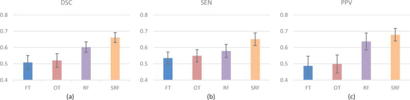
Quantitative evaluation of segmentation results compared with different methods. (a) DSC. (b) SEN. (c) PPV. FT and OT indicate the thresholding-based method in [11] and [13], respectively. RF and SRF indicate the learning-based methods using random forest and structured random forest, respectively.

Figure 4 (b) and (c) also show the corresponding SEN and PPV of different methods. By comparing these two criteria, we can observe two phenomena: 1) The PPVs achieved by the two thresholding-based segmentation methods (i.e., FT and OT) are much lower than those of the two learning-based methods (i.e., RF and SRF). 2) Compared with RF, SRF improves the segmentation performance more significant in SEN than PPV. That is, the PPV of RF is about 4 percent lower than that of SRF, while the SEN of RF is about 7 percent lower than that of SRF.

In order to give more evident explanation, we visualize the segmentation results of several typical PVSs in Fig. 5. 1) It is clear that the methods of FT and OT can detect most of the PVSs. The major problem of the two thresholding-based method is that they cannot distinguish the PVSs from the confounding tissue boundaries. Many confounding boundaries are wrongly classified as PVSs, leading to a large number of false positive voxels. However, the learning-based methods well solve such problem. Therefore, the PPVs of the two learning-based methods (i.e., RF and SRF) are significantly improved compared with those of the two thresholding-based methods. 2) The results achieved by RF model are generally better than those of two thresholding-based methods. However, the results of the RF model are often discontinuous and unsmooth. On the other hand, the SRF improves such circumstance because of the use of local structural constraint in the label space. Since there exist some PVS voxels that may be wrongly classified as background using RF (unstructured), the number of false negative voxels increases. This leads to a relatively low SEN of RF, compared with SRF.

Fig. 5.

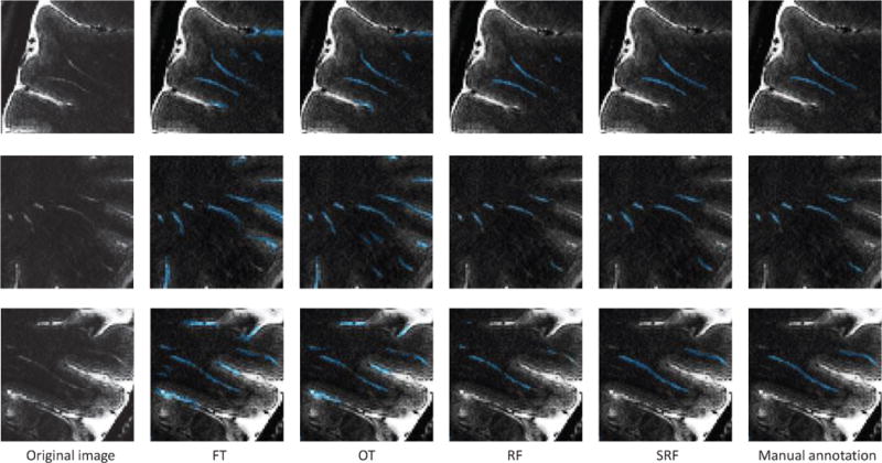
Illustrations of typical PVS segmentations.

V. Parameter Analysis and Discussions

A. Sampling Strategy

In our method, we sample voxels from background with their probabilities in proportion to the corresponding local entropies. For comparison, we show the result achieved by the method that simply randomly sample the voxels from background. As shown in Fig. 6, the proposed entropy-based sampling (ES) strategy improves the segmentation performance by more than 8% in terms of DSC for both RF and SRF classifiers. Figure 7 also shows several examples of PVS segmentations, by different sampling strategies. As indicated, random sampling strategy has potential risk of wrongly classifying the confounding boundary voxels as PVSs. Specifically, if we randomly sample the background voxels, many voxels that are similar to PVSs may not be sampled for training, due to the existence of much more uninformative voxels in background. On the other hand, the simple use of redundant unrepresentative sampled voxels for training may adversely affects the accuracy of classification model. As shown in Fig. 7, our method (i.e., ES+SRF) can distinguish voxels that are similar to the PVSs, but not PVSs, compared with random sampling strategy.

Fig. 6.

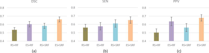
Comparison between different voxel sampling strategies. RS denotes the conventional random sampling strategy and ES denotes the proposed entropy-based sampling strategy. (a) DSC. (b) SEN. (c) PPV.

Fig. 7.

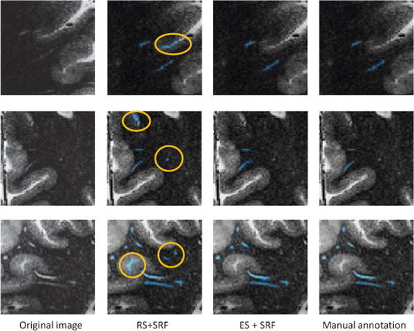
Illustration of segmentation results of using two different voxel sampling strategies. RS denotes the conventional random sampling strategy and ES denotes the proposed entropy-based sampling strategy. The falsely segmented PVSs are marked by circles.

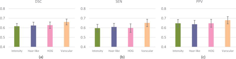
B. Vascular Features

We also conduct experiments by replacing the vascular features with patch-based intensity features, Haar-like features, and 3D HOG features [40]. For intensity feature extraction, the patch size is 11 × 11 × 11. For Haar-like features, we calculate differences between the sums of voxels of areas inside the cubic, which can be within a fixed patch with the size of 11×11×11. For HOG feature extraction, there are 16 orientations, and 2×2×2 cells, and each cell size is 5×5×5. For fair comparison, different types of features are separately used to train the corresponding SRF classifiers. Figure 8 shows that the best result is achieved using our vascular features. This can be attributed to the fact that vascular features can enhance vascular structures by removing potential noises.

Fig. 8.

Comparison among different features. (a) DSC. (b) SEN. (c) PPV.

C. Feature Scale Selection

One important parameter for feature extraction is the scale range for multi-scale representation. In our experiment, we define the scales of vascular features by their frequencies of being selected in all split nodes of a trained classification model. Specifically, we feed redundant features with many scales to train a classification model. Then, we count the frequencies of selected features in terms of their scales. As shown in Fig. 9, the distribution demonstrates the importance of each scale in extracting vascular features. Finally, we only use the scales in the reasonable range for each feature type, as introduced in our parameter setting part.

Fig. 9.

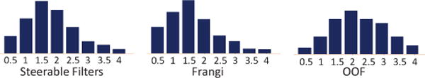
Frequencies of features being selected in different scales. The horizontal axis indicates the scale of each feature type. The vertical axis indicates the frequency of features being selected.

D. Effect of Noise

In this section, we analyze the robustness of our method with respect to noise. We add white Gaussian noise with zero mean and a certain standard deviation that depends on specific T2-weighted MR image, to obtain the expected signal to noise ratio (SNR). As shown in Fig. 10, both of the two learning-based methods (i.e., RF and SRF) are more robust to noise compared with the two thresholding-based methods (i.e., FT and OT). Moreover, it also suggests that our vascular features are more robust to the noise.

Fig. 10.

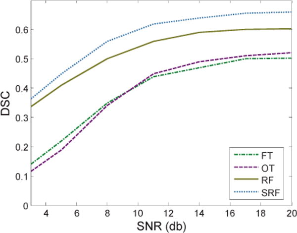
Segmentation results with respect to different noise levels.

E. Limitations of the Proposed Method

Although our method has improved the segmentation performance compared with existing thresholding-based methods, there are still some limitations. Figure 11 illustrates several cases of failed segmentations. As can be seen, there are some major types of failed situations. 1) One type of failed segmentation occurs on the PVSs close to the gray matter boundary (see the first row in Fig. 11). That may attribute to the fact that the patch appearance close to that PVS is not clear, and the strong filtering responses of boundary lead to ambiguous vascular features. Some high-level learning-based features (e.g., deep-learning-based features) may overcome such difficulty and then improve the segmentation performance. 2) It is difficult for our method to detect the PVSs with subject-specific shape structure (see the second row in Fig. 11). For the PVSs with their specific shape structures not included in the training dataset, they are not easily to detect, since our learning-based method is not heuristic. Such failures may be caused by the limited number of training subjects in our current study. Although we have flipped the training images in order to generate more training samples, the total number of training images is still limited. A potential way of solving this problem is to extend the training dataset by including the synthetic images with artificial variable-shape PVSs. 3) It is also difficult to detect too weak PVSs, although we have extracted vascular features to enhance vascular structures (see the third row in Fig. 11). Some enhancing and denoising techniques might be useful to preprocess images before our feature extraction stage.

Fig. 11.

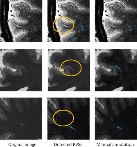
Illustration of failed segmentations. The failed segmentations are marked by circles.

Moreover, the imaging of PVSs is still an ongoing direction. Existing MR sequences may not show all PVSs, or the shown PVSs are still not easily to be manually annotated. Therefore, it is still very challenging to provide accurate ground-truth PVSs for training our model. The development of new MR sequence can potentially improve the imaging quality of PVSs, and thus provides more accurate ground truth, which can eventually improve our segmentation performance.

F. Future Work

In this paper, we focus only on the PVSs within the white matter, which plays an important role in the clearance of metabolic wastes from the brain. It may provide important insight into the pathophysiology of disease to understand the age dependent changes of PVS morphology within the white matter and also characterize its possible abnormality in Alzheimer’s disease and mild cognitive impairment. In our future work, instead of using the white-matter ROI, we will also segment the PVSs in whole brain, which may have broader clinical applications in intracerebral haemorrhage [41], Alzheimer’s disease [42], stroke [43], general elderly population analysis [44], and sleep [45].

In addition, we focus only on the PVS segmentation from MR images of young healthy volunteers, where few lacunar infarcts were present. Our method needs to be further improved for discriminating PVSs from small lacunar infarcts in the studies of PVSs in elderly subjects suffering from neurodegenerative diseases where lacunar infarcts are commonly observed [46]. One potential approach is to utilize different geometric shapes of the two structures, since PVSs have a linear structure while lacunar infarct is more isotropic. This will be our future research topic.

VI. Conclusion

In this paper, we have presented a structured-learning-based segmentation framework for PVS segmentation. Specifically, we defined vascular features to better distinguish PVSs from the complex background, and further used the patch-based structured labels to preserve local structure of segmented PVSs. Moreover, a novel voxel sampling strategy was proposed to further improve the segmentation performance. The experimental results indicated the superior segmentation performance of our proposed method in effective segmentation of PVSs.

References

- 1.Zhang E, et al. Interrelationships of the pia mater and the perivascular (Virchow-Robin) spaces in the human cerebrum. Journal of Anatomy. 1990;170:111. [PMC free article] [PubMed] [Google Scholar]
- 2.Esiri M, Gay D. Immunological and neuropathological significance of the virchow-robin space. Journal of the Neurological Sciences. 1990;100(1):3–8. doi: 10.1016/0022-510x(90)90004-7. [DOI] [PubMed] [Google Scholar]
- 3.MacLullich A, et al. Enlarged perivascular spaces are associated with cognitive function in healthy elderly men. Journal of Neurology, Neurosurgery & Psychiatry. 2004;75(11):1519–1523. doi: 10.1136/jnnp.2003.030858. [DOI] [PMC free article] [PubMed] [Google Scholar]
- 4.Wuerfel J, et al. Perivascular spaces–MRI marker of inflammatory activity in the brain? Brain. 2008;131(9):2332–2340. doi: 10.1093/brain/awn171. [DOI] [PubMed] [Google Scholar]
- 5.Rouhl R, et al. Virchow-robin spaces relate to cerebral small vessel disease severity. Journal of Neurology. 2008;255(5):692–696. doi: 10.1007/s00415-008-0777-y. [DOI] [PubMed] [Google Scholar]
- 6.Chen W, et al. Assessment of the virchow-robin spaces in Alzheimer disease, mild cognitive impairment, and normal aging, using high-field MR imaging. American Journal of Neuroradiology. 2011;32(8):1490–1495. doi: 10.3174/ajnr.A2541. [DOI] [PMC free article] [PubMed] [Google Scholar]
- 7.Selvarajah J, et al. Potential surrogate markers of cerebral microvascular angiopathy in asymptomatic subjects at risk of stroke. European Radiology. 2009;19(4):1011–1018. doi: 10.1007/s00330-008-1202-8. [DOI] [PubMed] [Google Scholar]
- 8.Etemadifar M, et al. Features of virchow-robin spaces in newly diagnosed multiple sclerosis patients. European Journal of Radiology. 2011;80(2):e104–e108. doi: 10.1016/j.ejrad.2010.05.018. [DOI] [PubMed] [Google Scholar]
- 9.Boddaert N, et al. MRI findings in 77 children with non-syndromic autistic disorder. PLoS One. 2009;4(2):e4415. doi: 10.1371/journal.pone.0004415. [DOI] [PMC free article] [PubMed] [Google Scholar]
- 10.Canny J. A computational approach to edge detection. IEEE Transactions on Pattern Analysis and Machine Intelligence. 1986;(6):679–698. [PubMed] [Google Scholar]
- 11.Frangi AF, et al. Multiscale vessel enhancement filtering. Medical Image Computing and Computer-Assisted Interventation Springer. 1998:130–137. [Google Scholar]
- 12.Xiao C, et al. Pulmonary fissure detection in CT images using a derivative of stick filter. 2016 doi: 10.1109/TMI.2016.2517680. [DOI] [PubMed] [Google Scholar]
- 13.Law MW, Chung AC. Computer Vision–ECCV 2008. Springer; 2008. Three dimensional curvilinear structure detection using optimally oriented flux,” in; pp. 368–382. [Google Scholar]
- 14.Hoover A, et al. Locating blood vessels in retinal images by piecewise threshold probing of a matched filter response. IEEE Transactions on Medical Imaging. 2000;19(3):203–210. doi: 10.1109/42.845178. [DOI] [PubMed] [Google Scholar]
- 15.Roychowdhury S, et al. Iterative vessel segmentation of fundus images. IEEE Transactions on Biomedical Engineering. 2015;62(7):1738–1749. doi: 10.1109/TBME.2015.2403295. [DOI] [PubMed] [Google Scholar]
- 16.Mohammadi Saffarzadeh V, et al. Vessel segmentation in retinal images using multi-scale line operator and k-means clustering. Journal of Medical Signals and Sensors. 2014;4(2):122–129. [PMC free article] [PubMed] [Google Scholar]
- 17.Florin C, et al. European Conference on Computer Vision. Springer; 2006. Globally optimal active contours, sequential monte carlo and on-line learning for vessel segmentation; pp. 476–489. [Google Scholar]
- 18.Descombes X, et al. An object-based approach for detecting small brain lesions: application to virchow-robin spaces. IEEE Transactions on Medical Imaging. 2004;23(2):246–255. doi: 10.1109/TMI.2003.823061. [DOI] [PubMed] [Google Scholar]
- 19.Uchiyama Y, et al. Engineering in Medicine and Biology Society. IEEE; 2008. Computer-aided diagnosis scheme for classification of lacunar infarcts and enlarged virchow-robin spaces in brain MR images,” in; pp. 3908–3911. [DOI] [PubMed] [Google Scholar]
- 20.Ricci E, Perfetti R. Retinal blood vessel segmentation using line operators and support vector classification. IEEE Transactions on Medical Imaging. 2007;26(10):1357–1365. doi: 10.1109/TMI.2007.898551. [DOI] [PubMed] [Google Scholar]
- 21.Marín D, et al. A new supervised method for blood vessel segmentation in retinal images by using gray-level and moment invariants-based features. IEEE Transactions on Medical Imaging. 2011;30(1):146–158. doi: 10.1109/TMI.2010.2064333. [DOI] [PubMed] [Google Scholar]
- 22.Schneider M, et al. Joint 3-D vessel segmentation and centerline extraction using oblique hough forests with steerable filters. Medical Image Analysis. 2015;19(1):220–249. doi: 10.1016/j.media.2014.09.007. [DOI] [PubMed] [Google Scholar]
- 23.Mugler JP, Brookeman JR. Three-dimensional magnetization-prepared rapid gradient-echo imaging (3D MP RAGE) Magnetic Resonance in Medicine. 1990;15(1):152–157. doi: 10.1002/mrm.1910150117. [DOI] [PubMed] [Google Scholar]
- 24.Busse RF, et al. Fast spin echo sequences with very long echo trains: design of variable refocusing flip angle schedules and generation of clinical T2 contrast. Magnetic Resonance in Medicine. 2006;55(5):1030–1037. doi: 10.1002/mrm.20863. [DOI] [PubMed] [Google Scholar]
- 25.Zong X, et al. Visualization of perivascular spaces in the human brain at 7t: sequence optimization and morphology characterization. NeuroImage. 2016;125:895–902. doi: 10.1016/j.neuroimage.2015.10.078. [DOI] [PubMed] [Google Scholar]
- 26.Hernández M, et al. Towards the automatic computational assessment of enlarged perivascular spaces on brain magnetic resonance images: a systematic review. Journal of Magnetic Resonance Imaging. 2013;38(4):774–785. doi: 10.1002/jmri.24047. [DOI] [PubMed] [Google Scholar]
- 27.Jenkinson M, Smith S. A global optimisation method for robust affine registration of brain images. Medical Image Analysis. 2001;5(2):143–156. doi: 10.1016/s1361-8415(01)00036-6. [DOI] [PubMed] [Google Scholar]
- 28.Jenkinson M, et al. Improved optimization for the robust and accurate linear registration and motion correction of brain images. NeuroImage. 2002;17(2):825–841. doi: 10.1016/s1053-8119(02)91132-8. [DOI] [PubMed] [Google Scholar]
- 29.Smith SM. Fast robust automated brain extraction. Human Brain Mapping. 2002;17(3):143–155. doi: 10.1002/hbm.10062. [DOI] [PMC free article] [PubMed] [Google Scholar]
- 30.Zhang Y, et al. Segmentation of brain MR images through a hidden markov random field model and the expectation-maximization algorithm. IEEE Transactions on Medical Imaging. 2001;20(1):45–57. doi: 10.1109/42.906424. [DOI] [PubMed] [Google Scholar]
- 31.Jenkinson M, et al. Fsl. Neuroimage. 2012;62(2):782–790. doi: 10.1016/j.neuroimage.2011.09.015. [DOI] [PubMed] [Google Scholar]
- 32.Freeman WT, Adelson EH. The design and use of steerable filters. IEEE Transactions on Pattern Analysis and Machine Intelligence. 1991;(9):891–906. [Google Scholar]
- 33.Derpanis KG, Gryn JM. Image Processing, 2005 ICIP 2005 IEEE International Conference on. Vol. 3. IEEE; 2005. Three-dimensional nth derivative of gaussian separable steerable filters; pp. III–553. [Google Scholar]
- 34.Derpanis KG, Wildes RP. Spacetime texture representation and recognition based on a spatiotemporal orientation analysis. IEEE Transactions on Pattern Analysis and Machine Intelligence. 2012;34(6):1193–1205. doi: 10.1109/TPAMI.2011.221. [DOI] [PubMed] [Google Scholar]
- 35.Zhang J, et al. Local energy pattern for texture classification using self-adaptive quantization thresholds. IEEE Transactions on Image Processing. 2013;22(1):31–42. doi: 10.1109/TIP.2012.2214045. [DOI] [PubMed] [Google Scholar]
- 36.Zhang J, et al. Continuous rotation invariant local descriptors for texton dictionary-based texture classification. Computer Vision and Image Understanding. 2013;117(1):56–75. [Google Scholar]
- 37.Breiman L. Random forests. Machine Learning. 2001;45(1):5–32. [Google Scholar]
- 38.Kroon DJ. Hessian based Frangi vesselness filter. 2010 doi: 10.1016/j.pacs.2020.100200. [Online] Available: http://www.mathworks.com/matlabcentral/fileexchange/24409-hessian-based-frangi-vesselness-filter. [DOI] [PMC free article] [PubMed]
- 39.Law MW. Optimally oriented flux (OOF) for 3D curvilinear structure detection. 2013 [Online] Available: http://www.mathworks.com/matlabcentral/fileexchange/41612-optimally-oriented-flux--oof--for-3d-curvilinear-structure-detection.
- 40.Dalal N, Triggs B. Computer Vision and Pattern Recognition, IEEE Computer Society Conference on. IEEE; 2005. Histograms of oriented gradients for human detection; pp. 886–893. [Google Scholar]
- 41.Charidimou A, et al. Enlarged perivascular spaces as a marker of underlying arteriopathy in intracerebral haemorrhage: a multicentre mri cohort study. Journal of Neurology, Neurosurgery & Psychiatry. 2013;84(6):624–629. doi: 10.1136/jnnp-2012-304434. [DOI] [PMC free article] [PubMed] [Google Scholar]
- 42.Ramirez J, et al. Visible virchow-robin spaces on magnetic resonance imaging of alzheimer’s disease patients and normal elderly from the sunnybrook dementia study. Journal of Alzheimer’s Disease. 2015;43(2):415–424. doi: 10.3233/JAD-132528. [DOI] [PubMed] [Google Scholar]
- 43.Zhu Y-C, et al. Severity of dilated virchow-robin spaces is associated with age, blood pressure, and mri markers of small vessel disease a population-based study. Stroke. 2010;41(11):2483–2490. doi: 10.1161/STROKEAHA.110.591586. [DOI] [PubMed] [Google Scholar]
- 44.Zhu Y-C, et al. Frequency and location of dilated virchow-robin spaces in elderly people: a population-based 3d mr imaging study. American Journal of Neuroradiology. 2011;32(4):709–713. doi: 10.3174/ajnr.A2366. [DOI] [PMC free article] [PubMed] [Google Scholar]
- 45.Berezuk C, et al. Virchow-robin spaces: Correlations with polysomnography-derived sleep parameters. Sleep. 2015;38(6):853. doi: 10.5665/sleep.4726. [DOI] [PMC free article] [PubMed] [Google Scholar]
- 46.Wardlaw J, et al. Standards for reporting vascular changes on neuroimaging (strive v1). neuroimaging standards for research into small vessel disease and its contribution to ageing and neurodegeneration. Lancet Neurol. 2013;12(8):822–838. doi: 10.1016/S1474-4422(13)70124-8. [DOI] [PMC free article] [PubMed] [Google Scholar]