DOUBLY ROBUST ESTIMATION OF OPTIMAL TREATMENT REGIMES FOR SURVIVAL DATA—WITH APPLICATION TO AN HIV/AIDS STUDY

Abstract

In many biomedical settings, assigning every patient the same treatment may not be optimal due to patient heterogeneity. Individualized treatment regimes have the potential to dramatically improve clinical outcomes. When the primary outcome is censored survival time, a main interest is to find optimal treatment regimes that maximize the survival probability of patients. Since the survival curve is a function of time, it is important to balance short-term and long-term benefit when assigning treatments. In this paper, we propose a doubly robust approach to estimate optimal treatment regimes that optimize a user specified function of the survival curve, including the restricted mean survival time and the median survival time. The empirical and asymptotic properties of the proposed method are investigated. The proposed method is applied to a data set from an ongoing HIV/AIDS clinical observational study conducted by the University of North Carolina (UNC) Center of AIDS Research (CFAR), and shows the proposed methods significantly improve the restricted mean time of the initial treatment duration. Finally, the proposed methods are extended to multi-stage studies.

1. Introduction

The primary outcome of interest in many clinical studies is survival time, which can be, for example, how long patients will be alive after treatment initiation, or how long patients will stay on the current treatment before switching to other treatment. One big challenge in this setting is that the event of interest may not be observed for all patients by the end of the study, that is, the survival times are subject to right censoring.

Traditionally, interest focused on estimating the survival functions under two treatment options and then evaluating which treatment is better. One commonly used estimator for the survival function is the Kaplan–Meier estimator [Kaplan and Meier (1958)], while the Cox proportional hazard model [Cox (1972)] is another popular tool for studying effects of covariates on survival. Sometimes, we may find the estimated survival curves intersect at one or more time points; however, this does not necessarily indicate that the two treatments are equally efficacious for every patient. Moreover, it is not uncommon that two different treatments favor different sub-groups of patients, yet yield similar survival time distributions in the entire population. For example, Jiang et al. (2016) showed that the zidovudine plus didanosine treatment and zidovudine plus zalcitabine treatment led to similar survival curve estimates for HIV infected individuals with CD4 counts between 200 and 500 per milliliter. However, for the sub-group of older HIV infected patients with age greater than or equal to 34 years, the zidovudine plus didanosine treatment recipients showed slower disease progression compared to the zidovudine plus zalcitabine treatment. In contrast, for the sub-group of HIV infected patients with age less than 34 years, the zidovudine plus zalcitabine treatment was associated with slower disease progression compared to the zidovudine plus didanosine treatment.

To formalize this idea, we consider individualized treatment regimes. A treatment regime is a deterministic function that maps patient specific data to candidate treatments. An optimal treatment regimen assigns treatment individually to each patient in order to maximize some clinical outcome or utility (e.g., maximize the median survival time). Even if treatments have similar effects at the population level, we still have the potential to further improve clinical benefit by appropriate personalization.

Two popular modeling approaches to estimate the individualized treatment regime are Q-learning and A-learning [Murphy (2003, 2005), Robins (2004), Watkins and Dayan (1992), Zhao, Kosorok and Zeng (2009)]. When survival time is the primary endpoint of interest, Chen and Tsiatis (2001) proposed using a Cox model with treatment-covariate interaction terms to estimate the optimal individualized treatment regime. Tian et al. (2014) proposed a similar approach by fitting a Cox model with modified covariates. A concern with these approaches is that the Cox model relies on the proportional hazard assumption. Under this assumption, the regime that maximizes a short-term outcome would be the same as the regime that maximizes a long-term outcome. That one regime may be optimal for both short-term and long-term outcomes may be implausible in many cases. For example, coronary bypass surgery is not as favorable as medical therapy in the short term due to its perioperative mortality, but the advantage of surgery is evident in the long term [Zucker (1998)]. In this case, the proportional hazard model is no longer suitable, and thus, the associated optimal regime is questionable.

Another approach might entail finding the optimal regime which maximizes the survival probability at a particular time point, say three years after treatment. The t-year survival probability is a commonly used criterion to compare different treatments. Bai, Tsiatis and O’Brien (2013) proposed a locally efficient estimator to compare treatment specific t-year survival probabilities. Jiang et al. (2016) proposed a doubly robust method to estimate the optimal regime for maximal t-year survival probability. However, one potential problem of using the t-year survival probability criterion is that the choice of time t can be subjective. Additionally, it is difficult to balance the short-term benefit and long-term benefit by using a single value of t.

Alternatively, some function of the entire survival curve may be a better criterion to measure the treatment effect, due to its more composite nature. One example is the restricted mean survival time (RMST) [Irwin (1949)], which accumulates information up to a pre-determined time point and balances the short term effect and long term effect to some extent. Goldberg and Kosorok (2012) proposed a Q-learning method for censored data to estimate the dynamic optimal regime that maximizes the RMST. However, the proposed Q-learning method relies on the assumed model for the survival time. Zhao et al. (2015) developed a doubly robust method using outcome weighted learning to maximize the RMST. Another informative measure in survival analysis is the median survival time. To date, there are no methods for determining the optimal individualized treatment regime that maximizes the median survival time.

In this article, we propose a doubly robust approach to estimate the optimal treatment regime, which is an extension of the inverse propensity score weighted (IPSW) and augmented inverse propensity score weighted (AIPSW) Kaplan–Meier estimators of the t-year survival probability proposed in Jiang et al. (2016). The proposed methods demonstrate how to estimate the optimal treatment regime which maximizes a user-specified function of the survival curve, such as the RMST, median survival time, or t-year survival probability. When the user-specified function is the RMST, the proposed approach differs from Zhao et al. (2015) in two respects. First, the proposed method directly maximizes the estimated RMST while the inverse probability of censoring weighted (IPCW) outcome weighted (OW) learning approach of Zhao et al. (2015) does not because the optimization problem is transformed into a classification problem. Therefore, for the proposed method it is straightforward to derive the asymptotic distribution of the estimated RMST under the estimated optimal treatment regimen; it is not clear how to do this using the IPCW-OW learning approach. Second, the IPSW Kaplan–Meier estimator proposed in Jiang et al. (2016) is not equivalent to the IPCW estimator of the regime-specific survival function. Therefore, our proposed estimator for the regime-specific restricted mean survival time is different from the IPCW-OW-learning estimator of Zhao et al. (2015).

The rest of the article is organized as follows. Section 2 describes an HIV/AIDS treatment study which motivates the developed methodology. Section 3 presents the proposed method. Sections 4 and 5 show simulations and the analysis results for the HIV/AIDS study, respectively. Section 6 extends the proposed method to multistage studies, followed by a discussion section. The Supplementary Appendix includes technical conditions and additional simulation results [Jiang et al. (2017)].

2. Data

This research is motivated by a data set from an ongoing HIV/AIDS clinical observational study conducted by the University of North Carolina (UNC) Center of AIDS Research (CFAR). The UNC CFAR Clinical Cohort was created in 2000 and includes data from over 4800 HIV infected patients [Howe et al. (2010)]. Antiretroviral therapy (ART) suppresses circulating levels of HIV RNA, with most patients treated with modern ART achieving and maintaining undetectable HIV RNA levels for years [Dombrowski et al. (2013)]. Long-term HIV RNA suppression improves immune function and lowers the risk of adverse clinical complications. A large number of antiretroviral agents are available which can be categorized into a number of classes based on the type of compound and mode of action. Until recently, the three most commonly used agents included drugs from three specific classes: nucleoside reverse transcriptase inhibitors (NRTI), non-nucleoside reverse transcriptase inhibitors (NNRTI), and protease inhibitors (PI), which may or may not have been pharmacokinetically enhanced. Modern ART includes a combination of HIV antiretroviral agents; in general this combination (or regimen) includes at least three agents from at least two different classes [Gunthard et al. (2014)]. For an individual patient, the component agents of ART are changed as needed based on treatment failure, emergence of drug resistance, and/or issues with tolerability. Maximizing the initial treatment duration, the time between ART initiation and discontinuation or modification, is critical to optimal clinical outcomes since shorter initial treatment duration is associated with greater morbidity and mortality [Willig et al. (2008)]. Therefore, choosing between different possible ART regimens for initial treatment is essential to long term outcomes for HIV infected individuals. In this paper, we consider choosing the initial ART regimen based on individual patient characteristics in order to maximize expected initial treatment duration.

In the UNC CFAR Clinical Cohort, ART-naive patients were followed from the later of January 2000 or ART initiation until ART modification or discontinuation, loss to follow-up or administrative censoring. The study data included 990 HIV-infected patients who were 72% male, 57% black, 28% white, 9% Hispanic, and 6% of other races/ethnicities. The median age at ART initiation was 38 years, 44% were men who have sex with men (MSM) and 7% had a history of injection drug use (IDU). At ART initiation (baseline), the median CD4 cell count was 209 cells/mm³ (range 1 to 1422) and the median HIV RNA level was 4.9 log₁₀ copies/mL (range 1.6 to 7.2). The initial ART treatment was chosen by providers and patients based on clinical indication and included in all cases two NRTI agents with either an NNRTI or PI.

3. Methodology

3.1. The general strategy

Assume that a study consists of n independently and identically distributed observations. The ith observation contains the p-dimensional covariates $X_i\in \mathcal{X}$ and the observed treatment assignment $A_i\in \mathcal{A}$. The assignment of A_i may depend on X_i. The ith observation also contains ${\stackrel{\sim }{T}}_i\in min(T_i,C_i)$ and δ_i = I{T_i ≤ C_i}, where T_i is the survival time and C_i is the censoring time. An individualized treatment regime g is a function that maps covariate space $\mathcal{X}$ to treatment space $\mathcal{A}$. The objective is to estimate the optimal treatment regime g^opt which maximizes f (S(·)), where f is some pre-specified function of the survival function S(t) = P (T > t). For example, f (S(·)) = S(t₀) is the t₀-year survival probability; $f(S(\cdot ))={\displaystyle {\int }_0^{L}S(t)dt}$ is the restricted·mean survival time up to time L; and f (S(·)) = inf{t : S(t) ≤ 0.5} is the median survival time.

For simplicity, we consider two treatment options $\mathcal{A}=\{0,1\}$, though the proposed methods can be easily extended to cases with multiple treatment options. We are interested in estimating the optimal regime g^opt within a class of feasible regimes $\mathcal{G}$, which is parametrized by a finite-dimensional parameter η. As an example, we may take $\mathcal{G}=\left\{g:g(x;\eta )=I({\eta }^T\stackrel{\sim }{x}\ge 0)\right\}$, where η ∈ ℝ^p+1 and $\stackrel{\sim }{x}={(1,x^T)}^T$. Regimes of this form recommend treatment 1 if the linear combination of the covariates ${\eta }^T\stackrel{\sim }{x}$ is greater than or equal to zero, and recommend treatment 0 otherwise, given a patient’s covariate x. We denote the survival curve under regime g(x; η) by S(t; η). Estimation of the optimal regime g^opt is equivalent to the estimation of the optimal η^opt. The general idea underlying the proposed method is to approximate f (S(t; η)) by $f(\widehat{S}(t\text{;}\eta ))$, where $\widehat{S}(t\text{;}\eta )$ is a nonparametric estimator (defined below) of S(t; η), and then estimate η^opt; by maximizing $f(\widehat{S}(t\text{;}\eta ))$. The optimal regime g^opt is then estimated by $g(x;{\widehat{\eta }}^{\mathrm{opt}})$, where ${\widehat{\eta }}^{\mathrm{opt}}$ is the maximizer of $f(\widehat{S}(t\text{;}\eta ))$.

Jiang et al. (2016) proposed two propensity score based Kaplan–Meier estimators of the survival curve under any given regime. The inverse propensity score weighted estimator for the survival curve under regime g(x; η) is

$${\widehat{S}}_I\left(v;\eta \right)={\displaystyle \prod _{s\le v}\left\{1-\frac{{\displaystyle {\sum }_{i=1}^n{\widehat{w}}_{\eta ,i}d{N}_i\left(s\right)}}{{\displaystyle {\sum }_{i=1}^n{\widehat{w}}_{\eta ,i}{Y}_i\left(s\right)}}\right\}},$$ (1)

where v > 0 is the time point of interest, $N_i\left(s\right)=I\left\{{\stackrel{\sim }{T}}_i\le s,{\delta }_i=1\right\}$ is the counting process, $Y_i\left(s\right)=I\left\{{\stackrel{\sim }{T}}_i\le s\right\}$ is the at risk process, and ${\widehat{w}}_{\eta ,i}$ is an estimate of the weight w_η,i for the ith observation. The weight w_η,i is

$$w_{\eta ,i}=\frac{A_{i}I\left\{{\eta }^T{\stackrel{\sim }{X}}_i\ge 0\right\}+\left(1-A_i\right)\left(1-I\left\{{\eta }^T{\stackrel{\sim }{X}}_i\ge 0\right\}\right)}{A_i\pi \left(X_i\right)+\left(1-A_i\right)\left(1-\pi \left(X_i\right)\right)},$$ (2)

where π(X_i) = P (A_i = 1|X_i) is the propensity score for treatment assignment. To estimate the propensity score, we posit a logistic regression model with respect to A_i and covariates X_i

$$\log \text{it}\left(P\left(A_i=1|X_i;\theta \right)\right)={\theta }^T{\stackrel{\sim }{X}}_i,$$ (3)

where ${\stackrel{\sim }{X}}_i={(1,X_i^T)}^T$. Then π(X_i) is estimated by $\exp \left({\widehat{\theta }}^T{\stackrel{\sim }{X}}_i\right)/\left\{1+\exp \left({\widehat{\theta }}^T{\stackrel{\sim }{X}}_i\right)\right\}$ where $\widehat{\theta }$ is the maximum likelihood estimator. Estimates of π(X_i) are plugged-in to (2) to compute the estimated weights ${\widehat{w}}_{\eta ,i}$. As long as model (3) is correctly specified, ${\widehat{S}}_I\left(v;\eta \right)$ is consistent and asymptotically normal.

Another estimator for the survival curve under regime g(x; η) is the augmented inverse propensity score weighted estimator,

$${\widehat{S}}_A\left(v;\eta \right)={\displaystyle \prod _{s\le v}\left(1-\left({\displaystyle \sum _{i=1}^n\left[{\widehat{w}}_{\eta ,i}d{N}_i\left(s\right)+\left(1-{\widehat{w}}_{\eta ,i}\right){\widehat{S}}_T\left\{s|g_{\eta }\left(X_i\right),X_i\right\}\times {\widehat{S}}_C\left(s\right)d{\widehat{\mathrm{\Lambda }}}_T\left\{s|g_{\eta }\left(X_i\right),X_i\right\}\right]}\right)/\left({\displaystyle \sum _{i=1}^n\left[{\widehat{w}}_{\eta ,i}{Y}_i\left(s\right)+\left(1-{\widehat{w}}_{\eta ,i}\right){\widehat{S}}_T\left\{s|g_{\eta }\left(X_i\right),X_i\right\}{\widehat{S}}_C\left(s\right)\right]}\right)\right)},$$ (4)

where ${\widehat{S}}_T\left(s|a,x\right)$ is an estimator of P (T_i ≤ s|A_i = a, X_i = x), the survival probability conditional on covariates and received treatment; ${\widehat{\mathrm{\Lambda }}}_T\left(s|a,x\right)=-\log {\widehat{S}}_T\left(s|a,x\right)$ is the estimated cumulative hazard function for T; and ${\widehat{S}}_C\left(s\right)$ is the estimated survival probability for the censoring time. The additional terms in (4), when compared to (1), contain information from regression models of the survival time T and the censoring time C. The estimates of the survival function ${\widehat{S}}_T\left\{s|g_{\eta }\left(X_i\right),X_i\right\}$ and the hazard function ${\widehat{\mathrm{\Lambda }}}_T\left\{s|g_{\eta }\left(X_i\right),X_i\right\}$ can be obtained by fitting the Cox proportional hazard model [Cox (1972)]

$${\mathrm{\Lambda }}_T\left(u|A,X;\beta \right)={\mathrm{\Lambda }}_0\left(u\right)\exp \left({\beta }^T{\left(X^T,A,A{X}^T\right)}^T\right),$$ (5)

where Λ₀(u) is the baseline cumulative hazard function and β is a (2p + 1)-dimensional parameter. Under the assumption of independent censoring, S_C(v) can be consistently estimated by Kaplan–Meier estimator [Kaplan and Meier (1958)]. The benefit of including the augmented terms is double robustness. As long as either model (3) or model (5) is correctly specified, ${\widehat{S}}_A\left(v;\eta \right)$ is consistent and asymptotically normal.

Both ${\widehat{S}}_I\left(v;\eta \right)$ and ${\widehat{S}}_A\left(v;\eta \right)$ have corresponding smoothed versions, which are denoted as ${\widehat{S}}_{SI}\left(v;\eta \right)$ and ${\widehat{S}}_{\mathit{SA}}\left(v;\eta \right)$, respectively. ${\widehat{S}}_{SI}$ has the same form as ${\widehat{S}}_I\left(v;\eta \right)$, except that the indicator function $I\left({\eta }^T{\stackrel{\sim }{X}}_i>0\right)$ is replaced by $\mathrm{\Phi }\left({\eta }^T{\stackrel{\sim }{X}}_i/h\right)$, where Φ(s) is the cumulative distribution function of the standard normal distribution and h is the bandwidth. The same modification is applied to ${\widehat{S}}_A\left(v;\eta \right)$ in order to obtain ${\widehat{S}}_{\mathit{SA}}\left(v;\eta \right)$. In practice, h is set to n^−1/3sd(η^T X), where sd(z) is the standard deviation of z. The smoothed versions ${\widehat{S}}_{SI}\left(v;\eta \right)$ and ${\widehat{S}}_{\mathit{SA}}\left(v;\eta \right)$ have the same asymptotic properties as the original versions ${\widehat{S}}_I\left(v;\eta \right)$ and ${\widehat{S}}_A\left(v;\eta \right)$, respectively, but they tend to have better finite sample performance as demonstrated in Jiang et al. (2016).

With consistent estimators for the survival curve, we can easily estimate f (S(t; η)) by $f\left({\widehat{S}}_K\left(t;\eta \right)\right)$ under any given regime g(x; η), where K = I, A, SI, or SA. The optimizer of $f\left({\widehat{S}}_K\left(t;\eta \right)\right)$ with respect to η, denoted by ${\widehat{\eta }}_K^{\mathrm{opt}}$, is a natural estimator for the optimal η^opt. We estimate the optimal regime g^opt by $g\left(x;{\widehat{\eta }}_K^{\mathrm{opt}}\right)$. In subsequent subsections, we shall discuss two important examples.

3.2. Restricted mean survival

One popular scalar summary of the survival curve is the RMST, in which case the function f is defined as $f\left(S\left(t;\eta \right)\right)={\displaystyle {\int }_0^{L}S\left(v;\eta \right)dv}$ for some pre-determined time point L. Let η^opt be the maximizer of f (S(t; η)), such that g(x; η^opt) is the optimal regime. Clearly, the value of η^opt may depend on the value of L. For simplicity, we suppress such dependence in the notation. The RMST summarizes information up to time L. The time L may be chosen based on study specific considerations in order to balance both short-term and long-term outcomes.

Using the aforementioned strategy, the RMST under regime g(x; η) can be estimated by

$${\widehat{R}}_K\left(\eta \right)={\displaystyle {\int }_0^L{\widehat{S}}_K\left(v;\eta \right)dv}={\displaystyle \sum _{i=0}^{n}I\left({\stackrel{\sim }{T}}_{\left(i\right)}\le L\right){\widehat{S}}_K\left({\stackrel{\sim }{T}}_{\left(i\right)},\eta \right)\left[min\left\{{\stackrel{\sim }{T}}_{\left(i+1\right)},L\right\}-{\stackrel{\sim }{T}}_{\left(i\right)}\right]},$$ (6)

where ${\stackrel{\sim }{T}}_{\left(0\right)}=0$, ${\left\{{\stackrel{\sim }{T}}_{\left(i\right)}\right\}}_{i=1}^n$ are the order statistics of ${\left\{{\stackrel{\sim }{T}}_i\right\}}_{i=1}^n$ and K = I, A, SI, or SA. The optimal regime that maximizes the RMST can be estimated by $g\left(x;{\widehat{\eta }}_K^{\mathrm{opt}}\right)$ where ${\widehat{\eta }}_K^{\mathrm{opt}}$ is the maximizer of ${\widehat{R}}_K\left(\eta \right)$. Note that we have four estimators of the optimal individualized regimes. Two are based on the inverse propensity score weighted approach, while the other two are based on the augmented inverse propensity score weighted approach. Theorem 1 establishes their asymptotic properties.

Theorem 1

Under certain regularity conditions (see the Supplementary Appendix), as n→∞:

1. If model (3) is correctly specified, ${\widehat{R}}_K({\widehat{\eta }}_K^{\mathrm{opt}})$ is consistent for R(η^opt) and $\sqrt{n}({\widehat{R}}_K({\widehat{\eta }}_K^{\mathrm{opt}})-R({\eta }^{\mathrm{opt}})){\to }^{d}N(0,{\sigma }_{R,K}^2({\eta }^{\mathrm{opt}}))$, for K = I or SI.

2. If either the model (3) or the model (5) is correctly specified, ${\widehat{R}}_K({\widehat{\eta }}_K^{\mathrm{opt}})$ is consistent for R(η^opt) and R(η^opt) and $\sqrt{n}({\widehat{R}}_K({\widehat{\eta }}_K^{\mathrm{opt}})-R({\eta }^{\mathrm{opt}})){\to }^{d}N(0,{\sigma }_{R,K}^2({\eta }^{\mathrm{opt}}))$, for K = A or SA.

The proof of Theorem 1 relies on ${\widehat{R}}_K(\eta )$ being a linear function of estimates of the t-year survival probability ${\widehat{S}}_K(t;\eta )$. Therefore, the proofs of the asymptotic properties in Theorem 1 utilize those for ${\widehat{S}}_K(t;\eta )$ given in Jiang et al. (2016). Consistent estimates of the asymptotic variances can also be similarly obtained. Details are presented in the Appendix. Note ${\sigma }_{R,I}^2({\eta }^{\mathrm{opt}})={\sigma }_{R,SI}^2({\eta }^{\mathrm{opt}})$ and ${\sigma }_{R,A}^2({\eta }^{\mathrm{opt}})={\sigma }_{R,SA}^2({\eta }^{\mathrm{opt}})$ that is, smoothing does not impact the asymptotic distribution. Nevertheless, smoothing tends to improve the finite sample performance of the estimators, as demonstrated below in Section 4.

3.3. Median survival time

Another commonly used measure to characterize the survival curves in clinical studies is the median survival time. Under any regime g(x; η), the median survival is defined as

$$\xi (\eta )=\inf \left\{t:S(t;\eta )\le 0.5\right\}.$$ (7)

Let η^opt denote the maximizer of ξ(η). A natural estimator for η^opt is ${\widehat{\eta }}_K^{\mathrm{opt}}=\arg {min}_{\eta }\left\{\widehat{\xi }(\eta )\right\}$, where $\widehat{\xi }(\eta )=\inf \left\{t:{\widehat{S}}_K(t;\eta )\le 0.5\right\}$ and K = I, SI, A, or SA. We estimate the regime g^opt that maximizes the median survival time by $g\left(x;{\widehat{\eta }}_K^{\mathrm{opt}}\right)$ accordingly. The proposed method can be easily extended to other cases where qth-quantile of the survival probability, ξ(η) = inf {t : S(t; η) ≤ 1 − q}, is of interest, for some q ∈ (0, 1). We let ${\widehat{\xi }}_K\left(\eta \right)=\inf \left\{t:{\widehat{S}}_K\left(t;\eta \right)\le 1-q\right\}$, ${\widehat{\eta }}_K^{\mathrm{opt}}=\arg {max}_{\eta }\left\{\widehat{\xi }\left(q;\eta \right)\right\}$ and estimate g^opt by $g\left(x;{\widehat{\eta }}_K^{\mathrm{opt}}\right)$. As before, we have four estimators for the optimal regime. Theorem 2 establishes the asymptotic properties optimal of these estimators.

Theorem 2

Under certain regularity conditions (see the Supplementary Appendix), as n → ∞:

1. If model (3) is correctly specified, ${\widehat{\xi }}_K\left({\widehat{\eta }}_K^{\mathrm{opt}}\right)$ is consistent for ξ(η^opt) and $\sqrt{n}\left({\widehat{\xi }}_K\left({\widehat{\eta }}_K^{\mathrm{opt}}\right)-\xi \left({\eta }^{\mathrm{opt}}\right)\right){\to }^{d}N\left(0,{\sigma }_{\xi ,K}^2\left({\eta }^{\mathrm{opt}}\right)\right)$, for K = I or SI.

2. If either the model (3) or the model (5) is correctly specified, ${\widehat{\xi }}_K\left({\widehat{\eta }}_K^{\mathrm{opt}}\right)$ is consistent for ξ(η^opt) and $\sqrt{n}\left({\widehat{\xi }}_K\left({\widehat{\eta }}_K^{\mathrm{opt}}\right)-\xi \left({\eta }^{\mathrm{opt}}\right)\right){\to }^{d}N\left(0,{\sigma }_{\xi ,K}^2\left({\eta }^{\mathrm{opt}}\right)\right)$, for K = A or SA.

The proof of Theorem 2 makes use of the functional delta method and details are given in the Appendix. Similar to the RMST cases, smoothing does not affect the asymptotic distribution, that is, ${\sigma }_{\xi ,I}^2\left({\eta }^{\mathrm{opt}}\right)={\sigma }_{\xi ,SI}^2\left({\eta }^{\mathrm{opt}}\right)$ and ${\sigma }_{\xi ,A}^2\left({\eta }^{\mathrm{opt}}\right)={\sigma }_{\xi ,SA}^2\left({\eta }^{\mathrm{opt}}\right)$, but it tends to improve the finite sample performance. To estimate the asymptotic variances, it can be shown that ${\sigma }_{\xi ,K}^2\left({\eta }^{\mathrm{opt}}\right)={\sigma }_K^2\left(\xi ;{\eta }^{\mathrm{opt}}\right)/q^2\left(\xi ;{\eta }^{\mathrm{opt}}\right)$, where ξ = ξ(η^opt), ${\sigma }_K^2\left(\xi ;{\eta }^{\mathrm{opt}}\right)$ is the asymptotic variance of the estimator ${\widehat{S}}_K\left(\xi ;{\eta }^{\mathrm{opt}}\right)$ for the ξ-year survival probability and q(ξ; η) = −dS(t, η)/dt|_{t = ξ}. A consistent estimator of ${\sigma }_{\xi ,K}^2\left({\eta }^{\mathrm{opt}}\right)$ is presented in the Appendix.

4. Simulation studies

The performance of the proposed methods was investigated by several simulation studies. In the first set of simulations, for each individual p = 2 covariates X₁ and X₂ were independently generated from uniform(−2, 2) distribution. Treatment A, either 1 or 0, was assigned based on a Bernoulli distribution, where the probability of assigning treatment 1 was π(X₁, X₂) = logit⁻¹(X₁ − 0.5X₂). The survival time T was generated from a linear transformation model: h(T) = −0.5X₁ + A(X₁ − X₂) + ε, where h(s) log(e^s − 1)−2 and ε is the error term. We considered two distributions for the error term, either extreme value distribution or logistic distribution. The censoring time was generated from uniform(0, C₀), where C₀ was chosen such that the censoring rate was controlled at either 15% or 40%. The sample size was set to either 250 or 500. We aimed to estimate the optimal individualized treatment regimes among the regime class {g_η(X₁, X₂) = I{η₀ + η₁X₁ + η₂X₂ ≥ 0}, η = (η₁, η₂, η₃)^T}, which maximize the RMST up to L = 3 or the median survival time. We also added the constraint ‖η‖ = 1, to ensure the uniqueness of the the optimal regime. It is straightforward to show η^opt = (0, 0.707, −0.707) for all the simulation scenarios discussed above. Under the true optimal regime g(x; η^opt), the RMST is 2.13 and the median survival time is 2.33 when ε is extreme value distributed, and the RMST is 2.28 and the median survival time is 2.72 when ε is logistic distributed.

We applied the proposed methods with ${\widehat{S}}_K$, where K = I, SI, A, and SA. A logistic regression model was fit with either intercept only or intercept along with a linear combination of the X₁ and X₂, to estimate the treatment assignment mechanism. The former model is mis-specified, while the latter model is correctly specified. Model (5) was used to model the survival time T, which is correctly specified when ε is extreme value distributed and mis-specified when ε is logistic distributed. The Kaplan–Meier estimator was used to estimate the survival function of the censoring time C. The optimization was implemented by a genetic algorithm in the R package rgenoud [Mebane and Sekhon (2011)]. We ran 1000 Monte Carlo replications in each simulation scenario.

Results for the RMST are summarized in Figure 1. The first row of Figure 1 shows the true RMST of each estimated optimal regime compared to the true RMST of the true optimal regime. The true RMST was approximated by stochastically generating survival times for 5 × 10⁶ individuals from the true survival model with treatment assignment according to the estimated optimal regimen. The true RMST was then approximated by the average of the maximum of the simulated survival times and L = 3. We also compare the treatment recommendation between the true optimal regime g(x; η^opt) and the estimated optimal regime $g(x;{\widehat{\eta }}^{\mathrm{opt}})$ and compute the mis-classification rate (MR), shown in the second row in Figure 1. Additionally, we show the estimated RMST of the estimated optimal regime (the third row in Figure 1) and the associated empirical coverage probability (CP) of the 95% confidence interval (the fourth row in Figure 1). For brevity, we only present the results for 15% censoring and sample size 250. Simulation results for other settings were similar.

Fig. 1.

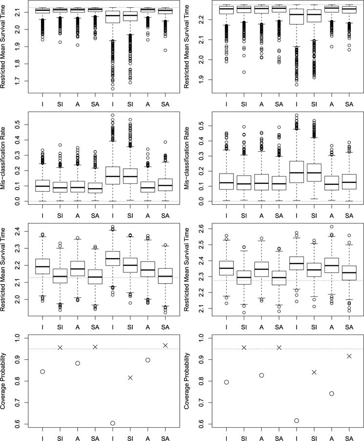
Simulation results for maximizing the RMST. The left column is for extreme value distributed error, while the right column is for logistic distributed error. The first row displays box plots for $R\left({\widehat{\eta }}^{\mathrm{opt}}\right)$, with the horizontal lines indicating the upper bound R(η^opt). The second row displays box plots for MR, with the horizontal lines indicating zero. The third row displays box plots for $\widehat{R}\left({\widehat{\eta }}^{\mathrm{opt}}\right)$, with the horizontal lines indicating the true value R(η^opt). The fourth row presents the empirical coverage probability of the confidence interval of ${\widehat{R}}_K\left({\widehat{\eta }}^{\mathrm{opt}}\right)$, with the horizontal lines indicating the nominal level of 95%. Within each panel, the left half of the plot is for correctly specified logistic regression, while right half of the plot is for misspecified logistic regression.

When the propensity score model was correctly specified, the I, SI, A, and SA approaches (the left four box plots of each panel in the first two rows) all provided good estimates of the true optimal treatment regime, that is, the simulated $R({\widehat{\eta }}^{\mathrm{opt}})$’s were very close to the upper bounds R(η^opt) and the MRs were very close to zero. When the propensity score model was mis-specified but the regression model was correctly specified (the right four box plots of each panel in the left column), the I and SI approaches had relatively large biases as expected, while the A and SA approaches still performed well, demonstrating the double robustness of the A and SA methods. When both the propensity score model and the regression model were misspecified (the right four box plots of each panel in the right column), the I, SI, A, and SA approaches all had some biases, however, the A and SA approaches had much smaller biases than those of the I and SI approaches. This implies that the augmented approaches can help to reduce the biases even when the regression model is mis-specified. In addition, as shown in the box plots given in the third row, the estimated RMST based on the unsmoothed approaches I and A all have relatively large biases, which in turn lead to empirical CP less than the nominal level. But the smoothing technique helps to reduce the biases of the estimated RMST, and thus improves the associated empirical CP. In particular, when the propensity score model was correctly specified, the SI and SA approaches have empirical CP close to 95%, while when the propensity score model was mis-specified but the regression model was correctly specified, the SA approach has correct empirical CP. The results for the median survival time were given in Figure 2. The findings for the median survival time are similar to those for the RMST.

Fig. 2.

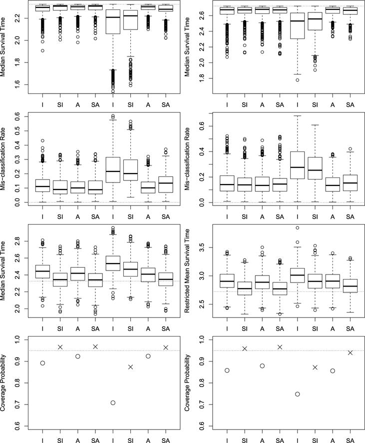
Simulation results for maximizing the median survival time. See Figure 1 for detailed descriptions of the plots.

For the simulations described above, the optimal treatment regimes obtained by maximizing the t-year survival probability, restricted mean survival time and median survival time are all the same. In this setting, the proposed methods are expected to perform similar to the method of Jiang et al. (2016) for maximizing the t-year survival probability and the method of Zhao et al. (2015) for maximizing the RMST. This is demonstrated empirically by the results in Table 1 of the Supplementary Appendix.

Additional simulations were conducted with p = 10 covariates. Specifically, the same simulation setting as above was considered, but eight additional “noise” covariates were generated independent of T, each independently generated from uniform(−2, 2). Here, we only considered the model with the extreme value distribution for the error term. For each setting, we generated 500 data sets with sample size 250. Results for the RMST and median survival time are given in Tables 2 and 3 of the Supplementary Appendix, respectively. Table entries give the true RMST and the true median survival times under the estimated optimal treatment regimes, MRs of the estimated optimal treatment regimes, and the average computation time (in seconds) per run. These results indicate that the proposed methods work reasonably well for p = 10. The estimated optimal treatment regimes for p = 10 covariates give slightly smaller values of the RMST and median survival times with nearly doubled MRs compared with the results for p = 2 covariates. This is expected because eight noise variables are added but the estimated optimal treatment regimes are not sparse. As a result, the MRs (comparing the estimated optimal regime with the true sparse regime) increased almost one-fold. On the other hand, the RMST and median survival time values of the estimated regimes only decreased slightly because the estimators of η are still close to the true value and the RMST and median survival time values of the estimated regimes are less sensitive to the biases of the estimators of η compared with the MRs. In addition, the computation time increased 1.5–5.5 times compared with simulations with p = 2 covariates.

Next, we conducted simulation studies for a setting where the regimes maximizing the median and restricted mean survival times are different. Specifically, the survival time T was generated by

$$T=12+0.5\sin (\pi (X_1-X_2))+0.25{(1+X_1+2X_2)}^2+A(0.5+2X_1-X_2)+(1+2A{X}_1^2)e,$$

where X₁ and X₂ were generated independently from uniform(−2, 2), A was generated from Bernoulli distribution with success probability 0.5 and e was an independent error generated from an exponential distribution with mean 0 and variance 1. Under this data generating mechanism, the true optimal treatment regime for maximizing the median survival time is given by η^opt = (0.760, 0.169, −0.690), which is different from the regimes that maximize the t-year survival probability and restricted mean survival time. The median survival time under the optimal treatment regime g(x; η^opt) is 14.935. The censoring time C was generated from uniform(0, C₀), where C0 was chosen to give a censoring rate of 0.25. We compare the proposed methods, the method of Jiang et al. (2016) for maximizing the t-year survival probability, the method of Zhao et al. (2015) for maximizing the RMST, and Cox regression with the linear baseline covariate effects and linear treatment-covariate interaction effects. Results based on 500 simulated data sets each with sample size 250 are summarized in Table 1. Table entries give the estimates of η, the true median survival times under the estimated optimal treatment regimens (denoted by V), and the MRs of the estimated optimal treatment regimes. Based on the results, compared with other methods, the proposed method for maximizing the estimated median survival time gives estimators of η closer to its true value, and leads to estimated optimal treatment regimes with larger median survival times and smaller MRs. Note the treatment effect is relatively small in this simulation setting, such that the advantage of the proposed method is more pronounced when comparing MR rather than V.

Table 1.

Simulation results comparing the proposed methods for maximizing the median survival time (denoted by Med) and restricted mean survival time (denoted by RM), the method of Jiang et al. (2016) (denoted by tyear), the method of Zhao et al. (2015) (denoted by Zhao) and the Cox regression (denoted by Cox). I and A denote the inverse probability weighted and augmented inverse probability weighted estimation methods, respectively; SI and SA denote the corresponding smoothing counterparts. Table entries are averages of estimates of η_j for j = 0, 1, 2, median survival times under the estimated optimal treatment regimes (V), and mis-classification rates of the estimated optimal treatment regimes (MR). The numbers in parenthesis are the standard deviations of the corresponding estimates

Method		η0	η1	η2	V	MR
Med	I	0.57 (0.32)	0.24 (0.39)	−0.54 (0.29)	14.84 (0.08)	0.20 (0.15)
Med	SI	0.58 (0.31)	0.27 (0.38)	−0.50 (0.32)	14.85 (0.07)	0.21 (0.15)
Med	A	0.59 (0.32)	0.23 (0.40)	−0.50 (0.31)	14.85 (0.07)	0.20 (0.16)
Med	SA	0.58 (0.31)	0.27 (0.39)	−0.49 (0.33)	14.85 (0.07)	0.21 (0.16)
RM	I	0.24 (0.27)	0.74 (0.16)	−0.51 (0.20)	14.79 (0.04)	0.39 (0.08)
RM	SI	0.22 (0.24)	0.78 (0.15)	−0.48 (0.19)	14.80 (0.03)	0.41 (0.07)
RM	A	0.22 (0.25)	0.77 (0.14)	−0.50 (0.18)	14.79 (0.04)	0.40 (0.07)
RM	SA	0.21 (0.22)	0.79 (0.14)	−0.48 (0.18)	14.80 (0.03)	0.41 (0.07)
tyear	I	0.29 (0.23)	0.82 (0.12)	−0.34 (0.24)	14.77 (0.06)	0.43 (0.06)
tyear	SI	0.17 (0.26)	0.86 (0.09)	−0.35 (0.18)	14.79 (0.04)	0.46 (0.04)
tyear	A	0.24 (0.27)	0.82 (0.13)	−0.33 (0.26)	14.76 (0.08)	0.45 (0.06)
tyear	SA	0.14 (0.27)	0.86 (0.11)	−0.34 (0.22)	14.77 (0.05)	0.46 (0.05)
Zhao	I	0.05 (0.55)	0.32 (0.51)	−0.26 (0.53)	14.41 (0.51)	0.45 (0.19)
Zhao	A	−0.08 (0.68)	0.15 (0.47)	−0.18 (0.51)	14.22 (0.58)	0.49 (0.23)
Cox		0.66 (0.14)	0.54 (0.15)	−0.47 (0.10)	14.81 (0.04)	0.28 (0.06)

5. Application

In this section, we apply these methods to the UNC CFAR HIV Clinical Cohort study data. Our objective is to identify the optimal treatment regime that results in the expected longest initial treatment duration. Particularly, we aim to find the optimal regime that maximizes the restricted mean initial treatment duration up to day 4000. Day 4000 is chosen so that approximately 99% of event times are less than the time point of interest. The covariates include age, gender (male vs. female), race (black, white, Hispanic, or other), MSM (yes, no, or unknown), IDU (yes, no, or unknown), CD4 count, and viral load (VL). Categorical variables are transformed into dummy variables, resulting in an 11-dimensional covariate vector X. The NNRTI plus NRTI combination is coded as treatment 1, while the PI plus NRTI combination as treatment 0. The primary outcome of interest is time to the discontinuation of the initial treatment, which is defined as either a change in the anchor agent (PI or NNRTI), or discontinuing ART for more than 30 days. Among all 990 study patients, 35% were observed to have the event of interest during follow-up, and the remaining patients were censored at their last known clinical encounter.

To estimate the optimal treatment regime, we applied the I, SI, A, and SA approaches. We first fit the logistic regression model (3) to estimate the propensity score. Table 2 shows the estimated coefficients, standard errors, and p-values of the estimates. As expected patients with lower CD4 cell counts, indicating more advanced HIV disease progression, were more likely to be prescribed a PI-based regimen, because the commonly used PI had demonstrated greater CD4 cell count recovery and less drug resistance associated with virologic failure in comparison to the commonly used NNRTI during the years of this study. Women were also more likely to be prescribed a PI-based regimen during these years because of concerns the primary NNRTI used may have had teratogenic effects [Panel on Antiretroviral Guidelines for Adults and Adolescents (2016)].

Table 2.

Estimated coefficients (Est.), standard errors (s.e.), and Wald test p-values (p-val) from the fitted logistic regression model

	Int.	age	gender male	race1 black	race2 white	race3 Hispanic	msm1 yes	msm0 no	idu1 yes	idu0 no	CD4	VL
Est.	−1.36	−0.00	0.53	−0.16	−0.59	0.15	0.11	−0.10	−0.12	0.11	0.23	0.04
s.e.	0.78	0.01	0.20	0.29	0.30	0.36	0.25	0.27	0.32	0.21	0.06	0.04
p-val	0.08	0.67	0.01	0.57	0.05	0.67	0.66	0.71	0.72	0.61	0.00	0.35

For the augmented estimation methods, we fit the proportional hazards model (5). Table 3 presents the estimated coefficients in the optimal regimes obtained by the I, SI, A, and SA approaches. Overall, the four estimated optimal treatment regimes give relatively similar treatment allocation rules. Here, we examine the results using the regime $g(x;{\widehat{\eta }}_{\mathit{SA}}^{\mathrm{opt}})$ obtained by the SA approach. We estimate the restricted mean survival times under the estimated optimal regimes and compare these restricted mean survival times with those under the fixed treatment regimes by assigning all patients to one treatment. The restricted mean survival time is 2776 days under the regime $g({\widehat{\eta }}_{\mathit{SA}}^{\mathrm{opt}})$, 2637 days if all the patients were given treatment 1, and 2339 days if all the patients were given treatment 0. Figure 3 shows the estimated survival curves under the regime $g({\widehat{\eta }}_{\mathit{SA}}^{\mathrm{opt}})$, the fixed regimes, and the observed treatment assignment (i.e., the empirical regime). The estimated survival curve under the estimated optimal treatment regime $g({\widehat{\eta }}_{\mathit{SA}}^{\mathrm{opt}})$ is uniformly better than under the empirical and fixed regimes, indicating that the estimated optimal individualized treatment regime may lead to improved clinical outcomes if used in routine medical care. Additionally, the estimated survival curve if all patients were assigned to treatment 1 led to better patient outcomes than if all patients were assigned to treatment 0. Given the antiretroviral agents used in these calendar years these findings are not surprising. The NNRTI used as an anchor agent for treatment 1 continues to be recommended for initial HIV treatment; however, with one exception the PIs included in treatment 0 are no longer recommended as initial treatment [Gunthard et al. (2014)]. Table 4 shows the 95% confidence intervals of the difference between the restricted mean survival times under the estimated optimal regimes obtained by the I, A, SI, and SA approaches and the fixed regimes. The estimated optimal treatment regimes significantly increase the restricted mean survival times of the initial treatment duration compared with the fixed treatment regimes.

Table 3.

Estimated coefficients of optimal treatment regimes by the I, SI, A, and SA methods

	int.	age	gender	race1	race2	race3	msm1	msm0	idu1	idu0	CD4	VL
I	0.38	−0.02	−0.26	−0.15	−0.53	−0.58	−0.16	−0.13	−0.23	−0.18	0.11	0.09
SI	0.48	−0.02	−0.12	0.13	−0.35	−0.46	−0.09	−0.10	−0.43	−0.44	0.03	0.09
A	0.25	−0.01	0.54	−0.36	−0.39	−0.17	−0.26	0.10	0.38	0.08	−0.26	0.21
SA	0.48	−0.02	−0.09	0.07	−0.36	−0.47	−0.10	−0.08	−0.43	−0.44	0.03	0.09

Fig. 3.

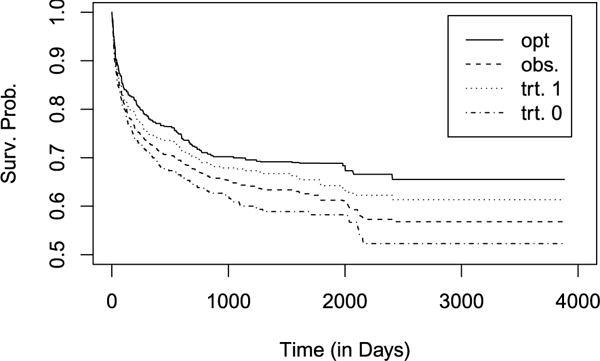
Survival function estimates if all the patients followed $g(x;{\widehat{\eta }}_{\mathit{SA}}^{\mathrm{opt}})$ (solid line), the observed treatment (dashed line), received treatment 1 (dotted line) or received treatment 0 (dotted dashed line).

Table 4.

Confidence intervals for the difference of estimated restricted mean survival times

	compared to trt. 1	compared to trt. 0
I	(63, 286)	(232, 707)
SI	(54, 249)	(199, 694)
A	(20, 139)	(123, 631)
SA	(47, 231)	(189, 684)

Next, we compare treatment allocation of the observed treatment assignment and the estimated optimal regime $g(x;{\widehat{\eta }}_{\mathit{SA}}^{\mathrm{opt}})$ in Table 5. Overall only 55% of the patients received the ART estimated to be the optimal ART by the SA approach. Moreover, the SA approach estimated that 85% patients who received a PI should have received an NNRTI, but only 14% of patients who received an NNRTI would have fared better if they had received a PI-based ART. These findings are supported by the estimated survival curves given in Figure 3 since the survival function if the whole population received treatment 1 is uniformly better than if all patients received treatment 0.

Table 5.

Comparison between the observed treatment assignment and recommended treatment by the regime $g({\widehat{\eta }}_{\mathit{SA}}^{\mathrm{opt}})$

		A
		0	1
$g({\widehat{\eta }}_{\mathit{SA}}^{\mathrm{opt}})$	0	63	76
	1	367	484

We also compare treatment allocation of the empirical regime and the estimated optimal regime $g(x;{\widehat{\eta }}_{\mathit{SA}}^{\mathrm{opt}})$ across strata of each demographic and clinical patient characteristic of interest. Figures 4 and 5 present the results for the categorical and continuous covariates, respectively. For continuous covariates age, CD4 count, and VL, we discretized them into four ranges based on quartiles. Consistent with observations for the entire study population (Figure 3), the estimated optimal regime overwhelmingly favored initiating an NNRTI-based ART versus a PI-based ART across all patient characteristics. In nearly all cases, a greater proportion of patients were allocated to treatment 1 (an NNRTI) by the estimated optimal regime than were observed to receive treatment 1. During the years of this study, the PI used most frequently, in comparison to the predominantly used NNRTI, had slightly lower efficacy in reducing circulating HIV RNA levels, but was associated with slightly greater CD4 cell count recovery and lower antiretroviral drug resistance evolution with virologic failure [Panel on Antiretroviral Guidelines for Adults and Adolescents (2016)]. These known properties of the primary anchor agents available at the time, in addition to slightly different tolerability profiles of the antiretrovirals under consideration, likely influenced the channeling bias observed in clinical care and shaped the estimated optimal regime results. For example, this effect can be observed for CD4 cell count (Figure 5) where it is clear that patients with lower CD4 were more likely to be prescribed a PI-based ART than those at higher CD4 cell counts. A further example is age, in general patients at older ages enter HIV care and start ART at lower CD4 where a PI-based ART may have been more effective. In general, men entered HIV care, and hence started ART, at lower CD4 cell counts in this clinical cohort, therefore, as expected the estimated optimal regime was PI-based in a greater proportion of men than women (Figure 4). On the other hand a PI-based regime was prescribed to women at a higher proportion than men. In part, this may be related to the efficacy and tolerability differences in the agents used, as described above. Additionally, there were clinical concerns that the primary NNRTI available at the time had teratogenic effects and, therefore, women of reproductive age may have been steered away from NNRTI use.

Fig. 4.

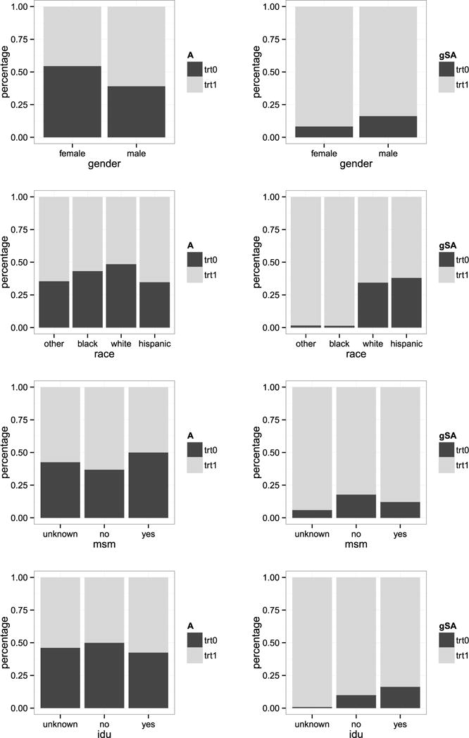
Comparison of treatment allocation percentages stratified on each categorical covariates. The left panel is for the observed assignment while the right panel is for the estimated optimal treatment regime (denoted by gSA).

Fig. 5.

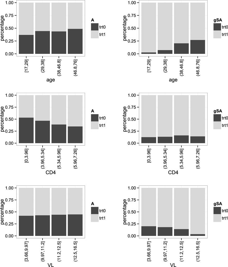
Comparison of treatment allocation percentages stratified on each continuous covariates (based on quartiles). The left panel is for the observed assignment while the right panel is for the estimated optimal treatment regime (denoted by gSA).

6. Extension

6.1. Framework

In this section, we extend the proposed methods from Section 3 to multi-stage studies, where treatment assignment is made at multiple time points based on patients’ covariate information available at each time point. For simplicity, we consider a two-stage study, with two treatment options at each stage. Assume treatment A₁ is assigned s days after the initial treatment A₀. The objective is still to maximize either the RMST up to time L or the median survival time.

For each patient, baseline covariates X₀ are collected at the first visit and the initial treatment $A_0\in {\mathcal{A}}_0=\left\{0,1\right\}$ is assigned based on X₀. The follow-up visit is scheduled at s days after the initial visit. If the patient is still at risk at the second visit, additional covariates X₁ are collected and the follow-up treatment $A_1\in {\mathcal{A}}_1=\left\{0,1\right\}$ is given based on the accumulated information X₀, A₀ and X₁. Thus, the observed data is $\left\{(X_{0i},A_{0i},X_{1i}I\left\{{\stackrel{\sim }{T}}_i>s\right\},A_{1i}I\left\{{\stackrel{\sim }{T}}_i>s\right\},{\stackrel{\sim }{T}}_i,{\delta }_i),i=1,\dots ,n\right\}$.

6.2. Methods

We want to find the optimal dynamic regime g = (g₀, g₁) which maximizes the restricted mean survival time or median survival time, respectively. As before, we consider regimes of the form

$$g_0\left(x_0;{\eta }_0\right)=I\left\{{\eta }_0^T\left(1,x_0^T\right)\ge 0\right\},$$

$$g_1\left(x_0,x_1;{\eta }_1\right)=I\left\{{\eta }_1^T\left(1,x_0^T,g_0\left(x_0;{\eta }_0\right),x_1^T\right)\ge 0\right\}.$$

Equation (1) is still applicable in the multi-stage studies, if the weight function is replaced with

$$w^{\left(2\right)}=\frac{I\left({\stackrel{\sim }{T}}_i\le s\right){\delta }_i}{{\widehat{S}}_C\left({\stackrel{\sim }{T}}_i\right)}\times \frac{I\left\{A_{0i}=g_0\left(X_{0i};{\eta }_0\right)\right\}}{{\widehat{\pi }}_{A_0}\left(X_{0i}\right)}+\frac{I\left({\stackrel{\sim }{T}}_i>s\right)}{{\widehat{S}}_C\left(s\right)}\times \frac{I\left\{A_{0i}=g_0\left(X_{0i};{\eta }_0\right),A_{1i}=g_1\left(X_{0i},X_{1i};{\eta }_0\right)\right\}}{{\widehat{\pi }}_{A_0}\left(X_{0i}\right){\widehat{\pi }}_{A_1}\left(X_{0i},A_{0i},X_{1i}\right)},$$

where ${\widehat{\pi }}_{A_0}\left(X_{0i}\right)={\widehat{\pi }}_0\left(X_{0i}\right)A_{0i}+\left\{1-{\widehat{\pi }}_0\left(X_{0i}\right)\right\}\left(1-A_{0i}\right)$, ${\widehat{\pi }}_{A_1}\left(X_{0i},A_{0i},X_{1i}\right)={\widehat{\pi }}_1\left(X_{0i},A_{0i},X_{1i}\right)A_{1i}+\left\{1-{\widehat{\pi }}_1\left(X_{0i},A_{0i},X_{1i}\right)\right\}\left(1-A_{1i}\right)$ and ${\widehat{\pi }}_0\left(X_{0i}\right)$ and ${\widehat{\pi }}_1\left(X_{0i},A_{0i},X_{1i}\right)$ are the maximum likelihood estimates of the propensity scores P (A_0i = 1|X_0i) and $P(A_{1i}=1|X_{0i},A_{0i},X_{1i},{\stackrel{\sim }{T}}_i>s)$, respectively. See Jiang et al. (2016) for details. Let ${\widehat{S}}_I^{(2)}\left(u,\eta \right)$ denote the resulting estimator of the survival function S⁽²⁾(u, η) under the regime g(x₀, x₁; η).

We can also apply the kernel smoothing technique to improve finite sample performance in the multi-stage setting. Specifically, we replace the indicator functions g₀ (X_0i; η₀) and g₁(X_0i, X_1i; η₁) in ${\widehat{S}}_I^{(2)}\left(u,\eta \right)$ by $\mathrm{\Phi }\left({\eta }_0^T\left(1,X_{0i}^T\right)/h_0\right)$ and $\mathrm{\Phi }\left({\eta }_1^T\left(1,X_{0i}^T,g_0\left(X_{0i};{\eta }_0\right),X_{1i}^T\right)/h_1\right)$, respectively, where h₀ and h₁ are bandwidths. The resulting smoothed estimator is denoted by ${\widehat{S}}_{SI}^{(2)}\left(u;\eta \right)$. A natural estimator of the optimal dynamic treatment regime is given by ${\widehat{g}}_{\eta }^{\mathrm{opt},\left(2\right)}=\left\{g_0\left(X_0;{\widehat{\eta }}_{K,0}^{\mathrm{opt},\left(2\right)}\right),g_1\left(X_0,X_1;{\widehat{\eta }}_{K,0}^{\mathrm{opt},\left(2\right)}\right)\right\}$ where ${\widehat{\eta }}_K^{\mathrm{opt},\left(2\right)}=\left({\widehat{\eta }}_{K,0}^{\mathrm{opt},\left(2\right)},{\widehat{\eta }}_{K,1}^{\mathrm{opt},\left(2\right)}\right)$ maximizes $f\left({\widehat{S}}_K^{\left(2\right)}\left(t;\eta \right)\right)$, k = I or SI, and f is a user-specified function, such as the RMST or median survival time.

Let ${\widehat{R}}_K^{\left(2\right)}\left({\widehat{\eta }}_K^{\mathrm{opt},\left(2\right)}\right)$ and ${\widehat{\xi }}_K^{\left(2\right)}\left({\widehat{\eta }}_K^{\mathrm{opt},\left(2\right)}\right)$ denote the estimated RMST and median survival time under the estimated optimal dynamic treatment regime ${\widehat{g}}_{\eta }^{\mathrm{opt},\left(2\right)}$, respectively. Jiang et al. (2016) showed that ${\widehat{S}}_K^{(2)}\left(u,\eta \right)$ is a consistent estimator for S⁽²⁾(u, η) no matter whether u ≥ s or u < s. Following the proof in Jiang et al. (2016), it can be shown that the estimators ${\widehat{R}}_K^{\left(2\right)}\left({\widehat{\eta }}_K^{\mathrm{opt},\left(2\right)}\right)$ and ${\widehat{\xi }}_K^{\left(2\right)}\left({\widehat{\eta }}_K^{\mathrm{opt},\left(2\right)}\right)$ are consistent and asymptotically normal. Theorem 3 establishes the asymptotic properties of these estimators.

Theorem 3

Under certain regularity conditions (see the Supplementary Appendix), when model ${\pi }_{A_0}$ and ${\pi }_{A_1}$ are correctly specified, as n → ∞:

1. ${\widehat{R}}_K^{\left(2\right)}\left({\widehat{\eta }}_K^{\mathrm{opt},\left(2\right)}\right)$ is consistent for R⁽²⁾(η^opt,(2)) and $\sqrt{n}\left\{{\widehat{R}}_K^{\left(2\right)}\left({\widehat{\eta }}_K^{\mathrm{opt},\left(2\right)}\right)-R^{\left(2\right)}\left({\eta }^{\mathrm{opt},\left(2\right)}\right)\right\}{\to }^{d}N\left\{0,{\sigma }_{R,K}^2\left({\eta }^{\mathrm{opt},\left(2\right)}\right)\right\}$, for K = I or SI.

2. ${\widehat{\xi }}_K^{\left(2\right)}\left({\widehat{\eta }}_K^{\mathrm{opt},\left(2\right)}\right)$ is consistent for ξ⁽²⁾(η^opt,(2)) and $\sqrt{n}\left\{{\widehat{\xi }}_K^{\left(2\right)}\left({\widehat{\eta }}_K^{\mathrm{opt},\left(2\right)}\right)-{\xi }^{\left(2\right)}\left({\eta }^{\mathrm{opt},\left(2\right)}\right)\right\}{\to }^{d}N\left\{0,{\sigma }_{\xi ,K}^2\left({\eta }^{\mathrm{opt},\left(2\right)}\right)\right\}$, for K = I or SI.

As before, smoothing does not impact the asymptotic distribution. In addition, the asymptotic variances of the estimators can be consistently estimated in a similar fashion as for the one-stage estimators. We conducted simulation studies to investigate the finite sample properties of the proposed two-stage estimators. The simulation settings and results are given in the s. Both I and SI based methods performed well and again smoothing helped improve the finite sample performance.

7. Discussion

In this paper, we proposed a doubly robust estimation method for obtaining the optimal treatment regime which maximizes a prespecified function of the survival function, including the RMST and median survival time as special cases. The proposed method can be employed to determine optimal individualized treatment regimes that balance short-term and long-term treatment effects on survival, thus providing optimal regimens that target clinically meaningful quantities of interest. Extensions to multistage studies were also developed, broadening the scope of settings where this method can be applied.

There are several possible avenues of future related research. For instance, in survival analysis it is common for competing risks to be present. In the HIV context, the initial treatment may be discontinued due to several competing reasons. Thus it would be of interest to extend the proposed method to incorporate competing risks. One approach could entail deriving nonparametric estimators of the cumulative incidence function associated with a given treatment regime and then determining the optimal treatment regime which maximizes a pre-specified function of the cumulative incidence function. Another common occurrence in survival analysis, especially in HIV studies, is interval censoring wherein the failure time is known only to occur within some interval. Extensions of the proposed methods to allow for interval censoring is another possible area of future research. Finally, similar to the value search method of Jiang et al. (2016), the proposed methods directly maximize the estimated RMST or median survival time using a genetic algorithm. A computational limitation of such algorithms is the inability to handle high-dimensional covariates. Thus extensions of the proposed method to allow for high-dimensional covariates could also be considered.

APPENDIX

Proof of Theorem 1

As shown in Jiang et al. (2016), for any time point t < τ, ${\widehat{S}}_K\left(t;{\widehat{\eta }}_K^{\mathrm{opt}}\right)$ is consistent for S(t; η^opt) and

$$\sqrt{n}\left\{{\widehat{S}}_K\left(t;{\widehat{\eta }}_K^{\mathrm{opt}}\right)-S\left(t;{\eta }^{\mathrm{opt}}\right)\right\}=\frac{1}{\sqrt{n}}{\displaystyle \sum _{i=1}^n{\zeta }_{i,K}\left(t;{\eta }^{\mathrm{opt}},{\alpha }^{\ast }\right)}+o_p\left(1\right),$$

where ζ_i,K(t; η, α^∗) is the ith influence function for ${\widehat{S}}_K\left(t;\eta ,\widehat{\alpha }\right)$ and α* includes all parameters the treatment assignment model and/or the regression model. For any pre-determined time point L, the RMST up to L is a continuous function of S(t; η). By applying the continuous mapping theorem, ${\widehat{R}}_K\left({\widehat{\eta }}^{\mathrm{opt}}\right)$ is consistent for R(η^opt).

By applying the delta method, we have

$$\sqrt{n}\left\{{\widehat{R}}_K\left({\widehat{\eta }}_K^{\mathrm{opt}},\widehat{\alpha }\right)-R\left({\eta }^{\mathrm{opt}}\right)\right\}=\frac{1}{\sqrt{n}}{\displaystyle \sum _{i=1}^n{\rho }_{i,K}\left({\eta }^{\mathrm{opt}},{\alpha }^{\ast }\right)}+o_p\left(1\right)$$

where

$${\rho }_{i,K}\left({\eta }^{\mathrm{opt}},{\alpha }^{\ast }\right)=-{\displaystyle {\int }_0^{L}S\left(t;{\eta }^{\mathrm{opt}}\right){\zeta }_{i,K}\left(t;{\eta }^{\mathrm{opt}},{\alpha }^{\ast }\right)dt}.$$

Thus, ${\widehat{R}}_K\left({\widehat{\eta }}_K^{\mathrm{opt}},\widehat{\alpha }\right)$ is asymptotic normal with variance ${\sigma }_{R,K}^2\left({\eta }^{\mathrm{opt}}\right)=E\left[{\left\{{\rho }_{i,K}\left({\eta }^{\mathrm{opt}},{\alpha }^{\ast }\right)\right\}}^2\right]$, which can be consistently estimated by

$${\widehat{\sigma }}_{R,K}^2\left({\widehat{\eta }}^{\mathrm{opt}}\right)=n^{-1}{\displaystyle \sum _{i=1}^n{\left[{\displaystyle {\int }_0^L{\widehat{S}}_K\left(t;{\widehat{\eta }}_K^{\mathrm{opt}}\right){\zeta }_{i,K}\left(t;{\widehat{\eta }}_K^{\mathrm{opt}},\widehat{\alpha }\right)dt}\right]}^2}.$$

Proof of Theorem 2

Recall that median survival time is also a continuous function of survival time. Define ϕ(S(t; η)) = S⁻¹(0.5; η) = inf {t : S(t η) ≥ 0.5}. We have ξ(η) = ϕ(S(t; η)) and ${\widehat{\xi }}_K\left({\widehat{\eta }}_K^{\mathrm{opt}}\right)=\varphi \left({\widehat{S}}_K\left(t;{\widehat{\eta }}_K^{\mathrm{opt}}\right)\right)$. Applying the continuous mapping theorem, ${\widehat{\xi }}_K\left({\widehat{\eta }}_K^{\mathrm{opt}}\right)$ can be shown to be consistent for ξ(η^opt).

To derive the limiting distribution of ${\widehat{\xi }}_K\left({\widehat{\eta }}_K^{\mathrm{opt}}\right)$, we follow the steps in Gill, Keiding and Andersen (1997), Section IV.3.4. When regularity condition A10 holds, ϕ is compactly differentiable at S. We have

$$\sqrt{n}\left\{{\widehat{\xi }}_K\left({\widehat{\eta }}_K^{\mathrm{opt}}\right)-\xi \left({\eta }^{\mathrm{opt}}\right)\right\}=\frac{1}{q\left(\xi ;{\eta }^{\mathrm{opt}}\right)}\sqrt{n}\left\{{\widehat{S}}_K\left(\xi ;{\widehat{\eta }}_K^{\mathrm{opt}}\right)-S\left(\xi ;{\eta }^{\mathrm{opt}}\right)\right\}+o_p\left(1\right).$$

Thus,

$$\sqrt{n}\left\{{\widehat{\xi }}_K\left({\widehat{\eta }}_K^{\mathrm{opt}}\right)-\xi \left({\eta }^{\mathrm{opt}}\right)\right\}\stackrel{d}{\to }N\left(0,\frac{{\sigma }_K^2\left(\xi ;{\eta }^{\mathrm{opt}}\right)}{q^2\left(\xi ;{\eta }^{\mathrm{opt}}\right)}\right),$$

where ${\sigma }_K^2\left(\xi ;{\eta }^{\mathrm{opt}}\right)$ is the asymptotic variance of the estimator ${\widehat{S}}_K\left(\xi ;{\widehat{\eta }}_K^{\mathrm{opt}}\right)$ as derived in Jiang et al. (2016). A consistent estimator of ${\sigma }_{\xi ,K}^2\left({\eta }^{\mathrm{opt}}\right)={\sigma }_K^2\left(\xi ;{\eta }^{\mathrm{opt}}\right)/q^2\left(\xi ;{\eta }^{\mathrm{opt}}\right)$ can be obtained as ${\widehat{\sigma }}_K^2\left({\widehat{\xi }}_K\left({\widehat{\eta }}_K^{\mathrm{opt}}\right);{\widehat{\eta }}_K^{\mathrm{opt}}\right)/\widehat{q}\left({\widehat{\xi }}_K\left({\widehat{\eta }}_K^{\mathrm{opt}}\right);{\widehat{\eta }}_K^{\mathrm{opt}}\right)$, where

$$\widehat{q}\left(v;\eta \right)=-\frac{1}{h}{\displaystyle {\int }_0^{\infty }\phi \left(\frac{v-u}{h}\right)d{\widehat{S}}_K\left(u;\eta \right)},$$

φ(x) is the density function for the standard normal distribution and $h=sd\left({\stackrel{\sim }{T}}_i\right)\ast n^{-1/5}$ is the bandwidth.

Proof of Theorem 3

The proof of Theorem 3 is similar to those of Theorems 1 and 2, and is omitted here.

References

- Bai X, Tsiatis AA, O’Brien SM. Doubly-robust estimators of treatment-specific survival distributions in observational studies with stratified sampling. Biometrics. 2013;69:830–839. doi: 10.1111/biom.12076. MR3146779. [DOI] [PMC free article] [PubMed] [Google Scholar]
- Chen PY, Tsiatis AA. Causal inference on the difference of the restricted mean lifetime between two groups. Biometrics. 2001;57:1030–1038. doi: 10.1111/j.0006-341x.2001.01030.x. MR1950418. [DOI] [PubMed] [Google Scholar]
- Cox DR. Regression models and life-tables. J Roy Statist Soc Ser B. 1972;34:187–220. MR0341758. [Google Scholar]
- Dombrowski JC, Kitahata MM, Rompaey SEV, Crane HM, Mugavero MJ, Eron JJ, Boswell SL, Rodriguez B, Mathews WC, Martin JN, Moore RD, Golden MR. High levels of antiretroviral use and viral suppression among persons in HIV care in the United States, 2010. J Acquir Immune Defic Syndr. 2013;63:299–306. doi: 10.1097/QAI.0b013e3182945bc7. [DOI] [PMC free article] [PubMed] [Google Scholar]
- Gill RD, Keiding N, Andersen PK. Statistical Models Based on Counting Processes. Springer; New York: 1997. [Google Scholar]
- Goldberg Y, Kosorok MR. Q-learning with censored data. Ann Statist. 2012;40:529–560. doi: 10.1214/12-AOS968. MR3014316. [DOI] [PMC free article] [PubMed] [Google Scholar]
- Gunthard HF, Aberg JA, Eron JJ, Hoy JF, Telenti A, Benson CA, Burger DM, Cahn P, Gallant JE, Glesby MJ, Reiss P, Saag MS, Thomas DL, Jacobsen DM, Volberding PA. Antiretroviral treatment of adult HIV infection: 2014 recommendations of the International Antiviral Society-USA panel. JAMA J Am Med Assoc. 2014;312:410–425. doi: 10.1001/jama.2014.8722. [DOI] [PubMed] [Google Scholar]
- Howe CJ, Cole SR, Napravnik S, Eron JJ., JR Enrollment, retention, and visit attendance in the University of North Carolina Center for AIDS Research Clinical Cohort, 2001–2007. AIDS Res Hum Retrovir. 2010;26:875–881. doi: 10.1089/aid.2009.0282. [DOI] [PMC free article] [PubMed] [Google Scholar]
- Irwin JO. The standard error of an estimate of expectation of life, with special reference to expectation of tumourless life in experiments with mice. J Hyg. 1949;47:188–189. doi: 10.1017/s0022172400014443. [DOI] [PMC free article] [PubMed] [Google Scholar]
- Jiang R, Lu W, Song R, Davidian M. On estimation of optimal treatment regimes for maximizing t-year survival probability. J R Stat Soc Ser B Stat Methodol. 2016 doi: 10.1111/rssb.12201. To appear. [DOI] [PMC free article] [PubMed] [Google Scholar]
- Jiang R, Lu W, Song R, Hudgens MG, Naprvavnik S. Supplement to “Doubly robust estimation of optimal treatment regimes for survival data—with application to an HIV/AIDS study”. 2017 doi: 10.1214/17-AOAS1057SUPP. [DOI] [PMC free article] [PubMed] [Google Scholar]
- Kaplan EL, Meier P. Nonparametric estimation from incomplete observations. J Amer Statist Assoc. 1958;53:457–481. MR0093867. [Google Scholar]
- Mebane WR, Jr, Sekhon JS. Genetic optimization using derivatives: The rgenoud package for R. J Stat Softw. 2011;42:1–26. [Google Scholar]
- Murphy SA. Optimal dynamic treatment regimes. J R Stat Soc Ser B Stat Methodol. 2003;65:331–366. MR1983752. [Google Scholar]
- Murphy SA. A generalization error for Q-learning. J Mach Learn Res. 2005;6:1073–1097. MR2249849. [PMC free article] [PubMed] [Google Scholar]
- Panel on Antiretroviral Guidelines for Adults and Adolescents. Guidelines for the use of antiretroviral agents in HIV-1-infected adults and adolescents. Department of Health and Human Services; 2016. Available at: https://aidsinfo.nih.gov/contentfiles/lvguidelines/adultandadolescentgl.pdf. [Google Scholar]
- Robins JM. Proceedings of the Second Seattle Symposium in Biostatistics. Lect Notes Stat. Vol. 179. Springer; New York: 2004. Optimal structural nested models for optimal sequential decisions; pp. 189–326. MR2129402. [Google Scholar]
- Tian L, Alizadeh AA, Gentles AJ, Tibshirani R. A simple method for estimating interactions between a treatment and a large number of covariates. J Amer Statist Assoc. 2014;109:1517–1532. doi: 10.1080/01621459.2014.951443. MR3293607. [DOI] [PMC free article] [PubMed] [Google Scholar]
- Watkins CJCH, Dayan P. Q-learning. Mach Learn. 1992;8:279–292. [Google Scholar]
- Willig JH, Abroms S, Westfall AO, Routman J, Adusumilli S, Varshney M, Allison J, Chatham A, Raper JL, Kaslow RA, Saag MS, Mugavero MJ. Increased regimen durability in the era of once daily fixed-dose combination antiretroviral therapy. AIDS. 2008;22:1951–1960. doi: 10.1097/QAD.0b013e32830efd79. [DOI] [PMC free article] [PubMed] [Google Scholar]
- Zhao Y, Kosorok MR, Zeng D. Reinforcement learning design for cancer clinical trials. Stat Med. 2009;28:3294–3315. doi: 10.1002/sim.3720. MR2750277. [DOI] [PMC free article] [PubMed] [Google Scholar]
- Zhao YQ, Zeng D, Laber EB, Song R, Yuan M, Kosorok MR. Doubly robust learning for estimating individualized treatment with censored data. Biometrika. 2015;102:151–168. doi: 10.1093/biomet/asu050. MR3335102. [DOI] [PMC free article] [PubMed] [Google Scholar]
- Zucker DM. Restricted mean life with covariates: Modification and extension of a useful survival analysis method. J Amer Statist Assoc. 1998;93:702–709. MR1631365. [Google Scholar]
Associated Data
This section collects any data citations, data availability statements, or supplementary materials included in this article.