Nonlinear Imaging of Microbubble Contrast Agent Using the Volterra Filter: In Vivo Results

Abstract

A nonlinear filtering approach to imaging the dynamics of microbubble ultrasound contrast agents (UCA) in microvessels is presented. The approach is based on the adaptive third-order Volterra filter (TVF), which separates the linear, quadratic, and cubic components from beamformed pulse-echo ultrasound data. The TVF captures polynomial nonlinearities utilizing the full spectral components of the echo data and not from prespecified bands, e.g. second or third harmonics. This allows for imaging using broadband pulse transmission to preserve the axial resolution and the SNR. In this paper, we present results from imaging the UCA activity in a 200-µm cellulose tube embedded in a tissue-mimicking phantom using a linear array diagnostic probe. The contrast enhancement was quantified by computing the contrast-to-tissue ratio (CTR) for the different imaging components, i.e. B-mode, pulse inversion (PI), and the TVF components. The temporal mean and standard deviation of the CTR values were computed for all frames in a given data set. Quadratic and cubic images, referred to as QB-mode and CB-mode, produced higher mean CTR values than B-mode, which showed improved sensitivity. Compared to PI, they produced similar or higher mean CTR values with greater spatial specificity. We also report in vivo results from imaging UCA activity in an implanted LNCaP tumor with heterogeneous perfusion. The temporal means and standard deviations of the echogenicity were evaluated in small regions with different perfusion levels in the presence and absence of UCA. The in vivo measurements behaved consistently with the corresponding calculations obtained under microflow conditions in vitro. Specifically, the nonlinear VF components produced larger increases in the temporal mean and standard deviation values compared to B-mode in regions with low to relatively high perfusion. These results showed that polynomial filters such as the TVF can provide an important tool for imaging UCA activity in regions with heterogeneous perfusion as is the case in some tumors and ischemic tissues.

I. Introduction

MICROBUBBLE ultrasound contrast agents (UCA) continue to offer significant promises in a variety of diagnostic and therapeutic applications [1]–[6]. Perfusion imaging is a major diagnostic application of UCA where the nonlinear response of the microbubbles plays an important role in determining the sensitivity and the specificity. The dominant nature of the echoes from the surrounding tissue relative to the UCA echo components represents a major challenge for realizing high-specificity perfusion imaging. It was realized early on that the standard B-mode imaging does not have the sensitivity to image perfusion [7].

Several harmonic imaging methods exploiting the nonlinear oscillations of microbubbles, together with the use of low mechanical index (MI) to minimize tissue nonlinearity, have been developed [8]–[10].

Haider et al [11] proposed to use higher harmonic components to improve SNR and preserve tissue information, but only odd orders showed better performance, due to spectral folding. Amplitude modulation was proposed in [12] and extended to phase and amplitude modulation [11]. Later, a combined pulse inversion and amplitude modulation (PIAM) was proposed in [13] to increase the SNR and sensitivity to UCA activities. The sensitivity improvement for even order components has been stressed [11], [13]. However, PIAM approaches, including the pulse inversion (PI) method [14], require multipulse transmission for acquisition of each image line, which results in reducing the frame rate.

The PI method has been extended to incorporate Doppler processing through the use of multiple inverted pulses [14]. More recently, the PI Doppler method has been demonstrated using high-speed plane-wave imaging [15]. This approach enables the simultaneous imaging of perfusion and flow, which addresses an important clinical limitation of previously proposed UCA perfusion imaging methods.

We have introduced the concept of post-beamforming nonlinear filtering of ultrasound echo data for separating the linear and nonlinear components using the Volterra filter (VF) [16]. This can be achieved without the need for multipulse transmissions, which addresses the motion sensitivity problem. At the same time, like the multipulse methods, it does not require bandlimiting the transmit pulses to simplify the separation of the linear and nonlinear components. That is, the VF can be designed to extract nonlinear echo components (e.g. quadratic, cubic, etc.) throughout the spectrum of the echo data, not just at the expected bands (e.g. 2nd harmonic, subharmonics, or ultraharmonics). This allows for the use of standard imaging pulses designed to provide the best possible resolution and SNR in the fundamental (B-)mode by utilizing the full bandwidth of the imaging probe. We have described the various implementations of the VF in its 2nd order [16] and 3rd order [17] and compared its performance to pulse inversion [18] both in vitro and in vivo [19]. Most recently, we have developed an adaptive third-order VF and described its performance in terms of the spectral and statistical characteristics of the echo data and its linear and nonlinear components [20], [21].

In this paper, we provide a full description of the theory and implementation of our adaptive third-order VF for separating the linear, quadratic and cubic components of ultrasound echo data. We illustrate its performance with experimental data acquired from imaging microflow of UCA solution in a 200-µm cellulose channel embedded in a tissue-mimicking phantom. Comparisons with B-mode and pulse inversion are given in terms of the spatial specificity and contrast-to-tissue ratio (CTR). The spectra of the VF filter components (i.e. linear, quadratic and cubic) in UCA and tissue regions are also given to illustrate the broadband nature of UCA enhancement under microflow conditions. Results from in vivo imaging of heterogeneous perfusion in a LNCap tumor are reported. The results show that the UCA enhancements in vivo are consistent with the in vitro microflow results.

II. Theory

A. Adaptive Third-order Volterra Filter

The Volterra filter is one of the most commonly used nonlinear filters [22], [23]. It is a polynomial filter with memory, which can be finite or infinite. The discrete third-order VF, for example, can be implemented by the following finite-memory difference equation:

$$\widehat{x}\left[n+1\right]=\nu \left[n\right]+{\displaystyle \sum _{i=0}^{m-1}x\left[n-i\right]}{h}_L\left[i\right]+{\displaystyle \sum _{i=0}^{m-1}{\displaystyle \sum _{j=0}^{m-1}x\left[n-i\right]x\left[n-j\right]h_Q\left[i,j\right]}}+{\displaystyle \sum _{i=0}^{m-1}{\displaystyle \sum _{j=0}^{m-1}{\displaystyle \sum _{k=0}^{m-1}x\left[n-i\right]x\left[n-j\right]x\left[n-k\right]h_C\left[i,j,k\right]}}}=\nu \left[n\right]+x_L\left[n\right]+x_Q\left[n\right]+x_C\left[n\right],$$ (1)

where x[n] is the input signal, e.g. beamformed RF data in pulse-echo ultrasound. The kernels, h_L[n], h_Q[n₁, n₂] and h_C[n₁, n₂, n₃], operate on the polynomial products of the input data x[n] to extract the linear, quadratic and cubic components, respectively. The output signals represent the linear, x_L[n], quadratic, x_Q[n], cubic, x_C[n] and residual, ν[n]. The residual component accounts for noise and higher-order nonlinearities which are not accounted for by the filter. The signal decomposition operation of the TVF is schematically represented in Figure 1.

Fig. 1.

A schematic representation of signal decomposition using a TVF.

The TVF decomposition shown in (1) offers several advantages in signal processing. First, it can be implemented readily in much the same manner as a finite-impulse response (FIR) filter. In fact, the linear component, x_L, is the standard convolution with a 1D FIR filter kernel of length m. The higher order components, represent a special form of “polynomial” convolution that extract quadratic (using h_Q) and cubic (using h_C) interactions with memory, m − 1. Second, the 2nd and 3rd order filtering operations, producing x_Q and x_C, have been shown to completely reject additive Gaussian noise [24], [25], which is beneficial in ultrasound imaging, especially in low MI imaging. Third, and perhaps most importantly, the quadratic and cubic kernels, when appropriately matched to the signal nonlinearities, capture quadratic and cubic interactions throughout the full observable frequency range, not just in specific bands such as the second and third harmonics.

B. Determination of the Volterra Filter Kernel Coefficients

Equation 1 provides a means for determining the values of the TVF kernel coefficients through a minimum norm least square (MNLS) solution as suggested in [16], [17]. This is based on the fact that, while (1) is nonlinear in the data, it is linear with respect to the kernel coefficients. Therefore, it is possible to form an equation of the form,

$${\mathit{G}}_n{\mathit{h}}_n={\mathit{x}}_n+{\mathit{\nu }}_n$$ (2)

where

$${\mathit{h}}_n=[h_L\left[0\right],h_L\left[1\right],\dots ,h_L\left[m-1\right],\dots h_Q\left[0,0\right],\dots ,h_Q\left[m-1,m-1\right],\dots {h_C\left[0,0,0\right],\dots ,h_C\left[m-1,m-1,m-1\right]]}^T$$

is the unknown vector containing the linear, quadratic and cubic kernel coefficients. The vector x_n represents the observed data at N samples x_n = [x[n], x[n − 1],⋯, x[n − N + 1]]^T. The data matrix G_n is given by

$${\mathit{G}}_n=\left[{\mathit{G}}_L\left[n\right]{\mathit{G}}_Q\left[n\right]{\mathit{G}}_C\left[n\right]\right].$$

The structure of the sub-matrices follows from Equation (1) and depends on the degrees of symmetry enforced on the quadratic and cubic kernels. Typically, the number of unknown filter coefficients, M, is given by

$$M=M_L+M_Q+M_C=m+\frac{m\left(m+1\right)}{2}+\frac{m\left(m+1\right)\left(m+2\right)}{6}<N$$

which leads to an overdetermined system of equations. Since x_n is formed from the (noisy) observed data, these equations may be inconsistent. In this case, an optimal minimum-norm least-squares solution is sought using the Moore-Penrose pseudoinverse (through the singular value decomposition of G_n) [16], [17]. A more computationally efficient solution is obtained using the recursive least squares adaptive filtering approach described next.

Recursive Least Square Algorithm

The linearity of Equation 1 with respect to the Volterra kernels allows for the straightforward extension of the least mean squares (LMS) and recursive least squares (RLS) adaptive algorithms for identifying these coefficients [26]. We employ the exponentially weighted RLS algorithm with forgetting factor, λ, described by the following equations:

$${\mathit{k}}_n=\frac{{\mathit{P}}_{n-1}{\mathit{x}}_n}{\mathrm{\lambda }+{\mathit{x}}_n^H{\mathit{P}}_{n-1}{\mathit{x}}_n},\xi \left[n\right]=x\left[n+1\right]-{\mathit{h}}_{n-1}^H{\mathit{x}}_n,{\mathit{h}}_n={\mathit{h}}_{n-1}+{\mathit{k}}_n{\xi }^{\ast }\left[n\right],{\mathit{P}}_n={\mathrm{\lambda }}^{-1}\left({\mathit{P}}_{n-1}-{\mathit{k}}_n{\mathit{x}}_n^H{\mathit{P}}_{n-1}\right)$$ (3)

where ξ[n] is the a priori error, k_n is a gain vector and P_n is the inverse matrix of the deterministic correlation matrix given by

$${\mathbf{\Phi }}_n={\displaystyle \sum _{i=1}^n{\mathrm{\lambda }}^i{\mathit{x}}_i{\mathit{x}}_i^H+\delta {\mathrm{\lambda }}^n\mathit{I}}$$ (4)

where δ is a regularization parameter and I is the identity matrix.

Regularization Parameter α and Forgetting Factor λ

The first step to apply RLS algorithm is to determine the initial value of the time-average correlation matrix Φ₀ = δI with δ given by

$$\delta ={\sigma }_x^2{\left(1-\mathrm{\lambda }\right)}^{\alpha }$$ (5)

where, ${\sigma }_x^2$ is the variance of the data x_n and α is a parameter whose value depends on the input SNR. Typically, RLS achieves a fast convergence rate and smaller steady-state value of the ensemble-average squared error, with higher SNR [26]. For SNR values above 30 dB, the value of α is 1. For medium SNR values on the order of 10 dB, we used values of −1 ≤ α < 0. The value of λ is chosen such that 1 − λ ≪ 1.

Determination of the VF Kernel Coefficients

In principle, adaptive filters can be implemented so that their coefficients can be updated on a sample-by-sample basis. In imaging applications, however, this approach could lead to heterogeneity in the image intensity. A more appropriate approach is to derive the coefficients from selected A-line(s) acquired with UCA present. Once the RLS algorithm converges, the estimated kernel coefficients are used in the signal decomposition model of Equation 1 to produce the linear, quadratic and cubic components as illustrated in Figure 1.

III. Materials and Methods

A. Imaging System

A Sonix RP (Ultrasonix, Richmond, BC Canada) was used for collecting the RF data through its research interface at 40 MSample/s. Two linear array probes were used, LA14-5/38 and HST15-8/20. The data sets were collected while the system was in the research mode with low MI settings.

The imaging pulses used were standard for the two linear probes designed to cover the full bandwidth. That is, we did not use special pulses with shifted center frequency to excite the microbubbles in harmonic or subharmonic modes. We simply relied on the VF filter to extract nonlinear (quadratic and cubic) echo components resulting from full broadband imaging. In some cases, we acquired data in pulse inversion mode for comparison purposes.

B. UCA Imaging in Phantom

Figure 2 shows the phantom experiment setup using the LA14-5/38 imaging probe. The tissue-mimicking phantom was made following the procedure described by Nightingale et al [27]. The scanner was used in the clinical mode to image the phantom and to test the appearance of the speckle under a low MI value of 0.13 before switching to the research mode. Care was taken to avoid saturation and clipping of the RF data.

Fig. 2.

A schematic of the phantom imaging setup. The shaded rectangle defines the region for performing speckle statistics and cell size computations [28]. Approximately to scale, but the diameter of the tube is exaggerated.

One 200-µm diameter cellulose tube (Spectrum Laboratories, Rancho Dominguez, CA) was embedded in the center of the phantom. Image data were acquired while the channel was filled with saline or UCA microbubbles. This contrast target, with spatial extent smaller than the point spread function of the imaging probe, served to characterize the spatial specificity of the different imaging methods.

Imaging Slice Selection for Improved UCA Specificity

The cellulose tube produced a strong specular echo when the imaging probe was orthogonal to the tube’s axis. To avoid the possible loss of sensitivity to UCA activity, we tilted the probe in the elevation direction slightly to minimize the specular reflection while the cellulose channel was filled with saline. With the probe tilted, the channel echogenicity was indistinguishable from the surrounding tissue in B-mode. Once this was accomplished, the following procedure was used to collect the data:

1. The scanner was used in research mode to allow RF data collection.

2. Saline was pumped through the tube using a syringe pump (KD Scientific, Holliston, MA) at a rate of 6 mL/hour.

3. RF PI data frames (128 lines) were collected while saline was being pumped.

4. UCA was pumped through the tube at 6 mL/hour using the syringe pump.

5. RF PI data frames were collected while UCA was being pumped.

In each case, 55 frames were acquired giving more than two seconds of data at approximately 25 frames per second (fps).

Targestar-P (Targeson, San Diego, CA) was used in the experiments reported herein. Targestar-P is a non-targeted perfusion contrast agent with a mean diameter of 2.03 ± 0.04 µm. It is designed to enhance and quantify blood flow and vascular function. The shell type is a lipid encapsulated perfluorocarbon microbubble incorporating a coating of polyethylene glycol. The UCA was diluted 1 : 15 with sterile saline in 2.5 mL solution.

The LA14-5/38 probe was driven using a single cycle pulse at a frequency of 7.2 MHz, i.e. matching the center frequency of the transducer. The transmit focus was placed at the axial distance of 29 mm, approximately at the axial position of the cellulose tube.

Contrast Enhancement Evaluation

The contrast enhancement of the cellulose channel without and with UCA was evaluated as follows:

1. The Contrast-to-Tissue Ratio with UCA:

   $$CT{R}_{\mathit{UCA}}=10{\text{log}}_{10}\left[\frac{P_{\mathit{UCA}}}{P_{\mathit{tissue}}}\right]$$ (6)
2. The Contrast-to-Tissue Ratio with saline:

   $$CT{R}_{\mathit{saline}}=10{\text{log}}_{10}\left[\frac{P_{\mathit{saline}}}{P_{\mathit{tissue}}}\right]$$ (7)

   This ratio was computed to characterize any enhancement due to the walls of the cellulose tube in the absence of UCA.

The power values, P_UCA, P_saline and P_tissue, were computed using samples from a rectangular region, M′(= 2M +1) A-lines and N′(= 2N + 1) axial samples, containing the echoes from the cellulose channel with UCA, cellulose channel with saline and tissue region at the same depth, respectively. For the cellulose channel, we used N′ = 31 and M′ = 3 to define a rectangular region approximately 600 × 900 µm² in the axial and lateral directions, respectively. For the tissue region, we used the same value of N′, but M = 10 was used to improve the estimate of average power in tissue. The average power value in a given region was computed using

$$P\left[t\right]=\frac{1}{N^{\prime }{M}^{\prime }}{\displaystyle \sum _{m=M_0-M}^{M_0+M}{\displaystyle \sum _{n=N_0-N}^{N_0+N}{\left|x\left[m,n,t\right]\right|}^2,}}$$ (8)

where t is the frame number and the ordered pair (N₀, M₀) defines the coordinates of the center of the region in the axial and lateral directions, respectively.

Spatial Resolution and Speckle Statistics

For each imaging mode, we computed the speckle cell size following [28] using a rectangular region with approximate dimensions of 5.6 × 4.8 mm² in the axial and lateral dimensions, respectively. The rectangular speckle region was placed as shown in Figure 2.

C. UCA Imaging In Vivo

We acquired imaging data from the in vivo target under IACUC-approved protocol. The target was a LNCaP tumor implanted in the hind limb of a Copenhagen rat (approx 300 grams). The objective of this experiment is to demonstrate the VF’s ability to detect the UCA nonlinearities in a tumor with heterogeneous perfusion [29]. The HST15-8/20 was used for this experiment. The center frequency of HST15-8/20 probe is 10 MHz. The MI in the focus region was less than 0.08.

The animal was anesthetized using Ketamine and Xylazine and placed in the prone position. A viscous acoustic standoff pad (Civco Medical Instruments, Calona, IA) was placed between the tumor and imaging probe to improve the image quality within the (subcutaneous) tumor. Imaging settings were optimized in the clinical mode before switching the scanner to the research mode. Care was taken to avoid saturation and clipping of RF data.

MicroMarker UCA (Visual Sonics, Toronto, ON Canada) was used for the in vivo experiments. MicroMarker, a lipid encapsulated mixture of nitrogen and perfluorobutane microbubble, is a non-targeted contrast agent with a median diameter in the range of 2.3 – 2.9 µm.

While the scanner was in the research mode, RF data collection started few seconds before contrast injection at 26 fps. A bolus injection of UCA (0.75 mL) was then administered (tail vein) and another set of RF frame data were collected while the UCA activity was clearly visible in B-mode.

D. Image Display

The three components of the TVF have different dynamic ranges due to noise rejection and the use of polynomial operations on the data samples (for obtaining the quadratic and cubic components). For this reason, each of the three components must be displayed with its own dynamic range. The linear component has roughly the same dynamic range as the RF data while the quadratic and cubic components have higher dynamic ranges. In this paper, the echogenicity values in dB were referenced to the maximum absolute value in the RF data collected with UCA present. This normalization was applied to the standard B-mode without UCA, PI, LB-mode, QB-mode, and CB-mode images from the same experiment.

IV. Results and Discussion

A. UCA Imaging in Phantom

Unless otherwise stated, the adaptive RLS algorithm (Equations 3&4) was implemented using the default values of system order m = 15, forgetting factor λ = 0.999, and regularization parameter α = −0.1.

B-mode and PI Reference Imaging

The LA14-5/38 probe was used to image the tissue-mimicking phantom as described in Section III-B at 25 fps. The MI value was approximately 0.13 at the focal depth of 29 mm. Figure 3 shows example B-mode and PI images before and after UCA injection. The dynamic range was set to 45 dB with the 0-dB level determined by the maximum magnitude echo data from the cellulose tube while UCA was present. Both B-mode and PI imaging were sensitive to UCA, but the difference between tissue and UCA echogenicity was much more pronounced for PI as expected. One can see that a residual tissue component remained in PI imaging, approximately 20 dB below the tissue component in B-mode, i.e. just above the noise level for this acquisition setting.

Fig. 3.

B-mode and PI images (45 dB) of the tissue-mimicking phantom while pumping saline (a & c) and UCA (b & d) through the cellulose tube at a flow rate of 6 mL/h. The LA14-5/38 probe was slightly tilted to minimize the specular reflection from the tube.

QB-mode and CB-mode Imaging

The RLS algorithm described in Section II was applied to selected beamformed RF A-lines passing through the UCA cellulose channel. The default values of m, α, and λ were used. The VF kernels obtained upon convergence were applied to the whole data set, i.e. all A-lines in all frames, without and with UCA. The same RF frame shown in Figure 3 was processed using the quadratic and cubic TVF kernels to produce the corresponding QB-mode and CB-mode images shown in Figure 4. The dynamic ranges for these images were set to 60 dB (QB-mode) and 80 dB (CB-mode) with reference to the maximum magnitude of the RF data with UCA present. Qualitatively, both the QB-mode and CB-mode showed enhanced UCA contrast compared to the B-mode image. The tissue echogenicity levels in QB-mode and CB-mode images were estimated at −57 and −70 dB, respectively. These were approximately 20 and 25 dB higher than the noise floor for the quadratic and cubic components, respectively.

Fig. 4.

QB-mode (60 dB) and CB-mode (80 dB) images without and with UCA obtained from the RF data used to generate Fig. 3.

1) Spatial Characterization of Contrast Enhancement

Figure 5 provides a closer comparison between the different imaging modes with respect to the contrast target and the tissue region surrounding it (6.5 × 8.4 mm²). The B-mode, PI, QB-mode, and CB-mode images are displayed using a common dynamic range of 50 dB with all components referenced to the same maximum. The UCA enhancement of the channel echogenicity was visible in all components. A-lines # 51 –53 showed the greatest enhancement in B-mode and the same was observed in QB-mode and CB-mode. On the other hand, the PI image showed enhancement in A-lines # 50 – 54, i.e. in a larger region around the channel. We have seen this pattern consistently in the majority of collected frames. We also show the RF data from three A-lines: # 52, which showed the greatest enhancement in B-mode and # 50 & # 54 at the periphery of the enhancement zone. For each A-line, the RF data for the P + and P − PI pulses are shown on the left. The UCA echo can be seen starting at an axial distance of 30 mm in A-line #52. The PI (blue), quadratic (red), and cubic (green) RF components are shown for the three A-line segments to provide a direct comparison. For A-line # 52, the UCA enhancement was visible in all three components, but it was more spatially confined in the nonlinear VF components.

Fig. 5.

Top: Images of all four components using a common dynamic range. Bottom Left: RF data from an A-line passing through the channel showing the echoes from the positive and negative PI pulses. Bottom Right: PI, quadratic and cubic components derived from the RF data shown in the left.

The PI showed a higher level of echo signal at the channel location for A-lines # 50 & # 54. The quadratic and cubic components, on the other hand, did not show appreciable echo changes compared to regions proximal and distal to the channel. Given the lateral extent of the imaging beam, the enhancements seen in A-lines # 50 & # 54 are understood to be due to imperfect cancellation of linear UCA echoes which was resulted from near-in sidelobes of the transmit imaging beams. The low-frequency nature of these enhancements is evident from the appearance of the PI echoes shown.

It should be mentioned that we have generated the corresponding images and RF data plots from the same A-line segments collected under saline microflow conditions. No visual enhancement was observed in any of the grayscale images. Similarly, the RF data from the A-line segments did not show any visible enhancement. Therefore, all the enhancements seen in Figure 5 are taken to represent sensitivity to UCA.

2) Temporal Characterization of Contrast Enhancement

We have reviewed the collected frames in Cine loop for B-mode, PI, and the TVF components. This review confirmed that each imaging frame represented an independent “UCA event”, where the channel echogenicity in the presence of microbubbles changed completely from the previous frame. This was ascertained by examining the RF data segments from A-lines # 51 – 53, e.g. Figure 6 shows A-line # 52, Frame 51. The maximum echogenicity change was dynamic and stochastic in nature in both space (axial and lateral) and time (frame-to-frame). These spatio-temporal dynamics are discussed in more detail in [30] and will be described more thoroughly in a future report. For the purposes of this paper, we evaluated the temporal mean and standard deviation of the echogenicity on a pixel-by-pixel basis in a given region of interest (RoI).

Fig. 6.

Axial echogenicity profiles from an A-line through the cellulose channel. The error bars represent the standard deviation of the echogenicity in the time (frame) direction.

The line graphs in Figure 6 show the temporal mean (solid lines) and standard deviation (error bars) of the echogenicity along a segment of A-line # 52 with UCA (blue) and saline (red) flowing through the channel. The linear component (leftmost) produced limited enhancement in the 30 – 30.6 mm axial range, but the mean echogenicity with UCA was not well separated from the saline case. The results from the linear component were practically the same as the results from the RF (not shown) and demonstrated the lack of specificity of conventional B-mode UCA imaging. The PI component (2nd from left) showed significantly higher separation in the axial range of 30 – 31 mm. Similar levels of separation were achieved using the quadratic component (3rd from left) in the axial range of 30 – 30.6 mm (Note the results are plotted in the range −60 – 0 dB). The cubic component (rightmost) produced even higher separation in the axial range of 30 – 30.6 mm (Plotting range of −80 – 0 dB).

We have also generated the lateral echogencity through the center of the cellulose channel (similar to Figure 6). The lateral echogenicity profiles were also consistent with the axial profiles. Specifically, PI, QB-mode and CB-mode showed clear improvement in sensitivity compared to B-mode. At the same time, the nonlinear TVF components, resulted in the same or higher sensitivity as PI with higher spatial specificity.

Figure 7 shows a summary of the temporal variation of the average power in the region containing the cellulose tube for the different imaging modes, i.e. (R), pulse inversion (P), LB-mode (L), QB-mode (Q), and CB-mode (C). For each frame, we computed P[t] according to Equation 8 with (M′, N′) = (3, 31) for t = 1, 2, …, 55. The graph shows the mean and standard deviation for the time series, ${\left\{P\left[t\right]\right\}}_{t=1}^{55}$, collected while pumping UCA (blue) and saline (red). These results were consistent with the line graphs shown in Figure 6, but the mean and standard deviation values were lower due to the spatial averaging in Equation 8 instead of the pixel-wise calculations used to obtain the line graphs. It should be noted that, even with the spatial averaging in the channel region, the temporal means and standard deviations were higher in the presence of UCA compared to saline only. This trend is important for understanding the in vivo results described in Sec. IV-C below.

Fig. 7.

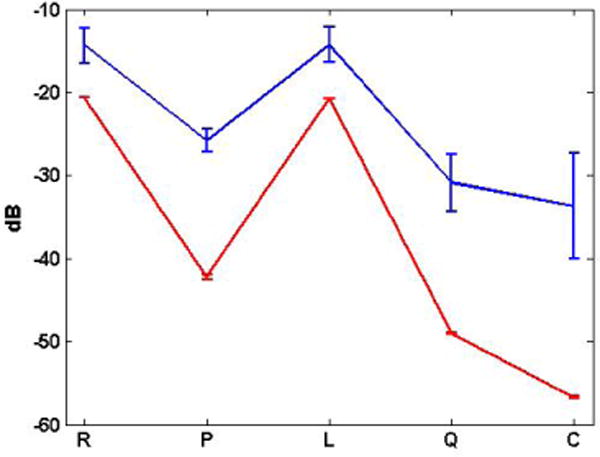
Temporal mean and standard deviation of power in a small region containing the cellulose tube for the linear RF (R), pulse inversion (P), LB-mode (L), QB-mode (Q), and CB-mode (C) images.

3) Spectral Characterization of Contrast Enhancement

Figure 8 shows the spectrograms of PI, linear, quadratic and cubic data from A-line # 52 with saline (top) and UCA (bottom) flowing in the cellulose tube. The horizontal axis was labeled as distance (in mm) using the scaling z = cτ/2, where c is the speed of sound (assumed to be uniform) and τ is the echo time. A Hamming window of length 64 was used in computing the spectrogram to preserve the axial resolution while maintaining a reasonable frequency resolution [31].

Fig. 8.

Spectrograms of the A-line through the cellulose channel while pumping saline (top) and UCA (bottom) at a rate of 6 mL/h.

The spectrograms obtained from the VF components, especially the nonlinear ones, showed an increase in signal level at ≈ 30 mm axially, which corresponded to the channel depth. The contrast between the UCA solution and saline flow cases was clear for the PI, quadratic, and cubic components. The RF data (not shown) produced similar spectrograms to the linear VF results shown in Figure 8 b) & f).

The spectra of linear VF (and RF) showed enhanced response due to the channel in the fundamental band (mainly in the 4 – 6 MHz range). Spectral broadening was observed in the presence of UCA. The PI data with UCA produced broad enhancement in the 2 – 9 MHz range, which was clearly above the signal level. We note, in realistic imaging situations with linear array probes, the PI signal has substantial residual tissue component resulting from incomplete cancellation of linear echoes at the sidelobe level.

The nonlinear VF components produced distinct enhancement at the channel location before and after infusing the UCA solution in a much wider frequency range. The spectrograms revealed that both the quadratic and cubic echo components were sensitive to the channel walls even without UCA. However, the differences between the wall and UCA enhancements were pronounced.

4) Summary of Phantom Imaging Results

The contrast-to-tissue ratios defined in Equations 6&7 provide a measure of sensitivity to the channel without and with UCA, respectively. Table I shows the CTR_saline & CTR_UCA values for the PI, LB-mode, QB-mode, and CB-mode. These values demonstrate, consistent with the graphical results in Figures 6&8, that the nonlinear VF components achieve CTR enhancement by suppressing, not eliminating tissue components.

TABLE I.

CTR Values in dB (mean ± std)

	PI	Linear	Quadratic	Cubic
CTRsaline	3.9±0.3	2.7±0.0	2.8±0.1	4.6±0.1
CTRUCA	20.2±1.4	9.2±2.1	21.0±3.4	27.8±6.3

The size of the cellulose channel (200 µm inner diameter and 280µm outer diameter) was smaller than the speckle correlation cell size [28] for the LA14-5/38 probe in the vicinity of the channel (0.62 mm lateral and 0.32 mm axial). Therefore, the extent of the channel estimated using echogenicity is a measure of the spatial specificity. Table II shows the spatial extent of the UCA region in each image component based on direct measurement from line graphs such as those shown in Figure 6. A pixel was included in the UCA region if its mean echogenicity was separated from the tissue mean echogenicity by more than one standard deviation. While the spatial extent was a coarse measurement, especially in the lateral direction, it served to illustrate the sensitivity of the different methods to sidelobe artifacts. In this case, the PI method produced the largest spatial extent, which resulted from imperfect cancellation of echo components due to the sidelobes of the imaging beams.

TABLE II.

Spatial extent of UCA Activity

	PI	Linear	Quadratic	Cubic
Axial, mm	0.9	0.5	0.5	0.5
Lateral, mm	1.2	0.6	0.6	0.6

The results shown in Tables I and II are representative of all the frames collected and allow for the following summary:

1. The quadratic component of the VF produced similar levels of sensitivity (CTR_UCA) as PI while offering a higher dynamic range and better spatial specificity.

2. The cubic component of the VF outperformed the other methods in terms of CTR values, spatial specificity and improved dynamic range.

B. VF Order, Memory and RLS Parameter Selection

VF Order

In general, the order of nonlinearity of the VF filter (i.e. quadratic, cubic, quartic, etc.) should be chosen to match the expected nonlinearity of the echo data. For the low-MI imaging scenarios of interest in the ultrasound imaging technology, the 2nd and 3rd order VFs may be sufficient and are supported by the levels of enhancement reported herein and in previous publications [16]. However, a formal approach to VF order selection is still being investigated.

The VF Memory, m

The memory of the VF filter depends on the nature of the nonlinearity. For example, a static nonlinearity such as a square-law device can be captured with zero memory, m = 1 in (1). Microbubbles oscillating according to the Rayleigh-Plesset equation [32] or similar dynamic models requires larger values of m to capture these dynamics. The default value of m = 15 represents a memory of 0.375 µs at a sampling frequency of 40 MHz. However, similar results were achieved for the range 3 ≤ m ≤ 30. For example, m = 11 and m = 19 produced very similar results in terms of UCA enhancement spectral bands. On the other hand, m = 30 resulted in deterioration in UCA enhancement bands. This can be attributed to the fact that the matrix G became increasingly more ill-conditioned as we increased m, which can result in inaccurate solution to the MNLS problem in (2).

The Convergence of the TVF

The main advantage of the RLS algorithm is its robustness and guaranteed convergence. In the context of linear filtering, the convergence is within 2m iterations for an order m filter. For the kernels shown in this paper, the number of independent coefficients was in the hundreds, but the convergence was achieved within 200 – 300 iterations (samples) with well-behaved learning curves.

Deriving the Filter Coefficients with Tissue Data Only

For the results presented so far, we derived the filter coefficients using the RF data containing echoes from the cellulose tube while pumping the UCA solution. We refer to this filter as the ‘UCA filter’. In our experience, training the filter using UCA data is not critically important. Other ‘tissue filters’ can be derived from RF data containing echoes from tissue. Figure 9 shows the temporal mean and standard deviation plots resulting from two different ‘Tissue Filters’ (red) compared to the results obtained using the ‘UCA Filter’ (black). These results show that the VF kernel coefficients depend on the training, but the behavior remains the same. It is interesting to note that the quadratic kernel exhibited larger sensitivity than the linear and cubic kernels.

Fig. 9.

Temporal mean and standard deviation of the power at the cellulose tube region using the outputs of different TVFs.

C. UCA Imaging In Vivo

Figure 10 shows grayscale images of the LNCaP tumor without (left) and with UCA (right) in B-mode (55 dB), QB-mode (120 dB), and CB=mode (185 dB). The dynamic ranges for the different image components were chosen based on the low-echogenicity region in the center of the tumor (noise floor) with reference to the specular echoes from the skin (0 dB). For B-mode, the average echogenicity of this region was ≈−50 dB and the dynamic range was set at 55 dB. For QB-mode and CB-mode, the echogenicity levels were −115 dB and −180 dB and the corresponding dynamic ranges were set to 120 dB and 185 dB, respectively.

Fig. 10.

Grayscale images of the tumor and surrounding tissues without (left) and with (right) UCA. Top: B-mode (55 dB). Middle: QB-mode (120 dB). Bottom: CB-mode (185 dB).

A subtle but appreciable difference in the echogenicity of the tumor was established after UCA injection. The changes were even more pronounced when reviewing the sequence of frames in Cine loop. For example, the lower left quadrant of the tumor showed significant increase in echogenicity after UCA injection with pronounced dynamic changes from frame to frame, indicating high UCA activity. The center of the tumor maintained its low echogenicity, but we observed sporadic localized changes consistent with microbubble flow in isolated vessels. This indicated a low-perfusion region with microflow conditions. The right side of the tumor maintained its low echogenicity throughout, indicating a low or no perfusion region. The sensitivity to UCA was also clear in the high-echogenicity tissue regions surrounding the tumor.

Figure 11 shows examples of power spectral density representations from the two regions in Figure 10 (large boxes with dashed edge lines). The box on the left contained mostly tumor tissue that exhibited heterogeneous echogenicity distribution. The box on the right was completely within normal tissues with more homogeneous echogenicity. Figure 11(a) shows the average normalized PSDs (W/Hz) for the VF filter components in the tissue region without and with UCA. The third-order VF were derived with system order m = 13, forgetting factor λ = 0.999 and regularization parameter α = −0.4. For the linear components, the differences in the PSDs without and with UCA were subtle. On the other hand, the quadratic and cubic components in the presence of UCA showed marked increase over wide range of frequencies. The situation was similar in the region containing tumor tissues with heterogeneous echogenicity as seen in Figure 11(b), but the relative enhancements in the quadratic and cubic components were lower. Figure 11(c) illustrates the quality of signal prediction achieved by the VF by plotting the PSDs of the RF data (Input) and the VF components from the tissue region in the presence of UCA. As expected, the linear component was dominant and its PSD almost matched that of the input. The quadratic and cubic components were approximately 30 and 50 dB below the linear, respectively.

Fig. 11.

Normalized power spectral density (W/Hz) for the VF components: (a) In the tissue region within the dashed box on the right (Fig. 10). (b) In the tumor region within the dashed box on the left (Fig. 10). (c) The PSDs of the VF filter components in the tissue region plotted together with the PSD of the input RF data. The linear component with UCA exhibited spectral broadening and slight increase in power compared to the linear component without UCA. These effects were more pronounced for the quadratic and cubic components. Furthermore, the enhancement levels were different in tissue and tumor regions.

Figure 12 shows the temporal mean and standard deviation of the power in regions R1, R2, R3 and R4 indicated by the solid boxes in Figure 10. The size of each region was N′ × M′ = 13 × 7. Region 1 was located in a well-perfused segment of the tumor while Region 2 was located in a poorly-perfused segment with isolated microflow. Region 3 was located in a low-perfused, high-echogenicity segment of the tissue surrounding the tumor. Region 4 was located in a low-echogenicity segment of the tumor with no apparent perfusion. The classification of perfusion in each region was based on Cine loop review before and after UCA injection. It should be noted that the locations of the boxes in the images with and without UCA were corrected for small spatial shifts of ≈1.5 mm laterally and ≈0.5 mm axially.

Fig. 12.

Temporal mean and standard derivation (error bars) of the average power in the four representative regions shown in Figure 10. Data shown without (red) and with UCA (blue).

In Region 1, all image components, including B-mode, showed an increase of the mean power level as well as increased standard deviation. This was the expected result in well-perfused regions where the presence of the UCA was observed in B-mode immediately after injection. In Region 2, the B-mode showed smaller change in the mean value and marked increase in standard deviation. In Region 3, B-mode and LB-mode showed relatively the same mean value before and after UCA injection with a slight increase in the standard deviation. The nonlinear components showed greater separation in the mean values and a slight increase in the standard deviation after injection. In Region 4, the statistics were practically the same with or without UCA indicating low or no perfusion in a low scattering region.

A comparison between the echogenicities of Regions 2 & 4 in Fig. 10 led to an interesting difference that helped to shed some light on the advantages of nonlinear filtering. Note that, in the absence of UCA, both regions had the same values of average power (both mean and standard deviation). In the presence of UCA, Region 2 exhibited significant increase in the standard deviation compared to Region 4. In reviewing the imaging frames in Cine loop with UCA, it was clear that an isolated vessel ran through R2 in the axial direction as evidenced by a localized echo moving towards the transducer. To illustrate this point, we show (Figure 13) spatio-temporal echogenicity maps (M-mode) for the vertical line segments passing through Region 2 before (top) and after (bottom) UCA injection. The conventional M-mode images shown on the left were obtained using the RF data from 144 and 160 frames collected before and after UCA injection, respectively. The dB range of [−80,−29] was set with reference to the maximum value used to set the dB range of the B-mode image in Fig. 10.

Fig. 13.

Top: Spatio-temporal representation of the echogenicity from the A-line segment indicated by the vertical line in the top left image of Fig. 10. Bottom: Spatio-temporal representation of the echogenicity from the A-line segment indicated by the vertical line in the top right image of Fig. 10. Left to right: RF, quadratic and cubic signals, respectively. Each pair of images with and without UCA was normalized to the same dB scale.

In the presence of UCA, the M-mode image revealed an upward movement of blood in a microvessel aligned with the imaging slice. For example, a “microbubble event” appears in Frame 1 at an axial distance of 17.5 mm and moves up to an axial distance of 15.5 before disappearing in Frame 75. The M-mode data shows that the low echogenicity portion within the line segment ([15,17.5] mm) was dominated by clutter and noise components. The noise was responsible to the graininess of the echogenicity values, both spatially and temporally. The clutter produced semi-regular echo components, which could result from reverberation and/or beamforming artifacts given the cyst-like nature of this portion of the tumor.

Figure 13 also shows the corresponding QM-mode ([−165,−84] dB) and CM-mode ([−238,−142] dB) representations of the echogenicity for the same A-line segments. These showed the same microbubble events, but with significant noise reduction compared to M-mode (evidenced by the absence of the graininess in both components). In addition, QM-mode and CM-mode produced higher reduction in clutter components compared to M-mode. For example, M-mode showed persistent clutter patterns at 15.8 and 16.1 mm axially with intensity levels close to those generated by the microbubble event. These clutter patterns were substantially suppressed in QM-mode and CB-mode. The suppression of the noise and other clutter in low scattering regions could be the key to imaging low-level UCA activity in heterogeneously perfused tumors.

D. Remarks on In Vivo Results

The LNCaP tumor model provided an excellent example of a region with heterogeneous perfusion. For example, the temporal dynamics of UCA activity in the lower left quadrant (where Region 1 was located) were consistent with the presence of “blood lakes”, a characteristic of this tumor. On the other hand, the dynamics in Region 2 were consistent with microflow in an isolated vessel. The performance of the TVF components in terms of improving the sensitivity and specificity to UCA activity was supported by observing the dynamics of the echoes in Cine loop and on M-mode. Though we have presented in vivo data from one animal, the results reported here are typical of numerous data sets obtained from tumor-bearing mice [19] and rat brain [33]. The significance of the LNCaP tumor data is that it provided different regions within the tumor with different perfusion and/or echogenicity characteristics, which may be more clinically relevant than small-animal tumors with uniform perfusion characteristics.

In this paper, we summarized the temporal (frame-to-frame) behavior of the power levels by computing the temporal mean and standard deviation over all available frames. To compare these values with and without UCA, we compensated for the shift in probe position between the two acquisitions. Fortunately, motion was not a factor during acquisition where we only observed ≈ 0.1 mm axial motion during gasps (as can be gleaned from the M-mode data in Fig. 13). A better approach to demonstrate the contrast enhancement, however, is to use running temporal statistics and account for motion as we have proposed earlier [30]. Briefly, a temporal perfusion index (TPI) is defined to reward the temporal changes in echogenicity while suppressing the variation due to noise and motion. The TPI approach as it applies to in vivo tumor perfusion imaging will be reported elsewhere.

V. Conclusion

Polynomial filtering provides a powerful signal processing tool to image UCA activity with high sensitivity and spatial specificity. Imaging of UCA in a 200-µm cellulose tube embedded in a tissue-mimicking phantom was performed to confirm these capabilities. B-mode and PI images were used as reference to characterize the performance of the nonlinear VF components. QB-mode images produced similar levels of sensitivity as PI while providing higher spatial specificity and dynamic range. CB-mode images produced higher levels of sensitivity and spatial specificity than PI with even larger increase in dynamic range.

Results from in vivo tumor imaging demonstrated the ability of the TVF components to produce enhanced UCA echogenicity in regions characterized by high and low perfusion. Nonlinear VF components achieved increased mean and/or standard deviation of the echogenicity in response to UCA. The increase in the standard deviation reflected the sporadic UCA activity in small vessels as confirmed by the M-mode results and the review in Cine loop. Significantly, the changes in the mean and standard deviation in vivo were consistent with the results from the cellulose channel in tissue-mimicking phantom.

Furthermore, results from in vivo experiments demonstrated that the nonlinear VF components lower the noise floor by the combined effect of noise rejection and reduction of the clutter. This offers the promise of high-specificity imaging of heterogeneous perfusion for characterization of tumors, plaques, ischemic tissues, etc.

Biographies

Juan Du received her B.Sc. degree in Control, Detection and Navigation in 2009 from the Beihang University (BUAA), Beijing, China, and M.Sc. degree in Electrical Engineering in 2012 from the University of Minnesota, Twin Cities, MN, USA. Now, she is working toward the Ph.D. degree in Electrical Engineering at the University of Minnesota, Twin Cities.

Her current research interests include: ultrasound microvascular imaging, biomedical-related signal processing, and DSP design and implementation.

Dalong Liu received the B.Sc. and M.Sc. degrees in biomedical engineering from Zhejiang University, Hangzhou, China, in 2001 and 2004, respectively. He received the Ph.D. degree in biomedical engineering from the University of Minnesota, Minneapolis, MN, USA, in 2010.

Dr. Liu used to work with Siemens Medical Solutions, Malvern, PA, USA. He is currently a research assistant professor at the University of Minnesota, Twin Cities, MN, USA. His research interests include ultrasound imaging, ultrasound elastography and thermography, ultrasound system design.

Emad S. Ebbini (S′82–M′90–SM′08–F′11) received the B.Sc. degree in EE/communications in 1985 from the University of Jordan, Amman, Jordan, and the M.S. and Ph.D. degrees in EE from the University of Illinois at Urbana-Champaign, Urbana, IL, USA, in 1987 and 1990.

From 1990 to 1998, he was with the faculty of the Department of Electrical Engineering and Computer Science, University of Michigan Ann Arbor. Since 1998, he has been with the Department of electrical and computer engineering, University of Minnesota, Minneapolis, MN, USA. His research interests include signal and array processing with applications to biomedical ultrasound and medical devices.

Dr. Ebbini was a member of AdCom for the IEEE Ultrasonics, Ferroelectrics, and Frequency Control between 1994 and 1997. In 1996, he was a Guest Editor for a special issue on therapeutic ultrasound in the IEEE TRANSACTIONS ON ULTRASONICS, FERROELECTRICS, AND FREQUENCY CONTROL. He was an Associate Editor for the same transactions from 1997 to 2002. He is a member of the standing technical program committee for the IEEE Ultrasonics Symposium. He served as a member of the Board of the International Society for Therapeutic Ultrasound (2002 – 2011) and served as its President (2012 – 2015). In 1993, he received the NSF Young Investigator Award for his work on new ultrasound phased arrays for imaging and therapy.

References

- 1.Burns PN, Wilson SR. Microbubble contrast for radiological imaging: 1. principles. Ultrasound Q. 2006 Mar;22(1):5–13. [PubMed] [Google Scholar]
- 2.Wang X, Liang H-D, Dong B, Lu Q-L, Blomley MJK. Gene transfer with microbubble ultrasound and plasmid dna into skeletal muscle of mice: comparison between commercially available microbubble contrast agents. Radiology. 2005 Oct;237(1):224–229. doi: 10.1148/radiol.2371040805. [Online]. Available: http://dx.doi.org/10.1148/radiol.2371040805. [DOI] [PubMed] [Google Scholar]
- 3.Hwang JH, Brayman AA, Reidy MA, Matula TJ, Kimmey MB, Crum LA. Vascular effects induced by combined 1-mhz ultrasound and microbubble contrast agent treatments in vivo. Ultrasound Med Biol. 2005 Apr;31(4):553–564. doi: 10.1016/j.ultrasmedbio.2004.12.014. [Online]. Available: http://dx.doi.org/10.1016/j.ultrasmedbio.2004.12.014. [DOI] [PubMed] [Google Scholar]
- 4.Eisenbrey JR, Burstein OM, Kambhampati R, Forsberg F, Liu J-B, Wheatley MA. Development and optimization of a doxorubicin loaded poly(lactic acid) contrast agent for ultrasound directed drug delivery. J Control Release. 2010 Apr;143(1):38–44. doi: 10.1016/j.jconrel.2009.12.021. [Online]. Available: http://dx.doi.org/10.1016/j.jconrel.2009.12.021. [DOI] [PMC free article] [PubMed] [Google Scholar]
- 5.Williams R, Hudson JM, Lloyd BA, Sureshkumar AR, Lueck G, Milot L, Atri M, Bjarnason GA, Burns PN. Dynamic microbubble contrast-enhanced us to measure tumor response to targeted therapy: a proposed clinical protocol with results from renal cell carcinoma patients receiving antiangiogenic therapy. Radiology. 2011 Aug;260(2):581–590. doi: 10.1148/radiol.11101893. [Online]. Available: http://dx.doi.org/10.1148/radiol.11101893. [DOI] [PubMed] [Google Scholar]
- 6.Anderson CR, Hu X, Zhang H, Tlaxca J, Declves A-E, Houghtaling R, Sharma K, Lawrence M, Ferrara KW, Rychak JJ. Ultrasound molecular imaging of tumor angiogenesis with an integrin targeted microbubble contrast agent. Invest Radiol. 2011 Apr;46(4):215–224. doi: 10.1097/RLI.0b013e3182034fed. [Online]. Available: http://dx.doi.org/10.1097/RLI.0b013e3182034fed. [DOI] [PMC free article] [PubMed] [Google Scholar]
- 7.Faez T, Emmer M, Kooiman K, Versluis M, van der Steen A, de Jong N. 20 years of ultrasound contrast agent modeling. IEEE Trans Ultrason Ferroelectr Freq Control. 2013 Jan;60(1):7–20. doi: 10.1109/TUFFC.2013.2533. [Online]. Available: http://dx.doi.org/10.1109/TUFFC.2013.2533. [DOI] [PubMed] [Google Scholar]
- 8.Goldberg BB, Liu J-B, Forsberg F. Ultrasound contrast agents: A review. Ultrasound in Medicine and Biology. 1994;20(4):319–333. doi: 10.1016/0301-5629(94)90001-9. [DOI] [PubMed] [Google Scholar]
- 9.Uhlendorf V. Physics of ultrasound contrast imaging: scattering in the linear range. Ultrasonics, Ferroelectrics, and Frequency Control, IEEE Transactions on. 1994 Jan;14(1):70–79. [Google Scholar]
- 10.Dijkmans P, Juffermans L, Musters R, van Wamel A, ten Cate F, van Gilst W, Visser C, de Jong N, Kamp O. Microbubbles and ultrasound: from diagnosis to therapy. European Heart Journal, Cardiovascular Imaging. 2004 Aug;5(4):245–256. doi: 10.1016/j.euje.2004.02.001. [DOI] [PubMed] [Google Scholar]
- 11.Haider B, Chiao R. Higher order nonlinear ultrasonic imaging. IEEE Ultrasonics Symposium Proceedings. 1999 Oct;2:1527–1531. [Google Scholar]
- 12.Brock-Fisher G, Poland M, Rafter P. Means for increasing sensitivity in nonlinear ultrasound imaging systems. The Journal of the Acoustical Society of America. 1997 Jan; [Google Scholar]
- 13.Eckersley RJ, Chin CT, Burns PN. Optimising phase and amplitude modulation schemes for imaging microbubble contrast agents at low acoustic power. Ultrasound Med Biol. 2005 Feb;31(2):213–219. doi: 10.1016/j.ultrasmedbio.2004.10.004. [Online]. Available: http://dx.doi.org/10.1016/j.ultrasmedbio.2004.10.004. [DOI] [PubMed] [Google Scholar]
- 14.Simpson DH, Chin CT, Burns PN. Pulse inversion doppler: a new method for detecting nonlinear echoes from microbubble contrast agents. IEEE Trans Ultrason Ferroelectr Freq Control. 1999;46(2):372–382. doi: 10.1109/58.753026. [Online]. Available: http://dx.doi.org/10.1109/58.753026. [DOI] [PubMed] [Google Scholar]
- 15.Tremblay-Darveau C, Williams R, Milot L, Bruce M, Burns PN. Combined perfusion and doppler imaging using plane-wave nonlinear detection and microbubble contrast agents. IEEE Trans Ultrason Ferroelectr Freq Control. 2014 Dec;61(12):1988–2000. doi: 10.1109/TUFFC.2014.006573. [Online]. Available: http://dx.doi.org/10.1109/TUFFC.2014.006573. [DOI] [PubMed] [Google Scholar]
- 16.Phukpattaranont P, Ebbini ES. Post-beamforming second-order volterra filter for pulse-echo ultrasonic imaging. IEEE Trans Ultrason Ferroelectr Freq Control. 2003 Aug;50(8):987–1001. doi: 10.1109/tuffc.2003.1226543. [DOI] [PubMed] [Google Scholar]
- 17.Al-Mistarihi M, Phukpattaranont P, Ebbini E. Post-beamforming third-order volterra filter (thovf) for pulse-echo ultrasonic imaging,” in. Acoustics, Speech, and Signal Processing, 2004 Proceedings (ICASSP ’04) IEEE International Conference on. 2004 May;3:iii-97–100. vol.3. [Google Scholar]
- 18.Al-Mistarihi M, Ebbini E. Quadratic pulse inversion ultrasonic imaging (qpi): detection of low-level harmonic activity of microbubble contrast agents [biomedical applications],” in. Acoustics, Speech, and Signal Processing, 2005 Proceedings (ICASSP ’05) IEEE International Conference on. 2005 Mar;2:ii/1009–ii/1012. Vol. 2. [Google Scholar]
- 19.Wan Y, Visaria R, Bischof J, Ebbini E. Quadratic b-mode and pulse inversion imaging of perfusion defects in vivo,” in. Life Science Systems and Applications Workshop, 2007 LISA 2007 IEEE/NIH. 2007 Nov;:237–240. [Google Scholar]
- 20.Du J, Ballard J, Choi J, Bischof J, Ebbini E. Adaptive third-order volterra filter for detection and tracking of nonlinear oscillations in ultrasound echo data,” in. Acoustics, Speech and Signal Processing (ICASSP), 2013 IEEE International Conference on. 2013 May;:1051–1055. [Google Scholar]
- 21.Du J, Liu D, Ebbini E. Contrast enhanced ultrasound imaging using adaptive third-order volterra filter,” in. Ultrasonics Symposium (IUS), 2014 IEEE International. 2014 Sep;:1746–1749. [Google Scholar]
- 22.Koh T, Powers E. Second-order volterra filtering and its application to nonlinear system identification. Acoustics, Speech and Signal Processing, IEEE Transactions on. 1985 Dec;33(6):1445–1455. [Google Scholar]
- 23.Sicuranza G. Quadratic filters for signal processing. Proceedings of the IEEE. 1992 Aug;80(8):1263–1285. [Google Scholar]
- 24.Mattera D, Paura L. Exploitation of cyclostationarity for identifying nonlinear volterra systems by input-output noisy measurements,” in. Conference Record of the Thirtieth Asilomar on Signals, Systems and Computers. 1996 Nov;1:166–170. [Google Scholar]
- 25.Meenavathi MB, Rajesh K. Volterra filtering techniques for removal of gaussian and mixed gaussian-impulse noise. International Journal of Electrical, Computer, Energetic, Electronic and Communication Engineering. 2007;1(2):176–182. [Google Scholar]
- 26.Haykin SO. Adaptive Filter Theory. 4th. Prentice Hall; Jan, 2001. [Google Scholar]
- 27.Nightingale KR, Palmeri ML, Nightingale RW, Trahey GE. On the feasibility of remote palpation using acoustic radiation force. J Acoust Soc Am. 2001 Jul;110(1):625–634. doi: 10.1121/1.1378344. [DOI] [PubMed] [Google Scholar]
- 28.Wagner RF, Insana MF, Smith SW. Fundamental correlation lengths of coherent speckle in medical ultrasonic images. IEEE Trans Ultrason Ferroelectr Freq Control. 1988;35(1):34–44. doi: 10.1109/58.4145. [Online]. Available: http://dx.doi.org/10.1109/58.4145. [DOI] [PMC free article] [PubMed] [Google Scholar]
- 29.Tuxhorn JA, McAlhany SJ, Dang TD, Ayala GE, Rowley DR. Stromal cells promote angiogenesis and growth of human prostate tumors in a differential reactive stroma (drs) xenograft model. Cancer Res. 2002 Jun;62(11):3298–3307. [PubMed] [Google Scholar]
- 30.Du J, Ballard J, Choi J, Bischof J, Ebbini E. Dynamic imaging of tumor perfusion using contrast enhanced ultrasound: In vivo results,” in. Biomedical Imaging (ISBI), 2014 IEEE 11th International Symposium on. 2014 Apr;:49–52. [Google Scholar]
- 31.Oppenheim AV, Schafer RW. In: Discrete-time Signal Processing. Oppenheim AV, editor. Prentice Hall; 2010. [Google Scholar]
- 32.Hamilton MF. In: Nonlinear Acoustics. Hamilton MF, Blackstock DT, editors. Academic Press; 1998. [Google Scholar]
- 33.Du J, Liu D, Ebbini ES. In vivo transcranial imaging of blood perfusion in rat brain using contrast-enhanced ultrasound,” in. Ultrasonics Symposium (IUS), 2015 IEEE International. 2015 Oct;:1–4. [Google Scholar]