Image reconstruction and scan configurations enabled by optimization-based algorithms in multispectral CT

Abstract

Optimization-based algorithms for image reconstruction in multi-spectral (or photon-counting) computed tomography (MCT) remains a topic of active research. The challenge of optimization-based image reconstruction in MCT stems from the inherently non-linear data model that can lead to a non-convex optimization program for which no mathematically exact solver seems to exist for achieving globally optimal solutions. In the work, based upon a non-linear data model, we design a non-convex optimization program, derive its first-order-optimality conditions, and propose an algorithm to solve the program for image reconstruction in MCT. In addition to consideration of image reconstruction for standard scan configuration, an emphasis of the work is on investigating the algorithm’s potential for enabling non-standard scan configurations with no or minimum hardware modification to existing CT systems, which can be of potential practical implications for lowered hardware cost, enhanced scanning flexibility, and reduced imaging dose/time in MCT. Numerical studies are carried out for verification of the algorithm and its implementation, and for a preliminary demonstration and characterization of the algorithm in reconstructing images and in enabling non-standard configurations with varying scanning angular range and/or X-ray illumination coverage in MCT.

1. Introduction

There is an increased level of interest and effort in research and development of multispectral (or photon-counting) computed tomography (MCT) in recent years, fueled by the advances in detector technology and system development [1–7] and by the expectation of its potential clinical benefit [8–12]. In realistic CT imaging, a non-linear data model is necessary for incorporating appropriately the product of incident X-ray spectrum and detector-energy response, which is referred to as X-ray spectrum. In MCT, multiple sets of data are collected with different X-ray spectra, and one seeks to determine basis images, which can then be used to form CT images at X-ray energies of interest.

Methods have been developed that first compensate approximately for the nonlinear effect by decomposition of data collected into X-ray transforms of individual basis images and then reconstruct basis images through the inversion of the X-ray transforms estimated [4, 13–16]. There also exist methods that were developed based upon a linear X-ray transform for approximately reconstructing images individually or jointly from the data sets and subsequently forming the basis images by linear combination of the reconstructed images [17–19]. Interest exists in developing the one-step inversion approach to reconstructing basis images directly from data collected by inverting the non-linear data model [20–26].

A carefully designed one-step inversion approach may be exploited to reconstruct basis and monochromatic images in MCT for a variety of scan configurations or systems of potential practical significance. We investigate in the work an optimization-based one-step inversion approach in which an algorithm is developed to reconstruct basis images through solving numerically a non-convex optimization program based upon the non-linear data model in MCT. In particular, we demonstrate the algorithm potential for enabling non-standard scanning configurations of practical significance involving no or minimum hardware modification.

The paper is organized as follows. In Section 2, we describe the development of the one-step inversion approach, which includes non-linear data models, a non-convex optimization program, an algorithm for numerically solving the program, and convergence conditions. Section 3 summerizes the study design, including spectra, phantoms, and configurations. Following the verification and characterization studies on the algorithm in Sections 4 and 5, we carry out in Section 6 an investigation to demonstrate the potential of the algorithm proposed for enabling non-standard scanning configurations of practical implications. Discussion of the algorithm and studies is given in Section 7.

2. Optimization-based Image Reconstruction in Multispectral CT

2.1. Continuous-to-discrete (CD)-data model

In MCT, one seeks to determine X-ray linear attenuation coefficient $f\prime (E,\overrightarrow{r})$ from knowledge of multiple transmission measurements. We decompose $f\prime (E,\overrightarrow{r})$, a function of X-ray photon energy E and spatial coordinates $\overrightarrow{r}$, into the form

$$f\prime (E,\overrightarrow{r})={\displaystyle \sum _k{\mu }_k(E)}{b}_k(\overrightarrow{r}),$$ (1)

where k ∈ ℤ⁺, and μ_k(E) and $b_k(\overrightarrow{r})$ are referred to as decomposition coefficients and basis images. The decomposition can be e.g., material or interaction based [13] depending upon how μ_k(E) is selected. Assuming that the decomposition coefficients are known, we simplify the problem of image reconstruction in MCT to the determination of the basis images, which are functions only of spatial variable $\overrightarrow{r}$. In this work, a material decomposition is considered in which the mass-attenuation coefficient of the kth basis image material is selected as μ_k(E).

Letting $Q_j^{[s]}(E)$ denote the X-ray spectrum for ray j with spectrum s, and $I_j^{[s]}$ and $I_{0j}^{[s]}$ the transmission measurements for ray j in the presence and absence, respectively, of $f\prime (E,\overrightarrow{r})$, we can define a data model as ${\stackrel{\sim }{g}}_j^{[s]}=-\ln \left(I_j^{[s]}/I_{0j}^{[s]}\right)$, which can be written further as

$${\stackrel{\sim }{g}}_j^{[s]}=-\ln {\displaystyle {\int }_0^{\infty }\mathrm{d}E}{\stackrel{\sim }{q}}_j^{[s]}(E)\exp \left(-{\displaystyle {\int }_0^{\infty }\mathrm{d}tf\prime (E,{\overrightarrow{r}}_{\mathrm{\lambda }}+t\widehat{\beta })}\right)$$ (2)

$$=-\ln {\displaystyle {\int }_0^{\infty }\mathrm{d}E}{\stackrel{\sim }{q}}_j^{[s]}(E)\exp \left(-{\displaystyle \sum _k{\mu }_k(E){\displaystyle {\int }_0^{\infty }\mathrm{d}t}{b}_k({\overrightarrow{r}}_{\mathrm{\lambda }}+t\widehat{\beta })}\right),$$ (3)

where ${\overrightarrow{r}}_{\mathrm{\lambda }}$ denotes the source position, $\widehat{\beta }$ the direction of ray j, s ∈ {1,⋯, S}, S the total number of X-ray spectra used, and

$${\stackrel{\sim }{q}}_j^{[s]}(E)=Q_j^{[s]}(E){\left({\displaystyle {\int }_0^{\infty }\mathrm{d}E}{Q}_j^{[s]}(E)\right)}^{-1}$$ (4)

the normalized spectral function satisfying $\int \mathrm{d}E{\stackrel{\sim }{q}}_j^{[s]}(E)=1$. Spectrum function ${\stackrel{\sim }{q}}_j^{[s]}(E)$ can be ray-dependent in cases that a bow-tie filter is placed in front of the X-ray source and/or that multiple measurements can be made for a given ray, e.g., using multiple energy bins in photon-counting detector.

Because ${\stackrel{\sim }{q}}_j^{[s]}(E)$, μ_k(E), and $b_k(\overrightarrow{r})$ are functions of continuous variable E or $\overrightarrow{r}$, and because ${\stackrel{\sim }{g}}_j^{[s]}$ for ray j is specified by discrete index j, we refer to equation (2) as a continuous-to-discrete (CD)-data model, which is used for obtaining discrete-to-discrete (DD)-data models below. When ${\stackrel{\sim }{q}}_j^{[s]}(E)=\delta (E-E_0)$, the CD-data model becomes the conventional X-ray transform for ray j [27].

In practical CT imaging with spectrum s, measurements made at a discrete source position $j_{\mathrm{\lambda }}^{[s]}$ form a two-dimensional (2D) array consisting of rows and columns indexed by $j_u^{[s]}$ and $j_v^{[s]}$. Let $N_{\mathrm{\lambda }}^{[s]}$ denote the total number of discrete source positions and $N_u^{[s]}$ and $N_v^{[s]}$ the total numbers of rows and columns of the detector-measurement array at the source position, we can align all the measurements into a one-dimensional (1D) array in a concatenated form in the order of $j_u^{[s]}$, $j_v^{[s]}$, and $j_{\mathrm{\lambda }}^{[s]}$, with elements indexed by $j=j_u^{[s]}+j_v^{[s]}\times N_u^{[s]}+j_{\mathrm{\lambda }}^{[s]}\times N_v^{[s]}\times N_u^{[s]},J^{[s]}=N_{\mathrm{\lambda }}^{[s]}\times N_u^{[s]}\times N_v^{[s]}$, and j ∈ {0, ⋯, J^[s]−1}.

2.2. Discrete-to-discrete (DD)-data models

The energy space can be discretized uniformly with E = mΔ_E, where m ∈ {1,⋯, M} and Δ_E the energy sampling interval. The discretized form of the normalized spectrum function in equation (4) is defined as $q_{jm}^{[s]}={\mathrm{\Delta }}_E{\stackrel{\sim }{q}}_j^{[s]}(m{\mathrm{\Delta }}_E)$ satisfying normalization condition ${\displaystyle {\sum }_m{q}_{jm}^{[s]}}=1$. We also consider a voxel-based representation of three-dimensional (3D) image space by discretizing evenly its x-, y-, and z-axis, with x = x₀ + i_xΔ_x, y = y₀ + i_yΔ_y, and z = z₀ + i_zΔ_z, where i_x ∈ {0,⋯, N_x – 1}, i_y ∈ {0,⋯, N_y – 1}, and i_z ∈ {0,⋯, N_z – 1}. N_x, N_y, and N_z denote the total numbers of voxels, Δ_x, Δ_y, Δ_z the voxel sizes and x₀, y₀, z₀ starting positions along x, y, and z-axis, respectively. The voxels can be aligned into a 1D array of size I = N_x × N_y × N_z in a concatenated form in the order of i_x, i_y, and i_z, indexed by i = i_x + i_y × N_x + i_z × N_y × N_z.

For spectrum s, using equation (2) and the discrete image array, we obtain a DD-data model as

$$g{\prime }_j^{[s]}=-\ln {\displaystyle \sum _m{q}_{jm}^{[s]}}\exp \left(-{\displaystyle \sum _i{a}_{ji}^{[s]}}{f}_{im}^{\prime }\right),$$ (5)

where j ∈ {0,⋯, J^[s] – 1}, i ∈ {0,⋯, I − 1}, $a_{ji}^{[s]}$ denotes the intersection length of ray j with voxel i, $f_{im}^{\prime }$ the discrete linear attenuation coefficient at energy m

$$f_{im}^{\prime }={\displaystyle \sum _{k\in \mathbb{Z}+}{\mu }_{km}{b}_{ki}},$$ (6)

where μ_km = μ_k(mΔ_E), and b_ki discrete basis image k at voxel i. Subscript i indicates that $f_{im}^{\prime }$ and b_ki are in the concatenated form described above.

When K basis images are considered, we obtain a discrete form of equation (1) as

$$f_{im}={\displaystyle \sum _k{\mu }_{km}{b}_{ki}}\text{and}{f}_{im}^{\prime }=f_{im}+\mathrm{\Delta }{f}_{im},$$ (7)

where k ∈ {1,⋯, K}, and Δf_im the difference between $f_{im}^{\prime }$ and f_im. We refer to f_im and Δf_im, as the monochromatic image, and the image decomposition error within voxel i at energy m. Vector images ${\mathbf{f}}_m^{\prime }$ and f_m of size I at energy m can be formed with elements f_im and $f_{im}^{\prime }$, respectively. Similarly, basis-image vector b_k of size I can be assembled in which entry i is given by b_ki.

Ignoring decomposition error Δf_im in equation (5), we obtain another DD-data model as

$$g_j^{[s]}(\mathbf{b})=-\ln {\displaystyle \sum _m{q}_{jm}^{[s]}}\exp \left(-{\displaystyle \sum _k{\mu }_{km}}{\displaystyle \sum _i{a}_{ji}^{[s]}{b}_{ki}}\right),$$ (8)

where k ∈ {1, ⋯, K}, and b denotes an aggregate basis-image vector formed by concatenating individual basis-image vectors b_k in the ascending order of k. For simplicity, we refer to b as the basis image.

The reconstruction algorithm is designed based upon the DD-data model in equation (8) in the work. When the algorithm is applied to data collected in real experiment or generated by use of a data model (e.g., equation (5)) other than equation (8), the data necessarily contain inconsistencies such as noise and/or decomposition error with the data model in equation (8).

Variable b in model data $g_j^{[s]}(\mathbf{b})$ indicates explicitly that the reconstruction task is to determine b from knowledge of data measured. Considering all of the measurements with spectrum s, we form vector g^[s](b) of size J^[s], with elements $g_j^{[s]}(\mathbf{b})$. An aggregate vector g(b) of model data can then be assembled by concatenating g^[s](b) in the ascending order of s. Additionally, ${\mathbf{q}}_j^{[s]}$ of size M is used to denote a vector of discretized spectrum in which entry $q_{jm}^{[s]}$ indicates value of spectrum s at energy m for ray j. Let $g_{\mathcal{M}j}^{[s]}$ denote the measured data for ray j with spectrum s, which can be used to form aggregate vector ${\mathbf{g}}_{\mathcal{M}}$, i.e., the counterpart of model data g(b) as discussed above.

2.3. Non-convex optimization program

Image reconstruction in MCT is tantamount to the determination of basis image b by inverting the DD-data model in equation (8) from knowledge of measured data ${\mathbf{g}}_{\mathcal{M}}$, which can be formulated as a constrained optimization program in the form of

$$\mathbf{b}\ast =\underset{\mathbf{b}}{\arg min}\mathrm{\Psi }(\mathbf{b})\mathrm{s}.\mathrm{t}.\mathrm{\Phi }(\mathbf{b};{\mathbf{g}}_{\mathcal{M}})\le \epsilon \&\mathbf{b}⪰0,$$ (9)

where data constraint parameter ε > 0, and ⪰ denotes the vector-form inequality, which requires all elements of b to be non-negative. In this work, we design the objective and data-fidelity functions as

$$\mathrm{\Psi }(\mathbf{b})={\displaystyle \sum _k{\Vert {\mathbf{b}}_k\Vert }_{\text{TV}}}\text{and}\mathrm{\Phi }(\mathbf{b};{\mathbf{g}}_{\mathcal{M}})=D(\mathbf{g}(\mathbf{b}),{\mathbf{g}}_{\mathcal{M}}),$$ (10)

where ‖·‖_TV denotes the image total-variation (TV), defined as the ℓ₁-norm of the gradient-magnitude image, i.e., ‖b_k‖_TV = ‖(|∇b_k|)‖₁, with ∇ denoting the finite-differencing approximation to the gradient and ‖·‖ a spatial magnitude operator, and D(x, y) the data divergence, often in the form of ℓ_p-norm or Kullback-Leibler (KL) divergence, between vectors x and y. We consider in this work a normalized ℓ₂-norm of vector difference between model data g(b) and measured data ${\mathbf{g}}_{\mathcal{M}}$, i.e.,

$$D(\mathbf{g}(\mathbf{b}),{\mathbf{g}}_{\mathcal{M}})={\left[\frac{{{\displaystyle {\sum }_s\Vert {\mathbf{g}}^{[s]}(\mathbf{b})-{\mathbf{g}}_{\mathcal{M}}^{[s]}\Vert }}_2^2}{{\displaystyle {\sum }_s{\Vert {\mathbf{g}}_{\mathcal{M}}^{[s]}\Vert }_2^2}}\right]}^{1/2}.$$ (11)

2.4. An algorithm for numerically solving the non-convex program

Data divergence $D(\mathbf{g}(\mathbf{b}),{\mathbf{g}}_{\mathcal{M}})$ is non-convex (NC) due to the non-linearity of the DD-data model, so is the optimization program in equations (9)-(11). In the absence of a mathematically exact solver for achieving the globally optimal solution of the non-convex optimization program, we propose instead an heuristic algorithm for numerically solving the program and demonstrate its potential in enabling MCT configurations of potential application significance.

2.4.1. Linear and non-linear contributions to the DD-data model

We first split mass-attenuation coefficient μ_km in equation (8) into [14,28]

$${\mu }_{km}={\overline{\mu }}_{jk}^{[s]}+\mathrm{\Delta }{\mu }_{\mathit{jkm}}^{[s]},$$ (12)

where

$${\overline{\mu }}_{jk}^{[s]}={\displaystyle \sum _m{q}_{jm}^{[s]}{\mu }_{km}},\text{and}\mathrm{\Delta }{\mu }_{\mathit{jkm}}^{[s]}={\mu }_{km}-{\overline{\mu }}_{jk}^{[s]}.$$ (13)

While ${\overline{\mu }}_{jk}^{[s]}$ is independent of energy as it is a spectrum-weighted average of μ_km over energy, $\mathrm{\Delta }{\overline{\mu }}_{\mathit{jkm}}^{[s]}$ remains energy dependent. Substitution of equation (12) into equation (8) yields

$$g_j^{[s]}(\mathbf{b})={\overline{g}}_j^{[s]}(\mathbf{b})+{\mathrm{\Delta }}_j^{[s]}(\mathbf{b}),$$ (14)

where j ∈ {0,⋯, J^[s] − 1},

$${\overline{g}}_j^{[s]}(\mathbf{b})={\displaystyle \sum _k{\overline{\mu }}_{jk}^{[s]}{\displaystyle \sum _i{a}_{ji}^{[s]}}{b}_{ki},}$$ (15)

and

$$\mathrm{\Delta }{g}_j^{[s]}(\mathbf{b})=-\ln {\displaystyle \sum _m{q}_{jm}^{[s]}\exp }\left(-{\displaystyle \sum _k\mathrm{\Delta }{\mu }_{\mathit{jkm}}^{[s]}}{\displaystyle \sum _i{a}_{ji}^{[s]}{b}_{ki}}\right),$$ (16)

denote linear (LI) and non-linear (NL) functions of b, respectively, and can be used to form two aggregate vectors ḡ(b) and Δg(b) in the same way of forming g(b). In particular, $\overline{\mathbf{g}}(\mathbf{b})=\mathcal{H}\mathbf{b}$ and matrix $\mathcal{H}$ is given by

$$\mathcal{H}=\left(\begin{array}{ccc}{\mathcal{U}}_1^{[1]}{\mathcal{A}}^{[1]}& {\mathcal{U}}_2^{[1]}{\mathcal{A}}^{[1]}& \dots \\ {\mathcal{U}}_1^{[2]}{\mathcal{A}}^{[2]}& {\mathcal{U}}_2^{[2]}{\mathcal{A}}^{[2]}& \dots \\ ⋮& ⋮& \ddots \end{array}\right),$$ (17)

where matrix ${\mathcal{A}}^{\left[s\right]}$, of size J^[s] × I and with element $a_{ji}^{[s]}$, denotes the discrete X-ray transform for all measurements made with spectrum s, and ${\mathcal{U}}_k^{[s]}$ a diagonal matrix of size J^[s] with diagonal elements ${\overline{\mu }}_{jk}^{[s]}$.

The DD-data model in equation (8) for an individual ray can then be re-expressed in a matrix form for all of the rays considered as

$$\mathbf{g}(\mathbf{b})-\mathrm{\Delta }\mathbf{g}(\mathbf{b})=\mathcal{H}\mathbf{b}.$$ (18)

While equation (18) is only a different form of the DD-data model in equation (8), it reveals that it is NL term Δg(b) that results in the non-convexity of the data divergence and thus of the optimization program.

2.4.2. A procedure for numerically lowering the non-convex data divergence

In an attempt to facilitate the derivation of the procedure, we first assume that NL term Δg(b) is known and denoted by $\stackrel{\sim }{\mathrm{\Delta }\mathbf{g}}$. Under this condition, the DD-data model in equation (18) becomes a linear equation, i.e., $\mathbf{g}(\mathbf{b})-\stackrel{\sim }{\mathrm{\Delta }\mathbf{g}}=\mathcal{H}\mathbf{b}$, and data divergence $D(\mathcal{H}\mathbf{b},{\mathbf{g}}_{\mathcal{M}}-\stackrel{\sim }{\mathrm{\Delta }\mathbf{g}})$ and the optimization program consequently becomes convex, which can then be solved by use of a host of well-established algorithms [29–31].

The projection-onto-convex-sets (POCS) procedure can be used to lower convex $D(\mathcal{H}\mathbf{b},{\mathbf{g}}_{\mathcal{M}}-\stackrel{\sim }{\mathrm{\Delta }\mathbf{g}})$ with the updating step

$${\mathbf{b}}_k^{(n+1)}={\mathbf{b}}_k^{(n)}+{\gamma }^{(n)}{\overline{\mu }}_{jk}^{[s]}\frac{\left[g_{\mathcal{M}j}^{[s]}-{\stackrel{\sim }{\mathrm{\Delta }g}}_j^{[s]}\right]-{\mathbf{a}}_j^{[s]}{\displaystyle {\sum }_k{\overline{\mu }}_{jk}^{[s]}{\mathbf{b}}_k^{(n)}}}{{\displaystyle {\sum }_k{({\overline{\mu }}_{jk}^{[s]})}^2{\mathbf{a}}_j^{[s]}}{\mathbf{a}}_j^{[s]\top }}{\mathbf{a}}_j^{[s]\top },$$ (19)

where j ∈ {0,⋯, J^[s] – 1}, ${\stackrel{\sim }{\mathrm{\Delta }g}}_j^{[s]}$ is the jth element with spectrum s of $\stackrel{\sim }{{\mathrm{\Delta }}_{\mathbf{g}}}$, ${\mathbf{a}}_j^{[s]}$ a row vector that is the jth row of matrix ${\mathcal{A}}^{\left[s\right]}$, ${\mathbf{a}}_j^{[s]\top }$ a column vector as the transpose of ${\mathbf{a}}_j^{[s]}$, and 0 < γ⁽ⁿ⁾ < 2.

Using b⁽ⁿ⁾ in equation (16), one can calculate

$$\mathrm{\Delta }{g}_j^{[s]}({\mathbf{b}}^{(n)})=-\ln {\displaystyle \sum _m{q}_{jm}^{[s]}}\exp \left(-{\displaystyle \sum _k\mathrm{\Delta }{\mu }_{\mathit{jkm}}^{[s]}{\mathbf{a}}_j^{[s]}}{\mathbf{b}}_k^{(n)}\right).$$ (20)

We then propose to use $\mathrm{\Delta }{g}_j^{[s]}({\mathbf{b}}^{(n)})$ as an estimate of ${\stackrel{\sim }{\mathrm{\Delta }g}}_j^{[s]}$ in equation (19), and thus obtain an NC-POCS update procedure as

$${\mathbf{b}}_k^{(n+1)}={\mathbf{b}}_k^{(n)}+{\gamma }^{(n)}{\overline{\mu }}_{jk}^{[s]}\frac{\left[g_{\mathcal{M}j}^{[s]}-\mathrm{\Delta }{g}_j^{[s]}({\mathbf{b}}_k^{(n)})\right]-{\mathbf{a}}_j^{[s]}{\displaystyle {\sum }_k{\overline{\mu }}_{jk}^{[s]}{\mathbf{b}}_k^{(n)}}}{{\displaystyle {\sum }_k{({\overline{\mu }}_{jk}^{[s]})}^2{\mathbf{a}}_j^{[s]}{\mathbf{a}}_j^{(s)\top }}}{\mathbf{a}}_j^{[s]\top },$$ (21)

which has a form identical to that of the conventional POCS, except for that at iteration n, $\mathrm{\Delta }{g}_j^{[s]}({\mathbf{b}}^{(n)})$ is calculated to compensate for the NL effect [28].

2.4.3. The ASD-NC-POCS algorithm for the non-convex program

Combining this NC-POCS procedure for lowering $D(\mathbf{g},(\mathbf{b}),{\mathbf{g}}_{\mathcal{M}})$ with the steepest descent (SD) for lowering the TV objective function, we obtain an heuristic ASD-NC-POCS algorithm for numerically solving the non-convex program specified by equations (9)-(11). Like the conventional ASD-POCS algorithm [29], the ASD-NC-POCS algorithm adaptively lowers the image TV and data divergence by use of the SD and NC-POCS procedures for image reconstruction in MCT, with its pseudo-code in Algorithm 1. In a reconstruction, once the practical convergence condition on the data constraint is satisfied, we apply gradient descent steps to further lowering data divergence so that other practical convergence conditions can be met rapidly [32]. While there is no proof whether the ASD-NC-POCS algorithm can mathematically solve the non-convex program considered, we devise below its necessary, convergence conditions.

2.5. Reconstruction parameters

There are two types of parameters involved in an optimization-based image reconstruction, which are referred to as program and algorithm parameters. The former specify the optimization program in equation (9), including image voxel, spectra ${\mathbf{q}}_j^{[s]}$, system matrices ${\mathcal{A}}^{[s]}$, and parameter ε. Different choices of program parameters necessarily lead to different optimization programs and thus different designed solutions. In this work, we focus on the investigation of ε that impacts dominantly the reconstruction, while selecting image voxel, ${\mathbf{q}}_i^{[s]}$, and ${\mathcal{A}}^{[s]}$ similar to those used in practical applications. The algorithm parameters such as γ⁽ⁿ⁾, N_TV, and α_k(n) in Algorithm 1 control the algorithm path leading to the designed solution. While they have no effect on the designed solutions, they can impact the numerical reconstructions especially for a non-convex program. In this study, we use the same algorithm parameters as those used in the conventional ASD-POCS algorithm [29].

We consider three necessary, mathematical convergence conditions for the ASD-NC-POCS algorithm:

$$\overline{D}({\mathbf{b}}^{(n)})=|D(\mathbf{g}({\mathbf{b}}^{(n)},{\mathbf{g}}_{\mathcal{M}})-\epsilon |/\epsilon \to 0$$

$$\overline{\mathrm{\Delta }}\mathrm{\Psi }({\mathbf{b}}^{(n)})=\frac{|\mathrm{\Psi }({\mathbf{b}}^{(n+1)})-\mathrm{\Psi }({\mathbf{b}}^{(n)})|}{|\mathrm{\Psi }({\mathbf{b}}^{(n+1)})+\mathrm{\Psi }({\mathbf{b}}^{(n)})|}\to 0$$ (22)

$$c_{\alpha }({\mathbf{b}}^{(n)})={\widehat{\mathbf{d}}}_{\text{data}}^{\top }({\mathbf{b}}^{(n)}){\widehat{\mathbf{d}}}_{\text{TV}}({\mathbf{b}}^{(n)})\to -1,$$

as iteration number n → ∞, where unit vectors ${\widehat{\mathbf{d}}}_{\text{data}}({\mathbf{b}}^{(n)})$ and ${\widehat{\mathbf{d}}}_{\text{TV}}({\mathbf{b}}^{(n)})$ are defined in Appendix A [29]. The second condition is for the optimality of the objective function, whereas the other two are the local optimality conditions, i.e., the Karush-Kuhn-Tucker (KKT) conditions, as shown in Appendix A. While the mathematical convergence conditions cannot be met in practical reconstructions, they are used to devise practical convergence conditions for studies discussed below.

Algorithm 1.

pseudo code for the ASD-NC-POCS algorithm

1:	Initialize ${\mathbf{b}}_k^{(0)}\leftarrow 0$, ${\widehat{\mathbf{g}}}^{(0)}\leftarrow {\mathbf{g}}_{\mathcal{M}}$
2:	repeat iterations
3:	- POCS update -
4:	for s = 1 to S do
5:	for j = 0 to J[s] − 1 do
6:	for k = 1 to K do
7:	${\mathbf{b}}_k^{(n+1)}={\mathbf{b}}_k^{(n)}+{\gamma }^{(n)}{\overline{\mu }}_{jk}^{[s]}\frac{{\widehat{g}}_j^{[s](n)}-{\mathbf{a}}_j^{[s]}{\displaystyle {\sum }_k{\overline{\mu }}_{jk}^{[s]}{\mathbf{b}}_k^{(n)}}}{{\displaystyle {\sum }_k{({\overline{\mu }}_{jk}^{[s]})}^2{\mathbf{a}}_j^{[s]}{\mathbf{a}}_j^{[s]\top }}}{\mathbf{a}}_j^{[s]\top }$
8:	end for
9:	end for
10:	end for
11:	- TV descent update -
12:	for t = 1 to NTV do
13:	for k = 1 to K do
14:	${\mathbf{b}}_k^{(n+1)}\leftarrow {\mathbf{b}}_k^{(n+1)}-{\alpha }_k^{(n+1)}{\nabla }_{{\mathbf{b}}_k}{\Vert {\mathbf{b}}_k^{(n+1)}\Vert }_{\text{TV}}$
15:	end for
16:	end for
17:	- NL term update step -
18:	for s = 1 to S do
19:	for j = 0 to J[s] − 1 do
20:	$\mathrm{\Delta }{g}_j^{[s](n+1)}=-\ln {\displaystyle \sum _m{q}_{jm}^{[s]}\exp }\left(-{\displaystyle \sum _k\mathrm{\Delta }{\mu }_{\mathit{jkm}}^{[s]}{\mathbf{a}}_j^{[s]}{\mathbf{b}}_k^{(n+1)}}\right)$
21:	${\widehat{g}}_j^{[s](n+1)}\leftarrow g_{\mathcal{M}j}^{[s]}-\mathrm{\Delta }{g}_j^{[s](n+1)}$
22:	end for
23:	end for
24:	until practical convergence conditions are satisfied

3. Numerical experiment design

3.1. Scan configuration dimensions

While the ASD-NC-POCS algorithm developed can reconstruct images from cone-beam data collected over general source trajectories, we demonstrate in the work its application to image reconstruction from data collected with a fan-beam configuration over a circular trajectory, with physical dimensions similar to those used in a standard cone-beam CT (CBCT) employed in radiation therapy. The CBCT system has source-to-detector and source-to-center-of-rotation distances of 1500 mm and 1000 mm, respectively, and a linear detector of 400 mm in length, which form a field-of-view (FOV) of 265 mm in diameter. Throughout the work, the imaged subjects are assumed to be completely within the FOV. We refer to the configuration shown in Figure 1 as a standard, full-scan configuration in which each data set is collected for spectrum s at views uniformly distributed over 2π, and use it for verification and benchmark of the algorithm implementation and performance. In addition, four non-standard configurations of practical significance are utilized for demonstrating the enabling potential of the algorithm proposed.

Figure 1.

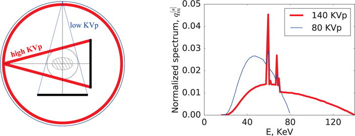
Left: Full-scan configuration in which low (thin line) and high (thick line) KVp scans are performed over 2π; and right: normalized low (thin line) and high (thick line) KVp spectra used in the studies below.

3.2. Spectra, basis images, and monochromatic images

Spectra

While the ASD-NC-POCS algorithm can be applicable to MCT with multiple (S ≥ 2) spectral measurements, we perform studies in the work using only two (i.e., S=2) spectral data sets collected with two, i.e., the low (s = 1) and high (s = 2) spectra at 80 and 140 KVp. The incident spectra are generated using the TASMICS worksheet (v1.0) [33], assuming a tungsten anode and 5-mm-Al filter, to simulate spectrum from a X-ray CT tube. The detector-energy response is modeled to be a linear energy-integrating response. The discrete X-ray spectrum, taken as the product of the incident spectrum and detector-energy response with Δ_E = 1 (KeV), is normalized and shown in Figure 1.

Basis images

We consider two (i.e., K = 2) basis images, referred to as the water and bone images, in the reconstruction. It is further assumed that the spectra are the same for all rays within one KVp scan, i.e., the discretized spectrum can be denoted by $q_m^{[s]}$, without the dependence on ray j.

Monochromatic images

Using basis images b_k reconstructed, along with knowledge of mass-attenuation coefficients, we can readily obtain monochromatic image f_m by using equation (7). In general, due to the presence of decomposition error, monochromatic image f_m represents only approximately linear attenuation coefficient image ${\mathbf{f}}_m^{\prime }$.

3.3. Phantoms

Two digital phantoms are used in the work, as shown in Figure 2. The first simulates the standardized dual-energy contrast phantom with iodine and calcium solution inserts [34], referred to as the DE-472 phantom, and the second mimics human thoracic anatomy [26], referred to as the lung phantom. Both phantoms are represented on a 512×512 array of square pixels of 0.49 mm. Each image-pixel is labeled with a material type and its density. Table 1 summarizes the materials used in the composition of the phantoms, other than water with 1.0 g/ml density. For the lung phantom simulating various human tissues, the ICRU-44 standard was used for its materials, and the mass-attenuation coefficients are readily available as tabulated data on the NIST website [35]. For the DE-472 phantom, the mass-attenuation coefficients of the iodine and calcium solutions are calculated using the XCOM web program [36], also available on the NIST website, according to the specifications of the physical GAMMEX 472 Dual Energy CT phantom [34]. As shown in Figure 2, 18 regions of interest (ROIs) in the DE-472 phantom, defined based on the inserts, and 3 ROIs of the lung phantom, defined based on material masks, are shown for computing metrics for parameter determination in the studies below.

Figure 2.

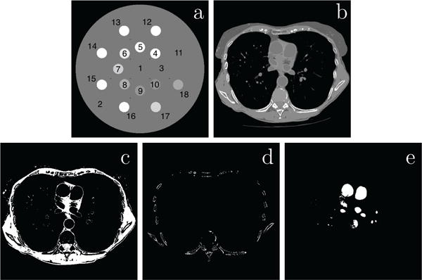
40-KeV monochromatic images of the DE-472 (a) and lung (b) phantoms. Display window: [−1000, 1000] HU. 18 ROIs within the 16 circular inserts and 2 background areas highlighted by 1 to 18 in the DE-472 phantom in (a) and 3 ROI images (row 2) for the lung phantom, indicating muscle (c), bone (d), and water (e) material masks selected for parameter selection in Secs. 5 and 6.

Table 1.

Non-water materials used in the composition of both phantoms employed in the studies.

phantom	DE-472		Lung
material	iodine solution*	calcium solution*	lung tissue	adipose tissue	skeleton muscle	cortical bone
density (g/ml)	0.002–0.02	0.05–0.6	0.1–0.6	0.88–0.95	1.11–1.21	1.53–2.05

^*indicates materials whose mass-attenuation coefficients are not readily available as tabulated data on NIST website and are thus computed using the XCOM program.

Figure 18.

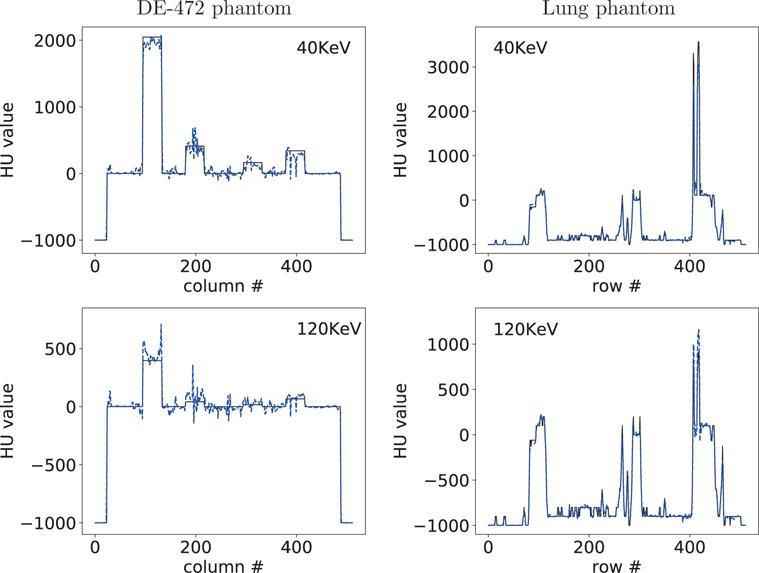
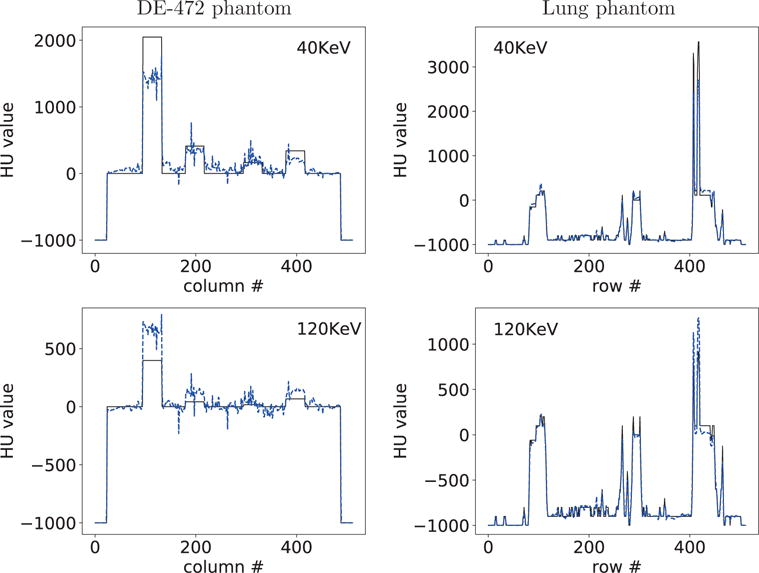
Profiles of reconstructed (dashed) and truth (solid) monochromatic energy images at 40 and 120 KeV along the horizontal and vertical lines indicated in row 2 of Figure 6 from block-illumination-scan data of the DE-472 and lung phantoms, respectively.

4. Verification study

We first perform a study to verify that under imaging conditions of interest, the ASD-NC-POCS algorithm can numerically solve the non-convex optimization program in equation (9) from ideal data generated by use of the DD-data model in equation (8) without decomposition error and noise.

4.1. Study parameters

In the study, two truth basis images representing water and cortical bone were used in equation (8) to generate ideal data from the lung phantom by use of the full-scan configuration with the low and high KVp spectra described in Figure 1. For computation efficiency, we consider an image array of I = 128 × 128 1.95-mm square pixels, and a linear detector of 256 1.56-mm bins, and generate projections at 160 views evenly distributed over 2π for each of the low and high KVp spectra. As such, the X-ray transform matrices ${\mathcal{A}}^{[1]}={\mathcal{A}}^{[2]}$ are of size J^[1] = J^[2] = 256 × 160 and I = 128 × 128. With parameters pixel, spectra, and ${\mathcal{A}}^{[s]}$ determined above, we also select parameter ε = 10⁻⁸ to form a tight solution set, as the study uses ideal data.

Based upon the mathematical convergence conditions in equation (22), we design practical convergence conditions for the verification study as

$$\overline{D}({\mathbf{b}}^{(n)})<{10}^{-4},\overline{\mathrm{\Delta }}\mathrm{\Psi }({\mathbf{b}}^{(n)})<{10}^{-4},c_{\alpha }({\mathbf{b}}^{(n)})<-\mathrm{0.99.}$$ (23)

We referred to a convergent reconstruction as one obtained when all of the convergence conditions above are satisfied. Because the truth basis images are known, we also devise a reconstruction-error metric ${\overline{\mathrm{\Delta }}}_{\mathbf{b}}({\mathbf{b}}^{(n)})=\Vert {\mathbf{b}}^{(n)}-{\mathbf{b}}_{\text{true}}{\Vert }_2/\Vert {\mathbf{b}}_{\text{true}}{\Vert }_2$, i.e., the normalized ℓ₂-distance between the truth and reconstructed basis images. This metric provides a quantitative indication as to whether and how the reconstructed basis images approach their truth counterparts.

4.2. Study results

We apply the ASD-NC-POCS algorithm to reconstructing basis images from the ideal data and display convergence results in Figure 3 and convergent reconstructions in Figure 4. It can be observed that the practical convergence conditions in equation (23) are satisfied and that convergent reconstructions are visually identical to their truth counterparts. In particular, the reconstruction-error metric in Figure 3 reveals quantitatively a small difference of the convergent reconstructions than their truth basis images, thus providing a numerical verification of the ASD-NC-POCS algorithm and its computer implementation.

Figure 3.

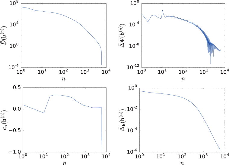
Convergence metrics $\overline{D}({\mathbf{b}}^{(n)})$, $\overline{\mathrm{\Delta }}\mathrm{\Psi }({\mathbf{b}}^{(n)})$, and c_α(b⁽ⁿ⁾), and reconstruction-error ${\overline{\mathrm{\Delta }}}_{\mathbf{b}}({\mathbf{b}}^{(n)})$ as functions of iterations n.

Figure 4.

Truth and reconstructed water- and bone-basis images. Display windows [0, 1.5]

5. Characterization study

Following the verification study with ideal data above, we perform a characterization study on the ASD-NC-POCS algorithm by using data that contain decomposition error and statistical noise, which are inconsistent with the DD-data model in equation (8).

5.1. Study parameters

For each phantom in Sec. 3.3, using its truth monochromatic image ${\mathbf{f}}_m^{\prime }$ and spectra in Fig. 1, we employ equation (5) to generate low- and high-KVp data at 640 overlapping views evenly distributed over 2π, which thus contain decomposition error. Furthermore, Poisson noise is added to data by scaling the spectra to yield 2 × 10⁴ photons per ray in the air scan. The image array of the same dimension and pixel size as the digital phantom is used in the reconstruction. At each view, projection samples are collected with a 400-mm linear detector consisting of 1024 bins of 0.39-mm size. Therefore, the X-ray transform matrices ${\mathcal{A}}^{[1]}$ and ${\mathcal{A}}^{[2]}$ are identical and of dimensions J^[1] = J^[2] = 640 × 1024 and I = 512 × 512. With the determination of program parameters, i.e., image pixel, spectra, and matrices ${\mathcal{A}}^{[s]}$, we now discuss the strategy for the selection of parameter ε in the characterization study.

Strategy for selection of parameter ε

Because data are generated directly from linear attenuation coefficient ${\mathbf{f}}_m^{\prime }$, we have no truth basis images in the characterization study. Instead, we design metrics based upon monochromatic images f_m for determination of parameter ε. R regions of interest (ROIs) in a monochromatic image are chosen for calculating the “biases” and “standard deviations” within the ROIs as

$${\theta }_{rm}={\displaystyle \sum _i|f_{im}}-f_{im}^{\prime }|/I_r\text{and}{\sigma }_{rm}={\left({\displaystyle \sum _i|f_{im}-{\theta }_{rm}{|}^2/(I_r-1)}\right)}^{\frac{1}{2}},$$

where i ∈ I_r, and I_r indicates the number of pixels within ROI r. Using θ_rm and ${\sigma }_{rm}^2$ computed at energies m₁ and m₂, we form two metrics for determination of parameter ε:

$$\Theta ={{\displaystyle \sum _r[{\theta }_{r{m}_1}^2+{\theta }_{r{m}_2}^2]}}^{\frac{1}{2}}/R\text{and}\sum ={{\displaystyle \sum _r[{\sigma }_{r{m}_1}^2+{\sigma }_{r{m}_2}^2]}}^{\frac{1}{2}}/R.$$

For a given configuration and phantom, we form monochromatic images f_m at m₁ = 80 KeV and m₂ = 140 KeV from basis images reconstructed for a number of ε values, compute Θ and Σ from the images, and then select ε that yields lowest Θ and Σ.

Practical convergence conditions

We design practical convergence conditions for the characterization study as

$$\overline{D}(b^{(n)})<{10}^{-3},\overline{\mathrm{\Delta }}\mathrm{\Psi }({\mathbf{b}}^{(n)})<{10}^{-3},c_{\alpha }({\mathbf{b}}^{(n)})<-0.5,$$ (24)

which are looser than those in the verification study as the decomposition error and data noise are considered. Our previous experience with the conventional ASD-POCS algorithm [32, 37] indicates that the third condition can often be relaxed to −0.5, instead of −0.99, with only imperceptible changes to the images. Using reconstructed basis image ${\mathbf{b}}_k^{(n)}$ in equation (7), we can readily obtain monochromatic image ${\mathbf{f}}_m^{(n)}$ at iteration n. Also, in the simulation study, we have knowledge of truth monochromatic image ${\mathbf{f}}_m^{\prime }$ and can thus calculate reconstruction-error metric ${\overline{\mathrm{\Delta }}}_{\mathbf{f}}({\mathbf{f}}_m^{(n)})=\Vert {\mathbf{f}}_m^{(n)}-{\mathbf{f}}_m^{\prime }{\Vert }_2/\Vert {\mathbf{f}}_m^{\prime }{\Vert }_2$, which is the normalized ℓ₂-distance between the truth and reconstructed monochromatic images at energy m.

5.2. Study results

Demonstration of reconstruction convergence

We first use a reconstruction from data of the full-scan configuration to demonstrate that the practical convergence conditions in equation (24) can be met by the ASD-NC-POCS algorithm. Without loss of generality, the reconstruction is carried out with ε = 0.0170, and we display in Figure 5 convergence metrics $\overline{D}({\mathbf{b}}^{(n)})$, $\overline{\mathrm{\Delta }}\mathrm{\Psi }({\mathbf{b}}^{(n)})$ and c_α(b⁽ⁿ⁾) as functions of iteration number n. It can be observed that the ASD-NC-POCS algorithm converges to meet the practical convergence conditions.

Figure 5.

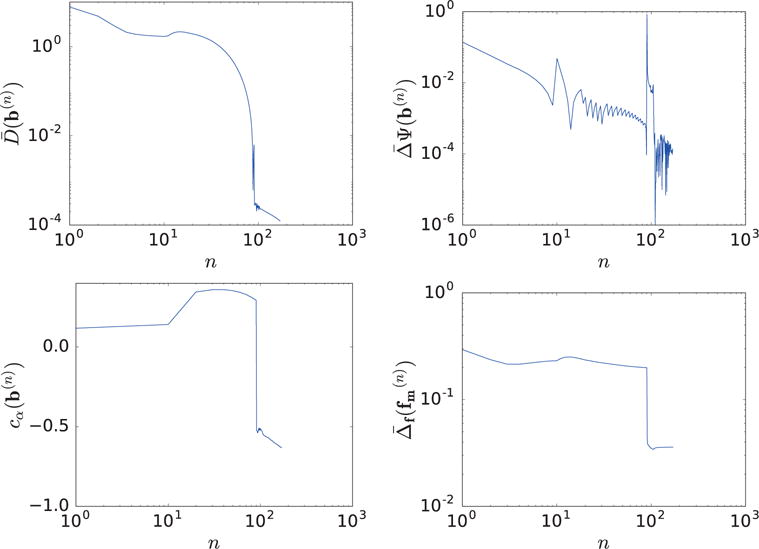
Convergence metrics $\overline{D}({\mathbf{b}}^{(n)})$, $\overline{\mathrm{\Delta }}\mathrm{\Psi }({\mathbf{b}}^{(n)})$, and c_α(b⁽ⁿ⁾), and reconstruction-error ${\overline{\mathrm{\Delta }}}_{\mathbf{f}}({\mathbf{f}}_m^{(n)})$ of 80-KeV monochromatic image obtained with ε = 0.0170, as functions of iteration number n.

Selection of parameter ε

For each of DE-472 and lung phantoms, we perform reconstructions from its data by using the ASD-NC-POCS algorithm for multiple values of ε, calculate metrics Θ and Σ from the ROIs described in section 3.3 in monochromatic energy reconstructions at 80 and 120 KeV, and select the value of ε that yields the lowest Θ and Σ. Using the strategy, we have determined ε = 0.0170 and ε = 0.0111 in the characterization study using the DE-472 and lung phantoms, respectively.

Reconstruction results

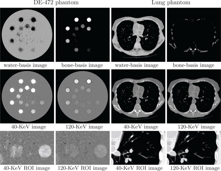
Using the program parameters (i.e., image pixel, spectra, matrices ${\mathcal{A}}^{[s]}$, and ε) determined, we reconstructed basis and monochromatic images of the DE-472 and lung phantoms. In Figure 6, we display reconstructed basis images, monochromatic images at 40 and 120 KeV used often for contrast enhancement and artifact reduction, and their zoomed-in views of ROI images enclosed by the rectangular boxes indicated in row 2.

Figure 6.

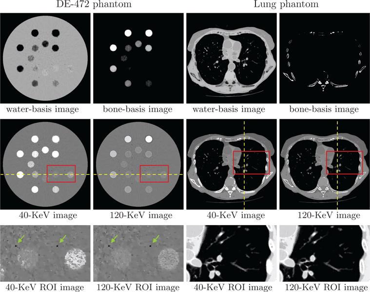
Water- and bone-basis images (row 1), 40- and 120-KeV monochromatic images (row 2), and zoomed-in views of ROI images (row 3) enclosed by boxes in row 2 from full-scan data of the DE-472 and lung phantoms, respectively, with display windows [0, 1.5] (row 1), [−1000, 1000] HU (row 2), and [−500, 500] HU (row 3, DE-472 phantom) and [−1000, 200] HU (row 3, lung phantom). The dashed lines indicate the location of the profile plots in Fig. 7, while the arrows point to the air bubbles in the DE-472 phantom.

The water-basis image retains mostly the water and soft-tissue background, while high contrast inserts and bony structures appear largely in the bone-basis image. The seemingly observable “artifacts” in basis images reconstructed are understandable because data contain decomposition error as they were generated from ${\mathbf{f}}_m^{\prime }$ instead of two basis images. However, no significant cupping or band artifacts are visible in the monochromatic images, especially for the DE-472 phantom that contains high concentration iodine and calcium inserts. ROIs of the DE-472 phantom with a narrow display window show air-bubble contrast (indicated by the arrows) and discernible contrast inserts with the lowest concentration of iodine and calcium in the phantom. Meanwhile, ROIs of the lung phantom show details of the lung nodules in the dark background, with a display window to highlight these features.

For acquiring a quantitative impression of the reconstructions, we also plot in Figure 7 profiles of truth and reconstructed monochromatic images along the horizontal and vertical lines indicated in row 2 of Figure 6. Overall, reasonably quantitative agreement in monochromatic images is observed for the lung phantom, while some discrepancy can be observed between the DE-472 phantom and its monochromatic images due to the decomposition error, and the profiles reveal that the 40-KeV monochromatic images are of contrast higher than that of the 120-KeV counterparts.

Figure 7.

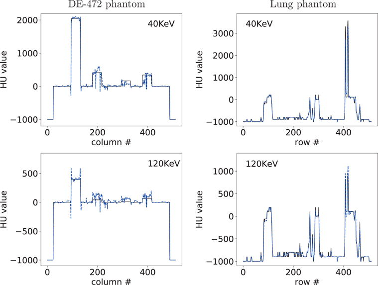
Profiles of reconstructed (dashed) and truth (solid) monochromatic images at 40 and 120 KeV along the horizontal and vertical lines indicated in row 2 of Figure 6 from full-scan data of the DE-472 and lung phantoms, respectively.

It is of practical interest in inspecting how the reconstruction of monochromatic image evolves as iterations increase. Without loss of generality, we show in Figure 8 reconstructions of 120-KeV monochromatic image at intermediate iterations for both phantoms. It appears that reconstructions at as early as iteration 50 can visually resemble the respective convergent reconstructions. Similar observations can also be made for monochromatic energy images reconstructed at other energies.

Figure 8.

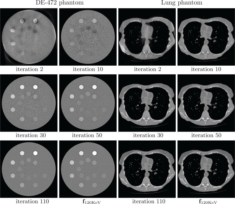
120-KeV monochromatic images of the DE-472 and lung phantoms from full-scan data at iterations 2, 10, 30, 50, and 110, along with the convergent reconstructions f_120KeV. Display window: [−1000, 1000] HU.

6. Enabling non-standard configurations

In the studies below, we investigate image reconstruction for non-standard configurations of potential application significance enabled by the ASD-NC-POCS algorithm. For each of the non-standard configurations considered, we have performed a verification study, which is not shown because results and conclusion similar to those in Sec. 4 can be obtained. Instead, we focus on characterization studies similar to that in Sec. 5 in which data contain decomposition error and statistical noise. For each of the configurations and spectra in Figure 1, we generated data from each of the DE-472 and lung phantoms by using equation (5), and added Poisson noise to the data by considering a total count level identical to that in the full-scan study in Sec. 5. Furthermore, image pixel size and spectra used are also identical to those in the study in Sec. 5, while matrices ${\mathcal{A}}^{[s]}$ are illustrated in, and parameter ε is determined by use of the strategy described in Sec. 5.1 for, each of the non-standard configurations.

6.1. Configurations with varying angular coverages

The first two non-standard configurations, as shown in Figure 9, involve varying angular coverages, and are referred to as the sparse-view and limited-angular-range configurations, respectively. In the former, low- and high-KVp data are collected at two sets of interlaced sparse views uniformly distributed over 2π, whereas in the latter, low- and high-KVp data are collected over two adjacent limited angular-ranges.

Figure 9.

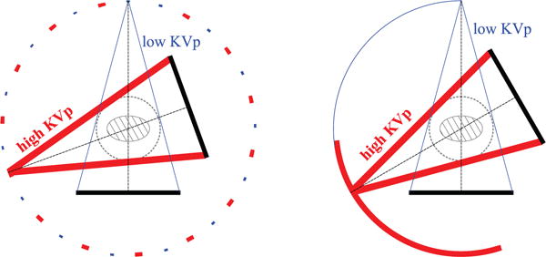
Sparse-view (left) and limited-angular-range (right) configurations. In the former, low-KVp (thin line) and high-KVp (thick line) data are collected at two sets of interlaced sparse views uniformly distributed over 2π, whereas in the latter, low-KVp (thin line) and high-KVp (thick line) data are collected over the two adjacent limited-angular ranges.

Study parameters

In the sparse-view configuration in Figure 9, each of the low- and high-KVp data sets contains 320 views, thus forming a total of 640 projection views. Again, at each view, a linear detector consisting of 1024 bins of 0.39-mm size is used for data collection. Therefore, matrices ${\mathcal{A}}^{[1]}$ and ${\mathcal{A}}^{[2]}$ are of identical dimensions J^[1] = J^[2] = 320×1024 and I = 512 × 512. Furthermore, using the strategy described in Sec. 5.1, we select ε = 0.0116 and 0.008, respectively, for the DE-472- and lung-phantom studies below.

In the limited-angular-range configuration in Figure 9, each of the two adjacent angular ranges covers 98°, thus forming a total of 196°-angular range (corresponding to a short-scan angular range,) and low- or high-KVp data are generated at 174 views uniformly distributed over each of the two angular ranges, respectively, with a linear detector identical to that in the sparse-view configuration. Therefore, matrices ${\mathcal{A}}^{[1]}$ and ${\mathcal{A}}^{[2]}$ are of identical dimensions J^[1] = J^[2] = 174×1024 and I = 512 × 512. Again, using the strategy described in Sec. 5.1, we select ε = 0.0085 and 0.0064, respectively, for the DE-472- and lung-phantom studies below.

Study results

We show in Figure 10 reconstruction results for both phantoms from data acquired with the sparse-view configuration. Reconstructed monochromatic images at 40 and 120 KeV visually resemble their counterparts obtained from the full-scan data. Both basis images of each phantom show clear material separation, and the monochromatic images display an uniform background and no visible artifacts caused by non-linear spectral effect. In addition to reconstruction visualization, we also plot in Figure 11 profiles of the reconstructed and truth monochromatic images along the horizontal and vertical lines indicated in row 2 of Figure 6. It can be observed that for sparse-view-scan configuration, the agreement of monochromatic images reconstructed with the truth counterparts is comparable to that for the full-scan configuration in Figure 7.

Figure 10.

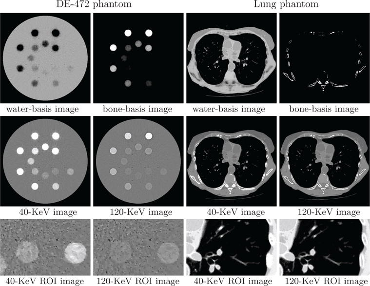
Water- and bone-basis images (row 1), 40- and 120-KeV monochromatic images (row 2), and zoomed-in views of ROI images (row 3) similar to those in row 3 of Figure 6 from sparse-view-scan data of the DE-472 and lung phantoms, respectively, with display windows [0, 1.5] (row 1), [−1000, 1000] HU (row 2), and [−500, 500] HU (row 3, DE-472 phantom) and [−1000, 200] HU (row 3, lung phantom).

Figure 11.

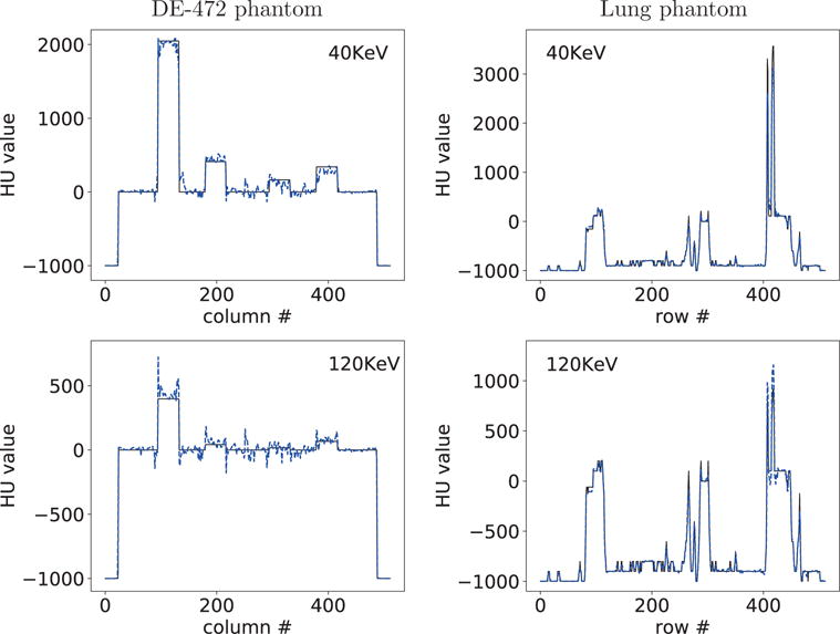
Profiles of reconstructed (dashed) and truth (solid) monochromatic energy images at 40 and 120 KeV along the horizontal and vertical lines indicated in row 2 of Figure 6 from sparse-view-scan data of the DE-472 and lung phantoms, respectively.

We display in Figure 12 reconstruction results for both phantoms from data acquired with the limited-angular-range configurations. Monochromatic image at 40 KeV for the DE-472 phantom shows visible artifacts, due to the poor conditioning of the DD-data model for the limited-angular-range scan considered and the presence of high-concentration calcium and iodine inserts in the phantom, while the monochromatic image at 120 KeV reveals less artifacts. On the other hand, monochromatic images for the lung phantom appear to be with artifacts much less prominent than those for the DE-472 phantom. In addition to reconstruction visualization, we also plot in Figure 13 profiles of the reconstructed and truth monochromatic images along the horizontal and vertical lines indicated in Figure 6, which reveal quantitatively their differences. The lung-phantom reconstructions agree reasonably well with their truths for both energy levels, whereas some differences between the DE-phantom reconstructions and truth counterparts can be observed especially for the limited-angular-range configuration.

Figure 12.

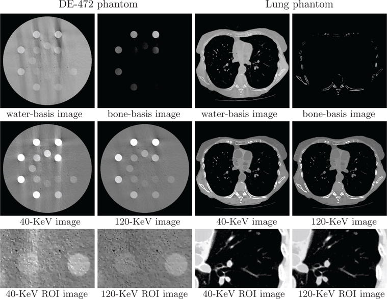
Water- and bone-basis images (row 1), 40- and 120-KeV monochromatic images (row 2), and zoomed-in views of ROI images (row 3) similar to those in row 3 of Figure 6 from limited-angular-range-scan data of the DE-472 and lung phantoms, respectively, with display windows [0, 1.5] (row 1), [−1000, 1000] HU (row 2), and [−500, 500] HU (row 3, DE-472 phantom) and [−1000, 200] HU (row 3, lung phantom).

Figure 13.

Profiles of reconstructed (dashed) and truth (solid) monochromatic images at 40 and 120 KeV along the horizontal and vertical lines indicated in row 2 of Figure 6 from limited-angular-range-scan data of the DE-472 and lung phantoms, respectively.

6.2. Configurations with varying illumination coverages

We consider two additional non-standard configurations, as shown in Figure 14, which involve varying illumination coverage, and are referred to as the split- and block-illumination configurations, respectively. In the configurations, low- and high-KVp data are collected, respectively, with two adjacent and multiple adjacent alternating illumination coverages at each of 640 views uniformly distributed over 2π. The configurations can be achieved through, e.g., the use of a beam blocker in front of the X-ray source and/or detector blocks with different energy responses [38, 39].

Figure 14.

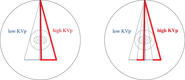
Split- (left) and block-illumination (right) configurations in which low-KVp (thin line) and high-KVp (thick line) data are collected, respectively, with two adjacent and multiple adjacent alternating illumination coverage at each of 640 views uniformly distributed over 2π.

Study parameters

In the split-illumination configuration, the linear detector with 1024 bins (i.e., 400-mm length) is divided into two adjacent segments of equal length with 512 bins (i.e., 200-mm length), as shown in Figure 14, and the low or high KVp beam illuminates one of the two segments, respectively. Therefore, matrices ${\mathcal{A}}^{[1]}$ and ${\mathcal{A}}^{[2]}$ are of identical dimensions J^[1] = J^[2] = 640 × 512 and I = 512 × 512. Using the strategy described in Sec. 5.1, we select ε = 0.0118 and 0.008, respectively, for the DE-472- and lung-phantom studies below.

In the block-illumination configuration, the linear detector is divided into two sets of interlaced, adjacent detector blocks of equal length with 32 bins (i.e., 12.5-mm length), as shown in Figure 14, and the low or high KVp beam illuminates one of the two sets of detector blocks, respectively. Therefore, matrices ${\mathcal{A}}^{[1]}$ and ${\mathcal{A}}^{[2]}$ are of identical dimensions J^[1] = J^[2] = 640 × 512 and I = 512 × 512. Using the strategy described in Sec. 5.1, we select ε = 0.0121 and 0.0089, respectively, for the DE-472- and lung-phantom studies below.

Study results

We show in Figure 15 reconstruction results for both phantoms from data acquired with the split-illumination configuration. Monochromatic image at 40 KeV for the DE-472 phantom show some visible artifacts, while the monochromatic image at 120 KeV reveals less artifacts. Conversely, monochromatic images for the lung phantom appear to reveal little artifacts. In addition to reconstruction visualization, we also plot in Figure 16 profiles of the reconstructed and truth monochromatic images along the horizontal and vertical lines indicated in row 2 of Figure 6. It can be observed that while some quantitative difference between the reconstructed and truth monochromatic images for the DE-472 phantom can be observed, the truth and reconstructed monochromatic images agree reasonably well quantitatively for the lung phantom. In Figures 17 and 18, we display reconstruction results for both phantoms from data acquired with the block-illumination configurations. Based upon the reconstruction results, observations similar to those for the split-illumination configuration can be made.

Figure 15.

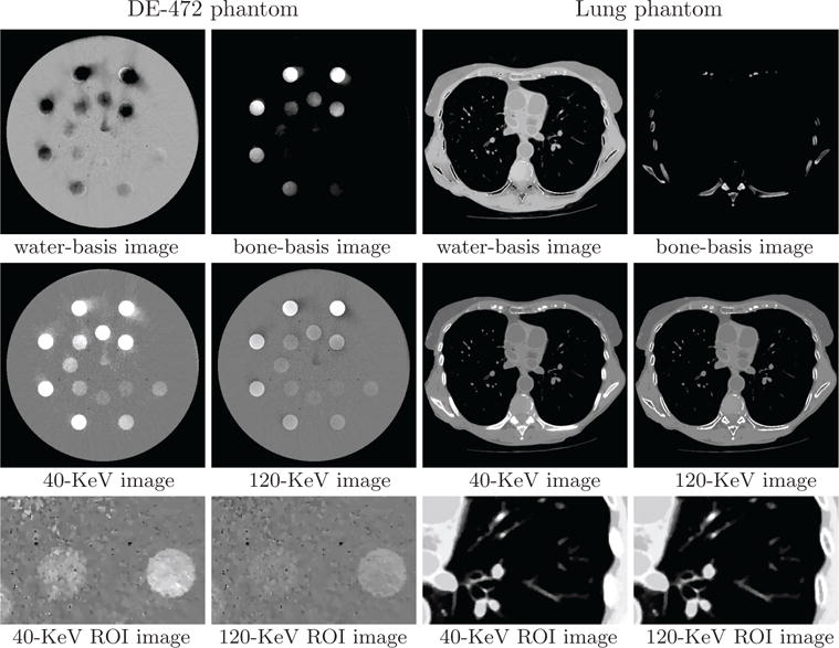
Water- and bone-basis images (row 1), 40- and 120-KeV monochromatic images (row 2), and zoomed-in views of ROI images (row 3) similar to those in row 3 of Figure 6 from split-illumination-scan data of the DE-472 and lung phantoms, respectively, with display windows [0, 1.5] (row 1), [−1000, 1000] HU (row 2), and [−500, 500] HU (row 3, DE-472 phantom) and [−1000, 200] HU (row 3, lung phantom).

Figure 16.

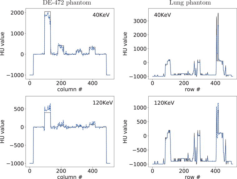
Profiles of reconstructed (dashed) and truth (solid) monochromatic images at 40 and 120 KeV along the horizontal and vertical lines indicated in row 2 of Figure 6 from split-illumination-scan data of the DE-472 and lung phantoms, respectively.

Figure 17.

Water- and bone-basis images (row 1), 40- and 120-KeV monochromatic images (row 2), and zoomed-in views of ROI images (row 3) similar to those in row 3 of Figure 6 from block-illumination-scan data of the DE-472 and lung phantoms, respectively, with display windows [0, 1.5] (row 1), [−1000, 1000] HU (row 2), and [−500, 500] HU (row 3, DE-472 phantom) and [−1000, 200] HU (row 3, lung phantom).

7. Discussion

In the work, we have proposed a one-step, optimization-based approach for image reconstruction in MCT, with an emphasis on demonstrating its potential for enabling scan configurations of potential practical significance. The challenge of optimization-based image reconstruction in MCT stems from its non-linear data model that can lead to a non-convex optimization program for which no mathematically exact solver is available for achieving its globally optimal solution. We have studied a non-convex optimization program, derived its KKT condition, and proposed an algorithm (or procedure) numerically to solve the program for image reconstruction in MCT. A property of the algorithm proposed is that it can reconstruct images in MCT without the requirement of multiple spectral measurements for the same ray. We demonstrate the exploitation of this algorithm property to enable scan configurations of practical interest in terms of potentially lowered hardware cost, enhanced scanning flexibility, and reduced imaging dose/time in MCT.

We have investigated, in addition to the standard, full-scan configuration in MCT, four non-standard configurations with different designs of scanning angular range and illumination coverage each of which acquires only a portion of data of the full-scan configuration. The new configurations are considered because they can readily be implemented on a standard CT scanner employing regular X-ray tubes and energy-integrating detectors without invoking hardware additions and/or modifications to the scanner. The study results suggest that the configurations considered can be enabled by the algorithm proposed to yield monochromatic images comparable to those of the full-scan configuration both visually and quantitatively. While we have demonstrated scan-configuration enabling in dual-energy CT in the work, the algorithm can accommodate multiple (> 2) spectral scans and/or a variety of configurations with different designs of source trajectory and/or illumination coverage tailored to specific applications.

The enabling effectiveness of the algorithm depends upon a number of factors, including sampling conditions and their impact on the data-model conditioning for a specific configuration, appropriateness of spectra used, anatomy complexity of subjects imaged, decomposition error, and data noise. In the presence of data inconsistencies such as decomposition error and statistical noise, some banding artifacts near high contrast structures in DE-472-phantom images are observed to appear stronger understandably for the limited-angular-range configuration than for other configurations, suggesting that the effectiveness of the algorithm in enabling, e.g., a configuration with a considerably limited angular-range, decreases relative to that for other configurations. Conversely, the results show that reconstructions of the lung phantom appear to be robust for the configurations considered.

Without exception, any optimization-based reconstruction would involve some parameters. In the optimization-based reconstruction considered, parameter ε plays a key role in impacting the image reconstruction. We have devised metrics quantitatively to select ε specific to the simulation-data study performed. However, by no means are we suggesting the same metrics for determining ε in realistic, practical applications. Instead, metrics specific to the actual tasks should be designed for the determination of parameter ε in practical applications.

The algorithm derivation relies upon the linearization of the non-linear DD-data model. Because there can be multiple ways different than that used in the work for the linearization, it is of theoretical and practical interest in investigating the impact of different linearization on image reconstruction for various configurations in MCT. We have considered in the work a specific optimization program that includes the data divergence in a ℓ₂-norm form. Different optimization programs can lead to different reconstructions especially in the presence of data inconsistencies such as noise. It would be worthwhile to investigate and prototype optimization programs of different forms (e.g., containing the KL or other data divergences) for enabling scan configurations and obtaining reconstructions of specific application interest [30, 40, 41]. Additional image constraints other than the image-TV constraint can also be incorporated into the programs. For example, appropriate constraints on the basis-image values may be imposed for possibly improving image reconstruction in MCT, especially for the limited-angular-range scan configuration [42].

We recall that the purposes of the work are to investigate the algorithm for image reconstruction and to demonstrate its potential of enabling non-standard configurations of practical implication in MCT. We have performed simulation studies for verifying the design and implementation of the algorithm and for initial demonstration and characterization of the algorithm’s potential for scan-configuration enabling. While the study can hopefully provide insights into the design and implementation of scan configurations of practical interest in MCT, it is not intended to establish and assess the truly application-specific utility of the algorithm proposed and scan configurations enabled. Instead, future works are warranted to investigate, assess, and establish the utility of the algorithm and scan configurations in carefully designed studies with clearly devised task-specific metrics.

Appendix A. Derivation of the local optimality condition

Using equation (1), we can obtain monochromatic energy images as f_n = Σ_k μ_knb_k at N energies, where n = 1, 2,⋯, N. Lower- or upper-bound constraints on the images can be written as

$${\displaystyle \sum _k{\stackrel{\sim }{\mu }}_{kn}{\mathbf{b}}_k+p_n⪰}0\text{for}n=1,2,\cdots ,N,$$ (A.1)

where p_n is a scalar for specifying the upper or lower bound of the nth monochromatic image, and ${\stackrel{\sim }{\mu }}_{kn}=\pm {\mu }_{kn}$ with the negative sign used to impose a lower bound of image values, or simply non-negativity, on the monochromatic images.

We can rewrite equation (A.1) in a linear form of b as

$${\mathcal{Q}}_n\mathbf{b}+{\mathbf{p}}_n⪰0\text{for}n=1,2,\cdots ,N,$$ (A.2)

where

$${\mathcal{Q}}_n=({\stackrel{\sim }{\mu }}_{1n}\mathcal{I},{\stackrel{\sim }{\mu }}_{2n}\mathcal{I},\cdots ,{\stackrel{\sim }{\mu }}_{Kn}\mathcal{I}),$$ (A.3)

and $\mathcal{I}$ denotes the identity matrix of size I × I.

We now consider an optimization program in the form of

$$\mathbf{b}\ast =\underset{\mathbf{b}}{min}\mathrm{\Psi }(\mathbf{b})$$

$$\mathrm{s}.\mathrm{t}.{\mathrm{\Phi }}^2(\mathbf{b};{\mathbf{g}}_{\mathcal{M}})\le {\epsilon }^2,{\mathcal{Q}}_n\mathbf{b}+{\mathbf{p}}_n⪰0\text{for}n=1,2,\cdots ,N.$$ (A.4)

and derive its first-order optimality conditions, i.e., the Karush-Kuhn-Tucker (KKT) conditions. It can readily be shown that the optimzation programs in equations (A.4) and (9) are equivalent when N = K, p_n = 0, and ${\stackrel{\sim }{\mu }}_{kn}=-1$ for k = n (0 otherwise). Therefore, the derived KKT conditions for the former are applicable to the latter.

The Lagrangian of the optimization program in equation (A.4) is given as

$$L(\mathbf{b},\nu ,\{{\mathbf{\lambda }}_n\})=\mathrm{\Psi }(\mathbf{b})+\nu ({\mathrm{\Phi }}^2(\mathbf{b})-{\epsilon }^2)+{\displaystyle \sum _n{\mathbf{\lambda }}_n^{\top }}({\mathcal{Q}}_n\mathbf{b}+{\mathbf{p}}_n),$$ (A.5)

where scalar ν and vectors {λ_n} are the Lagrangian multipliers. The KKT conditions can thus be expressed as

$${\mathrm{\Phi }}^2(\mathbf{b}\ast )\le {\epsilon }^2,$$ (A.6a)

$${\mathcal{Q}}_n\mathbf{b}\ast +{\mathbf{p}}_n⪰0,n=1,2,\cdots ,N,$$ (A.6b)

$$\nu \ast \ge 0,$$ (A.6c)

$${\mathbf{\lambda }}_n^{\ast }⪰0,n=1,2,\cdots ,N,$$ (A.6d)

$${\nabla }_{\mathbf{b}}L(\mathbf{b}\ast ,\nu \ast ,\{{\mathbf{\lambda }}_n^{\ast }\})={\nabla }_{\mathbf{b}}\mathrm{\Psi }(\mathbf{b}\ast )+\nu \ast {\nabla }_{\mathbf{b}}{\mathrm{\Phi }}^2(\mathbf{b}\ast )+{\displaystyle \sum _n{\mathcal{Q}}_n^{\top }}{\mathbf{\lambda }}_n^{\ast }=0,$$ (A.6e)

$$\nu \ast ({\mathrm{\Phi }}^2(\mathbf{b}\ast )-{\epsilon }^2)=0,$$ (A.6f)

$${\mathbf{\lambda }}_n^{\ast \top }({\mathcal{Q}}_n\mathbf{b}\ast +{\mathbf{p}}_n)=0,n=1,2,\cdots ,N,$$ (A.6g)

where b^∗ and $(\nu \ast ,\{{\mathbf{\lambda }}_n^{\ast }\})$ are optimal variables and Lagrangian multipliers for the optimization problem. Given the specific form of ${\mathcal{Q}}_n$ in equation (A.3), the last part of the gradient of the Lagrangian in equation (A.6e) can be simplified as

$${\displaystyle \sum _n{\mathcal{Q}}_n^{\top }{\mathbf{\lambda }}_n^{\ast }=}{\left({\displaystyle \sum _n{\stackrel{\sim }{\mu }}_{1n}{\mathbf{\lambda }}_n^{\ast },}{\displaystyle \sum _n{\stackrel{\sim }{\mu }}_{2n}{\mathbf{\lambda }}_n^{\ast },}\cdots ,{\displaystyle \sum _n{\stackrel{\sim }{\mu }}_{Kn}{\mathbf{\lambda }}_n^{\ast }}\right)}^{\top }.$$ (A.7)

In general, for non-zero ${\stackrel{\sim }{\mu }}_{kn}$, equation (A.7) has zero entries wherever all $\left\{{\mathbf{\lambda }}_n^{\ast }\right\}$ have zeros at the same entries. Based on this observation, we turn to the complementary slackness in (A.6g), which follows

$$\{\begin{array}{cc}{\mathrm{\lambda }}_{ni}^{\ast }=0& \text{if}{({\mathcal{Q}}_n\mathbf{b}\ast )}_i+p_n>0,\\ {\mathrm{\lambda }}_{ni}^{\ast }>0& \text{if}{({\mathcal{Q}}_n\mathbf{b}\ast )}_i+p_n=0.\end{array}$$ (A.8)

We use vector 𝟙_n(b) of size I to denote an identity function, whose elements are

$${⪰}_n\left(\mathbf{b}\right)=\{\begin{array}{cc}1& \text{if}{\left({\mathcal{Q}}_n\mathbf{b}\right)}_i+p_n>0,\\ 0& \text{if}{\left({\mathcal{Q}}_n\mathbf{b}\right)}_i+p_n=0,\end{array}$$ (A.9)

and diag(x) a function that yields a diagonal matrix with the elements of vector x placed along the diagonal line, as

$$\text{diag}(\mathbf{x})=\left(\begin{array}{lllll}{x}_0\hfill & \hfill & \hfill & \hfill & \hfill \\ \hfill & \ddots \hfill & \hfill & \hfill & \hfill \\ \hfill & \hfill & x_i\hfill & \hfill & \hfill \\ \hfill & \hfill & \hfill & \ddots \hfill & \hfill \\ \hfill & \hfill & \hfill & \hfill & x_{I-1}\hfill \end{array}\right).$$ (A.10)

Subsequently, considering all N constraints, we construct a matrix as the product of N diagonal matrices

$$\mathcal{D}(\mathbf{b})={\displaystyle \prod _{n=1}^N\text{diag}({⪰}_n(\mathbf{b}))}.$$ (A.11)

As a result, $\mathcal{D}(\mathbf{b})$ is also diagonal of size I and it picks out those image pixels at which location the N linear constraints in equation (A.1) or (A.2) are strictly satisfied simultaneously. Finally, we use K identical $\mathcal{D}(\mathbf{b})$ and place them in a diagonal line to form a bigger diagonal matrix $\mathcal{D}\prime (\mathbf{b})$ of size I × K as

$$\mathcal{D}\prime (\mathbf{b})=\left(\begin{array}{lll}\mathcal{D}(\mathbf{b})\hfill & \hfill & \hfill \\ \hfill & \ddots \hfill & \hfill \\ \hfill & \hfill & \mathcal{D}(\mathbf{b})\hfill \end{array}\right).$$ (A.12)

Given the meaning of $\mathcal{D}(\mathbf{b})$ as described above, left-multiplying $\mathcal{D}\prime (\mathbf{b}\ast )$ to both sides of equations (A.7) yields

$$\mathcal{D}\prime (\mathbf{b}\ast ){\displaystyle \sum _n{\mathcal{Q}}_n^{\top }}{\mathbf{\lambda }}_n^{\ast }={\left(\mathcal{D}(\mathbf{b}\ast ){\displaystyle \sum _n{\stackrel{\sim }{\mu }}_{1n}{\mathbf{\lambda }}_n^{\ast }},\mathcal{D}(\mathbf{b}\ast ){\displaystyle \sum _n{\stackrel{\sim }{\mu }}_{2n}{\mathbf{\lambda }}_n^{\ast }},\cdots ,\mathcal{D}(\mathbf{b}\ast ){\displaystyle \sum _n{\stackrel{\sim }{\mu }}_{Kn}{\mathbf{\lambda }}_n^{\ast }}\right)}^{\top }=0.$$

We can simplify the first order optimality condition in equation (A.6e) as

$${\mathbf{d}}_{\text{TV}}(\mathbf{b}\ast )+{\mathbf{d}}_{\text{data}}(\mathbf{b}\ast )=0,$$ (A.13)

where

$${\mathbf{d}}_{\text{TV}}(\mathbf{b}\ast )=\mathcal{D}\prime (\mathbf{b}\ast ){\nabla }_{\mathbf{b}}\mathrm{\Psi }(\mathbf{b}\ast )$$

and

$${\mathbf{d}}_{\text{data}}(\mathbf{b}\ast )=\nu \ast \mathcal{D}\prime (\mathbf{b}\ast ){\nabla }_{\mathbf{b}}{\mathrm{\Phi }}^2(\mathbf{b}\ast ).$$

Now equation (A.6c) states that ν* is non-negative (dual feasibility), and the complementary slackness in (A.6f) states that ν* can only be zero when the data fidelity constraint is not active. For practical solutions that are non-trivial, i.e., other than non-negative flat images, the data fidelity constraint is always active. Therefore, it is desired that ν* > 0 in practical situations, which leads to that d_TV(b*) and d_data(b*) shall be oppositely co-linear, or

$$c_{\alpha }\equiv {\widehat{\mathbf{d}}}_{\text{TV}}^{\top }({\mathbf{b}}^{\ast }){\widehat{\mathbf{d}}}_{\text{data}}({\mathbf{b}}^{\ast })=-1,$$ (A.14)

where ${\widehat{\mathbf{d}}}_{\text{TV}}({\mathbf{b}}^{\ast })={\mathbf{d}}_{\text{TV}}({\mathbf{b}}^{\ast })/|{\mathbf{d}}_{\text{TV}}({\mathbf{b}}^{\ast })|$ and ${\widehat{\mathbf{d}}}_{\text{data}}({\mathbf{b}}^{\ast })={\mathbf{d}}_{\text{data}}({\mathbf{b}}^{\ast })/|{\mathbf{d}}_{\text{data}}({\mathbf{b}}^{\ast })|$ are the normalized vectors.

For computing d_TV(b*), using Ψ(b) in equation (10), we have

$${\nabla }_{\mathbf{b}}\mathrm{\Psi }({\mathbf{b}}^{\ast })={\displaystyle \sum _k{\nabla }_{\mathbf{b}}\Vert {\mathbf{b}}_k^{\ast }{\Vert }_{\text{TV}}},$$ (A.15)

where

$${\nabla }_{\mathbf{b}}\Vert {\mathbf{b}}_k^{\ast }{\Vert }_{\text{TV}}=\{\begin{array}{ll}{\nabla }_{b_i}\Vert {\mathbf{b}}_k^{\ast }{\Vert }_{\text{TV}}\hfill & \text{if }{b}_i\in {\mathbf{b}}_k,\hfill \\ 0\hfill & \text{if }{b}_i\cancel{\in }{\mathbf{b}}_k.\hfill \end{array}$$

As the ℓ₁-norm function is non-smooth, TV gradients, or ${\nabla }_{{\mathbf{b}}_k}\Vert {\mathbf{b}}_k^{\ast }{\Vert }_{\text{TV}}$, are computed based on an approximation of a smoothed version [43].

On the other hand, for computing d_data(b*), we have

$${\mathrm{\Phi }}^2(\mathbf{b})={({\mathbf{g}}_{\mathcal{M}}^{\top }{\mathbf{g}}_{\mathcal{M}})}^{-1}{(\mathbf{g}(\mathbf{b})-{\mathbf{g}}_{\mathcal{M}})}^{\top }(\mathbf{g}(\mathbf{b})-{\mathbf{g}}_{\mathcal{M}}).$$ (A.16)

Taking its gradient yields

$${\nabla }_{\mathbf{b}}{\mathrm{\Phi }}^2(\mathbf{b})=2{({\mathbf{g}}_{\mathcal{M}}^{\top }{\mathbf{g}}_{\mathcal{M}})}^{-1}J(\mathbf{g}(\mathbf{b}),\mathbf{b})(\mathbf{g}(\mathbf{b})-{\mathbf{g}}_{\mathcal{M}}),$$ (A.17)

where Jacobian matrix J(y(x), x) is given by

$$J(\mathbf{y}(\mathbf{x}),\mathbf{x})=\left(\begin{array}{ccc}\frac{\partial y{(\mathbf{x})}_1}{\partial x_1}& \frac{\partial y{(\mathbf{x})}_2}{\partial x_1}& \cdots \\ \frac{\partial y{(\mathbf{x})}_1}{\partial x_2}& \frac{\partial y{(\mathbf{x})}_2}{\partial x_2}& \cdots \\ ⋮& ⋮& \ddots \end{array}\right),$$ (A.18)

where y(x)_j and x_i are the j-th and i-th elements of vectors y(x) and x, respectively. Given the concatenated form of the aggregate basis image vector as $\mathbf{b}={({\mathbf{b}}_1^{\top },{\mathbf{b}}_2^{\top },\cdots ,{\mathbf{b}}_K^{\top })}^{\top }$ and the dimension of vector g(b) being $J^{\prime }\equiv {\displaystyle {\sum }_s{J}^{[s]}}$, where J^[s] is the size of data vector g^[s](b) for spectral set s, the Jacobian in equation (A.17) can be re-expressed as

$$J(\mathbf{g}(\mathbf{b}),\mathbf{b})=\left(\begin{array}{cccc}{\nabla }_{{\mathbf{b}}_1}g{(\mathbf{b})}_1,& {\nabla }_{{\mathbf{b}}_1}g{(\mathbf{b})}_2,& \cdots & {\nabla }_{{\mathbf{b}}_1}g{(\mathbf{b})}_{J^{\prime }},\\ {\nabla }_{{\mathbf{b}}_2}g{(\mathbf{b})}_1,& {\nabla }_{{\mathbf{b}}_2}g{(\mathbf{b})}_2,& \cdots & {\nabla }_{{\mathbf{b}}_2}g{(\mathbf{b})}_{J^{\prime }},\\ ⋮& ⋮& \ddots & ⋮\\ {\nabla }_{{\mathbf{b}}_K}g{(\mathbf{b})}_1,& {\nabla }_{{\mathbf{b}}_K}g{(\mathbf{b})}_2,& \cdots & {\nabla }_{{\mathbf{b}}_K}g{(\mathbf{b})}_{J^{\prime }},\end{array}\right).$$ (A.19)

Recall equation (8), where the element of data vector g(b) may depend upon spectral set index s and ray index j. In this derivation, instead, a single index j′ is used for the aggregate data vector g(b), as j′ = j + (s − 1) × J^[s−1] and

$$g_{j^{\prime }}(\mathbf{b})=g_j^{[s]}(\mathbf{b})=-\ln {\displaystyle \sum _m{q}_{jm}^{[s]}\exp }\left(-{\displaystyle \sum _k{\mu }_{km}}{\mathbf{a}}_j^{[s]}{\mathbf{b}}_k\right),$$ (A.20)

As a result, the gradient of $g_{j^{\prime }}(\mathbf{b})$ w.r.t. basis image b_k can be written as

$${\nabla }_{{\mathbf{b}}_k}{g}_{j^{\prime }}(\mathbf{b})={\left({\displaystyle \sum _m{t}_{j^{\prime }m}}\right)}^{-1}\left({\displaystyle \sum _m{\mu }_{km}{t}_{j^{\prime }m}}\right){\mathbf{a}}_{j^{\prime }}^{\top },$$ (A.21)

where

$$t_{j^{\prime }m}=q_{jm}^{[s]}\exp \left(-{\displaystyle \sum _k{\mu }_{km}{\mathbf{a}}_j^{[s]}{\mathbf{b}}_k}\right),{\mathbf{a}}_{j^{\prime }}={\mathbf{a}}_j^{[s]}.$$ (A.22)

Finally, replacing equations (A.19) and (A.21) into equation (A.17) yields

$${\nabla }_{\mathbf{b}}{\mathrm{\Phi }}^2(\mathbf{b})=2{({\mathbf{g}}_{\mathcal{M}}^{\top }{\mathbf{g}}_{\mathcal{M}})}^{-1}J(\mathbf{g}(\mathbf{b}),\mathbf{b})(\mathbf{g}(\mathbf{b})-{\mathbf{g}}_{\mathcal{M}})=\frac{2}{{\mathbf{g}}_{\mathcal{M}}^{\top }{g}_{\mathcal{M}}}\left(\begin{array}{c}{\displaystyle \sum _{j^{\prime }}(g_{j^{\prime }}-g_{\mathcal{M}{j}^{\prime }}){\nabla }_{{\mathbf{b}}_1}{g}_{j^{\prime }}}\\ {\displaystyle \sum _{j^{\prime }}(g_{j^{\prime }}-g_{\mathcal{M}{j}^{\prime }}){\nabla }_{{\mathbf{b}}_2}{g}_{j^{\prime }}}\\ ⋮\\ {\displaystyle \sum _{j^{\prime }}(g_{j^{\prime }}-g_{\mathcal{M}{j}^{\prime }}){\nabla }_{{\mathbf{b}}_K}{g}_{j^{\prime }}}\end{array}\right)=\frac{2}{{\mathbf{g}}_{\mathcal{M}}^{\top }{g}_{\mathcal{M}}}\left(\begin{array}{c}{\displaystyle \sum _{j^{\prime }}\frac{(g_{j^{\prime }}-g_{\mathcal{M}{j}^{\prime }}){\displaystyle \sum _m{\mu }_{1m}^{\prime }{t}_{j^{\prime }m}}}{{\displaystyle \sum _m{t}_{j^{\prime }m}}}{\mathbf{a}}_{j^{\prime }}^{\top }}\\ {\displaystyle \sum _{j^{\prime }}\frac{(g_{j^{\prime }}-g_{\mathcal{M}{j}^{\prime }}){\displaystyle \sum _m{\mu }_{2m}^{\prime }{t}_{j^{\prime }m}}}{{\displaystyle \sum _m{t}_{j^{\prime }m}}}{\mathbf{a}}_{j^{\prime }}^{\top }}\\ ⋮\\ {\displaystyle \sum _{j^{\prime }}\frac{(g_{j^{\prime }}-g_{\mathcal{M}{j}^{\prime }}){\displaystyle \sum _m{\mu }_{Km}^{\prime }{t}_{j^{\prime }m}}}{{\displaystyle \sum _m{t}_{j^{\prime }m}}}{\mathbf{a}}_{j^{\prime }}^{\top }}\end{array}\right).$$ (A.23)

References

- 1.Carmi R, Naveh G, Altman A. Material separation with dual-layer CT. 2005 IEEE Nuclear Science Symposium Conference Record. 2005 Oct;4:1876–1878. [Google Scholar]
- 2.Flohr TG, McCollough CH, Bruder H, Petersilka M, Gruber K, S C, Grasruck M, Stierstorfer K, Krauss B, Raupach R, Primak AN, Kttner A, Achenbach S, Becker C, Kopp A, Ohnesorge BM. First performance evaluation of a dual-source CT (DSCT) system. European Radiology. 2005 Dec;16(2):256–268. doi: 10.1007/s00330-005-2919-2. [Online]. Available: http://link.springer.com/article/10.1007/s00330-005-2919-2. [DOI] [PubMed] [Google Scholar]
- 3.Johnson TRC, Krau B, Sedlmair M, Grasruck M, Bruder H, Morhard D, Fink C, Weckbach S, Lenhard M, Schmidt B, Flohr T, Reiser MF, Becker CR. Material differentiation by dual energy CT: Initial experience. European Radiology. 2007 Jun;17(6):1510–1517. doi: 10.1007/s00330-006-0517-6. https://link.springer.com/article/10.1007/s00330-006-0517-6. [DOI] [PubMed] [Google Scholar]
- 4.Roessl E, Proksa R. K-edge imaging in X-ray computed tomography using multi-bin photon counting detectors. Physics in Medicine and Biology. 2007;52(15):4679. doi: 10.1088/0031-9155/52/15/020. [Online]. Available: http://stacks.iop.org/0031-9155/52/i=15/a=020. [DOI] [PubMed] [Google Scholar]
- 5.Schlomka JP, Roessl E, Dorscheid R, Dill S, Martens G, Istel T, Bumer C, Herrmann C, Steadman R, Zeitler G, Livne A, Proksa R. Experimental feasibility of multi-energy photon-counting K-edge imaging in pre-clinical computed tomography. Physics in Medicine and Biology. 2008;53(15):4031. doi: 10.1088/0031-9155/53/15/002. [Online]. Available: http://stacks.iop.org/0031-9155/53/i=15/a=002. [DOI] [PubMed] [Google Scholar]
- 6.Xu D, Langan DA, Wu X, Pack JD, Benson TM, Tkaczky JE, Schmitz AM. Dual energy CT via fast kVp switching spectrum estimation. Proc SPIE, Medical Imaging: Physics of Medical Imaging. 2009;7258:72 583T–72 583T–10. [Online]. Available: http://dx.doi.org/10.1117/12.811650. [Google Scholar]
- 7.Taguchi K, Iwanczyk JS. Vision 20/20: Single photon counting x-ray detectors in medical imaging. Medical Physics. 2013 Oct;40(10) doi: 10.1118/1.4820371. [Online]. Available: http://www.ncbi.nlm.nih.gov/pmc/articles/PMC3786515/ [DOI] [PMC free article] [PubMed] [Google Scholar]
- 8.Primak AN, Fletcher JG, Vrtiska TJ, Dzyubak OP, Lieske JC, Jackson ME, Williams J, Jr, McCollough CH. Noninvasive differentiation of uric acid versus nonuric acid kidney stones using dual-energy CT. Academic Radiology. 2007 Dec;14(12):1441–1447. doi: 10.1016/j.acra.2007.09.016. http://www.sciencedirect.com/science/article/pii/S1076633207005235. [DOI] [PMC free article] [PubMed] [Google Scholar]
- 9.Thieme SF, Becker CR, Hacker M, Nikolaou K, Reiser MF, Johnson TRC. Dual energy CT for the assessment of lung perfusion correlation to scintigraphy. European Journal of Radiology. 2008 Dec;68(3):369–374. doi: 10.1016/j.ejrad.2008.07.031. http://www.sciencedirect.com/science/article/pii/S0720048X08004415. [DOI] [PubMed] [Google Scholar]
- 10.Graser A, Johnson TRC, Chandarana H, Macari M. Dual energy CT: preliminary observations and potential clinical applications in the abdomen. European Radiology. 2009 Jan;19(1):13. doi: 10.1007/s00330-008-1122-7. [Online]. Available: https://link.springer.com/article/10.1007/s00330-008-1122-7. [DOI] [PubMed] [Google Scholar]
- 11.McCollough CH, Leng S, Yu L, Fletcher JG. Dual- and multi-energy CT: principles, technical approaches, and clinical applications. Radiology. 2015 Aug;276(3):637–653. doi: 10.1148/radiol.2015142631. http://pubs.rsna.org/doi/abs/10.1148/radiol.2015142631. [DOI] [PMC free article] [PubMed] [Google Scholar]
- 12.Pourmorteza A, Symons R, Sandfort V, Mallek M, Fuld MK, Henderson G, Jones EC, Malayeri AA, Folio LR, Bluemke DA. Abdominal imaging with contrast-enhanced photon-counting CT: First human experience. Radiology. 2016 Feb;:152601. doi: 10.1148/radiol.2016152601. [Online]. Available: http://pubs.rsna.org/doi/10.1148/radiol.2016152601. [DOI] [PMC free article] [PubMed]
- 13.Alvarez RE, Macovski A. Energy-selective reconstructions in X-ray computerised tomography. Physics in Medicine and Biology. 1976;21(5):733. doi: 10.1088/0031-9155/21/5/002. [Online]. Available: http://stacks.iop.org/0031-9155/21/i=5/a=002. [DOI] [PubMed] [Google Scholar]
- 14.Zou Y, Silver MD. Analysis of fast kV-switching in dual energy CT using a pre-reconstruction decomposition technique. Proc SPIE, Medical Imaging: Physics of Medical Imaging. 2008;6913:691 313–691 313–12. [Online]. Available: http://dx.doi.org/10.1117/12.772826. [Google Scholar]
- 15.Sawatzky A, Xu Q, Schirra C, Anastasio M. Proximal ADMM for multi-channel image reconstruction in spectral X-ray CT. IEEE Transactions on Medical Imaging. 2014 Aug;33(8):1657–1668. doi: 10.1109/TMI.2014.2321098. [DOI] [PubMed] [Google Scholar]
- 16.Rigie DS, LaRiviere PJ. Joint reconstruction of multi-channel, spectral CT data via constrained total nuclear variation minimization. Physics in Medicine and Biology. 2015 Mar;60(5):1741. doi: 10.1088/0031-9155/60/5/1741. [Online]. Available: http://iopscience.iop.org/0031-9155/60/5/1741. [DOI] [PMC free article] [PubMed] [Google Scholar]
- 17.Brooks RA. A quantitative theory of the Hounsfield unit and its application to dual energy scanning. Journal of Computer Assisted Tomography. 1977 Oct;1(4):487–493. doi: 10.1097/00004728-197710000-00016. [DOI] [PubMed] [Google Scholar]
- 18.Maass C, Baer M, Kachelriess M. Image-based dual energy CT using optimized precorrection functions: A practical new approach of material decomposition in image domain. Medical Physics. 2009 Aug;36(8):3818–3829. doi: 10.1118/1.3157235. http://scitation.aip.org/content/aapm/journal/medphys/36/8/10.1118/1.3157235. [DOI] [PubMed] [Google Scholar]
- 19.Mendonca PRS, Lamb P, Sahani DV. A flexible method for multi-material decomposition of dual-energy CT images. IEEE Transactions on Medical Imaging. 2014 Jan;33(1):99–116. doi: 10.1109/TMI.2013.2281719. http://ieeexplore.ieee.org/lpdocs/epic03/wrapper.htm?arnumber=6600785. [DOI] [PubMed] [Google Scholar]
- 20.Elbakri I, Fessler J. Statistical image reconstruction for polyenergetic X-ray computed tomography. IEEE Transactions on Medical Imaging. 2002 Feb;21(2):89–99. doi: 10.1109/42.993128. [DOI] [PubMed] [Google Scholar]
- 21.Cai C, Rodet T, Legoupil S, Mohammad-Djafari A. A full-spectral Bayesian reconstruction approach based on the material decomposition model applied in dual-energy computed tomography. Medical Physics. 2013 Nov;40(11):n/a–n/a. doi: 10.1118/1.4820478. [Online]. Available: http://onlinelibrary.wiley.com/doi/10.1118/1.4820478/abstract. [DOI] [PubMed] [Google Scholar]
- 22.Long Y, Fessler J. Multi-material decomposition using statistical image reconstruction for spectral CT. IEEE Transactions on Medical Imaging. 2014 Aug;33(8):1614–1626. doi: 10.1109/TMI.2014.2320284. [DOI] [PMC free article] [PubMed] [Google Scholar]
- 23.Zhang R, Thibault JB, Bouman C, Sauer K, Hsieh J. Model-based iterative reconstruction for dual-energy X-ray CT using a joint quadratic likelihood model. IEEE Transactions on Medical Imaging. 2014 Jan;33(1):117–134. doi: 10.1109/TMI.2013.2282370. [DOI] [PubMed] [Google Scholar]
- 24.Nakada K, Taguchi K, Fung GSK, Amaya K. Joint estimation of tissue types and linear attenuation coefficients for photon counting CT. Medical Physics. 2015 Sep;42(9):5329–5341. doi: 10.1118/1.4927261. http://onlinelibrary.wiley.com/doi/10.1118/1.4927261/abstract. [DOI] [PubMed] [Google Scholar]
- 25.Zhao Y, Zhao X, Zhang P. An extended algebraic reconstruction technique (E-ART) for dual spectral CT. IEEE Transactions on Medical Imaging. 2015 Mar;34(3):761–768. doi: 10.1109/TMI.2014.2373396. [DOI] [PubMed] [Google Scholar]
- 26.Barber RF, Sidky EY, Schmidt TG, Pan X. An algorithm for constrained one-step inversion of spectral CT data. Physics in Medicine and Biology. 2016;61(10):3784. doi: 10.1088/0031-9155/61/10/3784. [Online]. Available: http://stacks.iop.org/0031-9155/61/i=10/a=3784. [DOI] [PMC free article] [PubMed] [Google Scholar]
- 27.Natterer F. 2. The Radon Transform and Related Transforms. (Classics in Applied Mathematics Society for Industrial and Applied Mathematics).The Mathematics of Computerized Tomography. 2001 Jan;:9–53. doi: 10.1137/1.9780898719284.ch2. [Online]. Available: http://epubs.siam.org/doi/abs/10.1137/1.9780898719284.ch2. [DOI]
- 28.Pan X, Chen B, Zhang Z, Pearson E, Sidky E, Han X. Optimization-based Reconstruction Exploiting Spectral Information in CT. The Third International Conference on Image Formation in X-Ray Computed Tomography. 2014:228–232. [Google Scholar]
- 29.Sidky EY, Pan X. Image reconstruction in circular cone-beam computed tomography by constrained, total-variation minimization. Physics in Medicine and Biology. 2008;53(17):4777. doi: 10.1088/0031-9155/53/17/021. [Online]. Available: http://stacks.iop.org/0031-9155/53/i=17/a=021. [DOI] [PMC free article] [PubMed] [Google Scholar]
- 30.Sidky EY, Jorgensen JH, Pan X. Convex optimization problem prototyping for image reconstruction in computed tomography with the Chambolle-Pock algorithm. Physics in Medicine and Biology. 2012;57(10):3065. doi: 10.1088/0031-9155/57/10/3065. [Online]. Available: http://stacks.iop.org/0031-9155/57/i=10/a=3065. [DOI] [PMC free article] [PubMed] [Google Scholar]
- 31.Ramani S, Fessler JA. A splitting-based iterative algorithm for accelerated statistical X-ray CT reconstruction. IEEE Transactions on Medical Imaging. 2012 Mar;31(3):677–688. doi: 10.1109/TMI.2011.2175233. [DOI] [PMC free article] [PubMed] [Google Scholar]
- 32.Bian J, Siewerdsen JH, Han X, Sidky EY, Prince JL, Pelizzari CA, Pan X. Evaluation of sparse-view reconstruction from flat-panel-detector cone-beam CT. Physics in Medicine and Biology. 2010;55(22):6575. doi: 10.1088/0031-9155/55/22/001. [Online]. Available: http://stacks.iop.org/0031-9155/55/i=22/a=001. [DOI] [PMC free article] [PubMed] [Google Scholar]
- 33.Hernandez AM, Boone JM. Tungsten anode spectral model using interpolating cubic splines: Unfiltered xray spectra from 20 kV to 640 kV. Medical Physics. 2014 Apr;41(4):042 101–1–042 101–15. doi: 10.1118/1.4866216. [Online]. Available: http://onlinelibrary.wiley.com/doi/10.1118/1.4866216/abstract. [DOI] [PMC free article] [PubMed] [Google Scholar]
- 34.JRTAssociates. Dual energy CT phantom - JRT Associates. 2015 [Online]. Available: http://jrtassociates.com/pdfs/472_DECTPhantom2.pdf.
- 35.Hubbell J, Seltzer S. Tables of X-ray mass attenuation coefficients and mass energy-absorption coefficients (version 1.4) 2004 [Online]. Available: http://physics.nist.gov/xaamdi.
- 36.Berger M, Hubbell J, Seltzer S, Chang J, Coursey J, Sukumar R, Zucker D, Olsen K. XCOM: Photon cross section database (version 1.5) 2010 [Online]. Available: http://physics.nist.gov/xcom.
- 37.Han X, Bian J, Eaker D, Kline T, Sidky E, Ritman E, Pan X. Algorithm-Enabled Low-Dose Micro-CT Imaging. IEEE Transactions on Medical Imaging. 2011 Mar;30(3):606–620. doi: 10.1109/TMI.2010.2089695. [DOI] [PMC free article] [PubMed] [Google Scholar]
- 38.Niu T, Zhu L. Scatter correction for full-fan volumetric CT using a stationary beam blocker in a single full scan. Medical Physics. 2011 Nov;38(11):6027–6038. doi: 10.1118/1.3651619. http://onlinelibrary.wiley.com/doi/10.1118/1.3651619/abstract. [DOI] [PMC free article] [PubMed] [Google Scholar]
- 39.Lee H, Xing L, Lee R, Fahimian BP. Scatter correction in cone-beam CT via a half beam blocker technique allowing simultaneous acquisition of scatter and image information. Medical Physics. 2012 May;39(5):2386–2395. doi: 10.1118/1.3691901. [Online]. Available: http://onlinelibrary.wiley.com/doi/10.1118/1.3691901/abstract. [DOI] [PubMed] [Google Scholar]
- 40.Chambolle A, Pock T. A first-order primal-dual algorithm for convex problems with applications to imaging. Journal of Mathematical Imaging and Vision. 2010 Dec;40(1):120–145. http://link.springer.com/article/10.1007/s10851-010-0251-1. [Google Scholar]
- 41.Zhang Z, Han X, Pearson E, Pelizzari C, Sidky EY, Pan X. Artifact reduction in short-scan CBCT by use of optimization-based reconstruction. Physics in Medicine and Biology. 2016;61(9):3387. doi: 10.1088/0031-9155/61/9/3387. [Online]. Available: http://stacks.iop.org/0031-9155/61/i=9/a=3387. [DOI] [PMC free article] [PubMed] [Google Scholar]
- 42.Chen B, Zhang Z, Pearson E, Sidky E, Pan X. An investigation of regularization for basis image reconstruction in spectral CT; 2015 IEEE Nuclear Science Symposium and Medical Imaging Conference (NSS/MIC); Oct, 2015. pp. 1–3. [Google Scholar]
- 43.Sidky EY, Kao CM, Pan X. Accurate image reconstruction from few-views and limited-angle data in divergent-beam CT. Journal of X-Ray Science and Technology. 2006 Jan;14(2):119–139. http://content.iospress.com/articles/journal-of-x-ray-science-and-technology/xst00155. [Google Scholar]