Detecting causality from short time-series data based on prediction of topologically equivalent attractors

Background

How to correctly detect the causality from the observed time-series is quite important but it is usually very difficult, and has attracted much attention in complex systems in recent years. There are many effective method to infer the causal relation between the variables, such as mutual prediction method [1], state space method [2], phase mode ling method [3], quantifying information method [4], recurrence plots method [5], convergent cross mapping method [6] and so on. As the primary framework, Granger causality (GC) is recognized as one of the most popular measures to reveal causality influence of time-series on the causation problem.

GC can be roughly stated as follows [7]: the variable X was said to “Granger cause” Y if the predictability of Y declines when X was removed from the universe of all possible causative variables u. The key characteristic of GC is separability, which means that the information for a causative factor only depends on one variable. In other words, if the variable X is removed, its information will be eliminated at the same time. However, the assumption of separability is mainly appropriate to the stochastic systems or linear systems because the separability implies that the system is just considered as a part not a whole at one time. Generally, for a linear system with strongly coupled variables, GC is a very powerful tool to detect their interactions. However, it lacks ability to detect the causal relation on weakly coupled variables or nonlinearly coupled variables, in particular for a deterministic system, i.e., for those systems, GC may give ambiguous results or even wrong conclusions.

In order to overcome these drawbacks or shortages, Sugihara et al. [6] proposed a method called convergent cross mapping (CCM) based on the embedded attractor reconstruction. To identify the causal relations between nonlinearly coupled variables or weakly coupled variables, CCM has been shown to have significant advantages over GC, vector autoregression (VAR) [8], conditional mutual information (CMI) [4, 9, 10] and spectral methods [11, 12]. For the topic of causality detection, Hirata et al. [5] also used the recurrence plots method to identify hidden common causes from bivariate time-series, in which a nonconvergent property of a recurrence plot was exploited to deny the existence of causal relation between the bivariate time-series. On the other hand, Hempel et al. [13] proposed and analyzed the inner composition alignment (IOTA) which was permutation-based asymmetric association measure to infer the direction of couplings and indirect links from short time-series. Ma et al. [14] proposed cross map smoothness (CMS) methd to detecting causality with short time series. Runge et al. [15] used the multivariate transfer entropy (TE) method to detect causalities in multivariate time-series. This method can distinguish direct from indirect causality and also identify common drivers. However, it is mainly designed for low dimensional systems. To overcome this limitation, the decomposed transfer entropy was proposed by the same group. Similarly, Runge et al. [16] developed a time-delayed conditional mutual information approach, which is called as momentary information transfer (MIT) and has a well interpretable notion to measure the coupling strength.

The CCM method and many other methods are effective for identifying the causal associations from the observed data, and in particular, CCM method can be thought as another milestone after the GC method to detect causality. However, in spite of those impressive advances on this area, most existing approaches including CCM and GC methods, generally need a long time-series to detect the causal relation, for example, more than 3000 in CCM study. But in many real-world application data, especially in biological systems, the oberved or obtained time-series data (or samples) is usually very short (e.g., sometimes only a few time points). Since these data or samples are highly depended on the experiment or the limited resource. Thus, one natural question is how to detect the causality of these high dimensional short time-series, including those weakly coupled and nonlinearly coupled relations.

In this work, to answer this question, we aim to find an effective method to detect causal relation for high dimensional short time-series or small samples. In other words, in this paper, we propose a new method called topologically equivalent position method shorting for TEP which can detect causality for very short time-series data or small samples. This method is mainly based on attractor embedding theory in nonlinear dynamical systems. Specifically, we exploit the information from the embedding theorem, i.e., two attractors reconstructed from two different observed variables are topological equivalent. That information is used to predict time-series of one variable from another or detect the causality between them based on the principle of topologically equivalent position, i.e., the positions of two corresponding points in the two attractors are topologically equivalent. This prediction can be achieved even by a small number of samples or short time-series. We use both numerical examples and real gene expression data to show the effectiveness of our method. As a result, it shows our method can be effectively used in biological systems. And it can extend GC and CCM methods to general cases. In addition, the comparison studies for different approaches are also provided to show the superiority of our method.

Methods

The definition of causality

In dynamical systems theory, the necessary condition that two variables (time-series) are causally linked each other, is that these two variables are from the same dynamical system or they must share the same attractor. This also means that time-series data of one variable contains the information of other variables in the same system or attractor, and thus can be used to predict the dynamics of other variables. Here the attractor means a set of numerical values of the state invariant under the dynamics or the numerical values toward to a system in the course dynamic evolution. Furthermore, according to the Takens’ delay embedding theorem [17], one can use the observed time-series of one variable to reconstruct the original high-dimensional dynamical behavior by lagged-coordinate [18]. In other words, Takens’ delay embedding theorem grantees that data of each variable can reconstruct the attractor of the original (high dimensional) system. Takens’ embedding theorem provides the theoretical foundation for autonomous dynamical systems with noise-free. However, this is not the case in many real systems. Therefore, Stark et al. [19, 20] extend Takens’ embedding theorem to deterministically forced systems (i.e., non-autonomous system) and further they gave the delay embedding theorems for arbitrarily and stochastically forced systems.

In this paper, based on the lagged-coordinate delay embedding theorem, we develop an effective method to detect the causal relation between a pair of variables (i.e.,genes) for short gene expression data. Specifically, first we define the causality, which is actually a prediction-based concept in this work. We denote the shared common attractor (original attractor in Fig. 1a) as M and the reconstructed attractors by lagged-coordinates from their components, for example, X, Y as M _X, M _Y, respectively (Fig. 1a). Based on the embedding theorem, the reconstructed attractors M _X and M _Y are topologically equivalent.

Fig. 1.

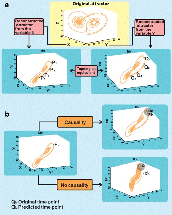
Definition of causality. a. the attractors M _X and M _Y are reconstructed from variables X and Y by lagged-coordinates and they are topological equivalent. b. The predicted time-series (points) $Q_k^{\prime }\left(k=1,2,\cdots \right)$ are located in the nearest neighborhood of Q _k (k = 1, 2, ⋯) which implies causality (see the above part). The predicted time-series (points) $Q_k^{\prime }\left(k=1,2,\cdots \right)$ are outside the nearest neighborhood of Q _k (k = 1, 2, ⋯) which implies no causality (see the below part). Here, the nearest neighborhood is measured by a ball with a small radius r (see the gray district)

The variable Y causes the variable X if and only if one can use the information of X to predict the variable of Y. Taking Fig. 1b for example, two time-series variables {P _i}, (i = 1, 2, ⋯) and {Q _i}, (i = 1, 2, ⋯) are located on their corresponding reconstructed attractors M _X and M _Y, i.e. P _i ∈ M _X, Q _i ∈ M _Y, (i = 1, 2, ⋯). Now we use the information of P _i (i = 1, 2, ⋯) to predict Q _i (i = 1, 2, ⋯), if the predicted time-series (samples) ${\overline{Q}}_i\left(i=1,2,\cdots \right)$ are in the near neighborhood of Q _i (i = 1, 2, ⋯) on attractor M _Y, we call that Y causes X (see Fig. 1b). Otherwise, if the predicted time-series (points) $Q_i^{\prime }\left(i=1,2,\cdots \right)$ are outside the near neighborhood of Q _i (i = 1, 2, ⋯),we say that Y does not cause X (see Fig. 1b). Clearly, such causality is based on the prediction of one variable from data of another variable, and thereby it is the prediction-based causality.

Topologically equivalent position method

To detect the causality between time-series variables, we propose a new method which we call it topologically equivalent position method shorting for TEP. We will use this method to identify the causal relation for oberved short time-series data or small samples, for which most of existing methods may fail due to insufficient information. This method is based on barycentric coordinates obtained by tessellation [21] which was extended to high-dimensional phase space that can model a high-dimensional time series [22]. We first make basic assumption for our method, i.e., the observed data of variables are from the same system or share a common attractor. Thus, according to the delay embedding theorem, each component of the observed time-series (samples) can reconstruct the topologically equivalent attractor of the original system.

We know that the reconstructed attractors M _X ,M _Y are topological equivalent (see Fig. 1a). Here topological equivalent means that the dynamical behavior of the original system is preserved. Next, we first describe TEP as follows.

Definition 1 (TEP) For any two points P _i ∈ M _X, Q _i ∈ M _Y(i = 1, 2, ⋯) are called topologically equivalent positions (TEP), if and only if the relative distances from P _i, Q _i to any other points on respective attractors M _X, M _Y are invariant.

To understand this definition, we give the illustration in Fig. 2. In this figure, two points (vectors) on two topologically equivalent attractors M _X and M _Y (taking P ₄ and Q ₄ for example) are called topologically equivalent position if the following quantities are satisfied:

$$d_{4i}=\gamma D_{4i},i\le 3,$$ 1

where $\gamma =\frac{d_{12}}{D_{12}},d_{12}$ and D ₁₂ are the Euclidean distances of the first two points on their attractors M _X and M _Y. d _4i and D _4i are Euclidean distances from points P ₄ and Q ₄ to other points on their respective attractors M _X and M _Y. For a general case, any two points on two topologically equivalent attractors are called topologically equivalent position, if they satisfy

$$d_{\mathit{ij}}=\gamma D_{\mathit{ij}},i\ge 3,j=1,2,\cdots ,i>j,$$ 2

Fig. 2.

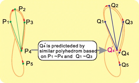
Illustration of topologically equivalent attractors and topologically equivalent position. The two attractors M _X and M _Y are reconstructed from the original system by lagged-coordinates of its components X and Y. These two reconstructed attractors are topological equivalent. There are two short time-series {P _i} and {Q _i}(i = 1, 2, ⋯) on these two topologically equivalent attractors, respectively. And we call two points as topologically equivalent position, taking P ₄ and Q ₄ for example, if and only if the relative distance from P ₄ and Q ₄ to any other points on their corresponding attractors are invariant

where γ is a constant.

We also assume that the relative position of points P _i, Q _i(i = 1, 2, ⋯) on the reconstructed attractors M _X, M _Y are known. Next, we use the information defined in (2) to detect causal relation between these two time-series from the topologically equivalent attractors.

In order to identify the causality between two time-series from their topologically equivalent attractors, first we use the information of P ₁ ∼ P _i and Q ₁ ∼ Q _i − 1 to predict $Q_i^{\prime }$. For example, we use P ₁ ∼ P ₄ and Q ₁ ∼ Q ₃, to predict $Q_4^{\prime }$,where $Q_4^{\prime }$ is decided by similar polyhedron based on P ₁ ∼ P ₄ and Q ₁ ∼ Q ₃ by using (2) . The next important step is to evaluate this prediction. Our criterion is to check the error between the predicted point $Q_4^{\prime }$ and the real point Q ₄. We denote the error as

$$ϵ=\left|Q_4^{\prime }-Q_4\right|.$$ 3

If the error ϵ is sufficiently small (less than 10⁻³), it implies an accurate prediction from P ₄ to Q ₄. In the same way, we can check other points until all the points are evaluated. Finally, we obtain the mean error or the total error. If they are sufficiently small, it means that the information of {P _i}, (i = 1, 2, ⋯) can predict {Q _i}, (i = 1, 2, ⋯). This also implies that {P _i}, (i = 1, 2, ⋯) has strong relationship with {Q _i}, (i = 1, 2, ⋯). In other words, the error can reflect the causal relation between these two variables X and Y. Clearly, even three points are sufficient to estimate the TEP between two time-series in theoretically (to produce ‘two distances’ needs three points at least), which is a major advantages of this method.

However, to directly evaluate the error ϵ of Eq. (3) is not a trivial problem. In particular, for a high dimensional system, it is very difficult to calculate the predicted point Q _4i because we need to solve a large number of nonlinear equations. Here, instead of the error ϵ of Eq. (3), we evaluate the following relative error.

$${\epsilon }_{\mathit{ij}}=\frac{\left|r_{\mathit{ij}}/r_{12}-D_{\mathit{ij}}/D_{12}\right|}{D_{\mathit{ij}}/D_{12}},i\ge 3,i>j,j=1,2,\cdots ,$$ 4

where r _ij is the distance from the predicted points to the real data points. Next, we show that it is not necessary to calculate the predicted points for the error evaluation. From Fig. 2, we know r ₁₂ = d ₁₂ . Therefore, ε _ij can rewritten as

$${\epsilon }_{\mathit{ij}}=\frac{\left|r_{\mathit{ij}}-\gamma D_{\mathit{ij}}\right|}{\gamma D_{\mathit{ij}}},$$ 5

Clearly, we substitute Q _i into (5), i.e., substitute d _ij into (5), then the error ε _ij can be obtained without solving $Q_i^{\prime }$. Since d _ij and D _ij is known, it is easy and straightforward to calculate the relative error ε _ij . Therefore, small error ε _ij implies that the predicted $Q_i^{\prime }$ is in the near neighbor of Q _i or is accurate.

We further scale the error ε _ij by the exponential function so that the error is normalized between 0 and 1. Therefore, the final score of a pair of observed time-series is defined as:

$$\epsilon =\frac{1}{n-1}{\sum }_{i=3}^n\left(\frac{1}{i-1}{\sum }_{j=1}^{i-1}\frac{1}{\mathit{exp}\left({\epsilon }_{\mathit{ij}}\right)},i\ge 3,i>j,j=1,2,\dots ,\right)$$ 6

where n is the number of the time points (samples) for error estimation. Generally, we use leave-one-out scheme to evaluate all the observed time points (samples).

By using this score function, we identify the causal relation both for numerical examples and real gene expression data in next two sections.

Remark: Both the CMS method used in [14] and TEP method proposed here used the delay embedding theory for a nonlinear dynamical system but their idea is different. On one hand, the key point of CMS method is to construct ‘Smoothness Map’. The key idea of our TEP method is to obtain barycentric coordinates by tessellation. On the other hand, the CMS method used nerual network to train the data to show whether the cross map can map the nearest neighbors to mutual neighbors. So that it can be used to detect causality (see Fig. 1a-b in [14]). Our TEP method use the relative distances to predict the next time point and then calculate the error between the predicted point and real point (see Fig. 2). By using this to detect the causal relation between two time series or small samples.

Results

To validate the effectiveness of our TEP method, we first apply our TEP method to both several benchmark examples and gene expression data. The theoretical models used here were the same ones used in [6].

Causal relation of logistic difference equations

The first example is logistic difference equations. Since we know the underlying relations between the variables in advance, we just use these mathematical models to identify the validity of our proposed method. Considering the following two coupled Logistic difference equations which exhibit chaotic behavior [23]

$$\left\{\begin{array}{c}X\left(t+1\right)=X\left(t\right)\left[r_x-r_{x}X\left(t\right)-{\beta }_{x,y}Y\left(t\right)\right],\\ Y\left(t+1\right)=Y\left(t\right)\left[r_y-r_{y}Y\left(t\right)-{\beta }_{y,x}X\left(t\right)\right].\end{array}\right.$$ 7

with r _x = 3.8, r _y = 3.5, β _{x, y} = 0.02, β _{y, x} = 0.1, and the initial conditions X(1) = 0.4, Y (1) = 0.2.

By using the TEP method, we first check the bidirectional causal relation and then the unidirectional causal relation of the above system (7) between the variables X and Y. Since the two cases β _{y, x} = 0 or β _{x, y} = 0 are equivalent, without loss of generality, here we consider the case β _{y, x} = 0. The system (7) becomes

$$\left\{\begin{array}{c}X\left(t+1\right)=X\left(t\right)\left[r_x-r_{x}X\left(t\right)-{\beta }_{x,y}Y\left(t\right)\right],\\ Y\left(t+1\right)=Y\left(t\right)\left[r_y-r_{y}Y\left(t\right)\right].\end{array}\right.$$ 8

with the same parameters r _x = 3.8, r _y = 3.5, β _{x, y} = 0.02, and the initial conditions X(1) = 0.4, Y (1) = 0.2. We give the calculation results by using our method shown in Fig. 3a.

Fig. 3.

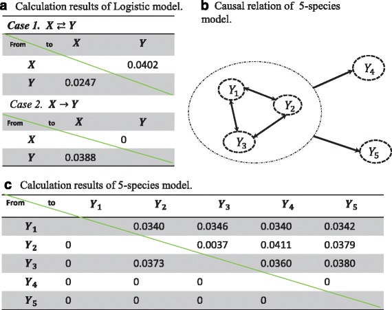
The results of the numerical examples by our method. a. The results of Logistic model by our method (rows → columns). b. The real interaction of a 5-species model. In this model, Y ₁, Y ₂ and Y ₃ are coupled each other, and also Y ₁, Y ₂ , Y ₃ drive Y ₄ and Y ₅ . However, Y ₄ and Y ₅ do not have any effect on Y ₁, Y ₂ and Y ₃ . c. The results of the five species model by our method (rows → columns). Here 0 means that there is no causal relation

Comparing the results in Fig. 3a with those in (7) and (8), clearly our method can identify the causal relation of the two dimensional difference Logistic model correctly. And also comparing with the results in [6], we use much less time points (actually only 10 time points) to identify the causal relation of the logistic model.

Causal relation of 5-species mathematical model

To further verify the effectiveness of our TEP method, we detect the causal relation between the variables of a 5-species model. The model can be described by the following system shown in Fig. 3b.

$$\left\{\begin{array}{c}{Y}_1\left(t+1\right)=Y_1\left(t\right)\left[4-4Y_1\left(t\right)-2Y_2\left(t\right)-0.4Y_3\left(t\right)\right],\\ Y_2\left(t+1\right)=Y_2\left(t\right)\left[3.1-0.3Y_1\left(t\right)-3.1Y_2\left(t\right)-0.93Y_3\left(t\right)\right],\\ Y_3\left(t+1\right)=Y_3\left(t\right)\left[2.12+0.636Y_1\left(t\right)+0.636Y_2\left(t\right)-2.12Y_3\left(t\right)\right],\\ Y_4\left(t+1\right)=Y_4\left(t\right)\left[3.8-0.111Y_1\left(t\right)-0.011Y_2\left(t\right)+0.131Y_3\left(t\right)-3.8Y_4\left(t\right)\right],\\ Y_5\left(t+1\right)=Y_5\left(t\right)\left[4.1-0.082Y_1\left(t\right)-0.111Y_2\left(t\right)-0.125Y_3\left(t\right)-4.1Y_5\left(t\right)\right].\end{array}\right.$$ 9

From Fig. 3b, it is clear that Y ₁, Y ₂ and Y ₃ are coupled each other, and also Y ₁, Y ₂, Y ₃ drive Y ₄ and Y ₅. However, Y ₄ and Y ₅ do not have any effect on Y ₁, Y ₂ and Y ₃. It agrees with our calculation results (by using 15 time points) listed in Fig. 3c.

Both these two simple models show that our method works well by using a small number of samples, i.e., it can detect the causality between the variables correctly.

E. coli Gene expression data

In this section, we apply our method to detect the causal gene regulation between a pair of genes. The gene regulatory network used here is the bacterium E.Coli, as described in [24]. It has been shown that 100 genes can approximate significantly well the statistical properties of the whole network [13, 25]. In order to make comparison, here we also analyze a subnetwork with 100 genes where every gene represents a node and the dynamics of each node (gene) is described by Michaelis-Menten and Hill kinetics. We should point out that for more genes which means the dimensional is much more higher, it still can be disposed by our method. The only thing is that it needs much more time to calculate the errors. Moreover, gene expression data with 10 time points are measured as the same used in [13, 25].

By using the algorithm above, we first calculate ε for each pair of genes. Therefore, there are totally $P_{100}^2,$ i. e. , 9900 εs. We also use the receiver operating characteristics (ROC) curves with different noise level, i.e., noise free, noise level 0.1 and 0.2, respectively. At the same time we also compare our method with the IOTA method used in [13]. The comparing results are shown in Fig. 4. In addition, to evaluate and rank the overall performance, we provide the area under ROC curves (AUC), and the results are shown in Table 1.

Fig. 4.

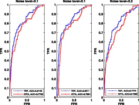
ROC curves of the E. coli network with 100 genes with different noise levels. IOTA represents the method used in [13], and TEP is our method used in this paper

Table 1.

Summary of AUC for E. coli networks

Noise level	AUC for TEP	AUC for IOTA
0	0.8149	0.7732
0.1	0.8211	0.7681
0.2	0.7774	0.7386

From the ROC curves above and the statistic analysis of ROC curves, clearly, TEP is effective to detect the causality of gene regulations for the observed or obtained short time-series data. Comparison results between our method and IOTA method (see Fig. 4) also demonstrate the superiority of TEP on the accuracy.

Yeast gene expression data

Now we detect the causal gene regulations from yeast gene expression data with 10 time points. The network structures were downloaded from the reference [26, 27]. Just like the E.coli gene expression data, here we first conduct the statistics analysis of ROC curves. At the same time, we compare our method with the IOTA method. The results are shown in Fig. 5 and Table 2, which validated the effectiveness of our method.

Fig. 5.

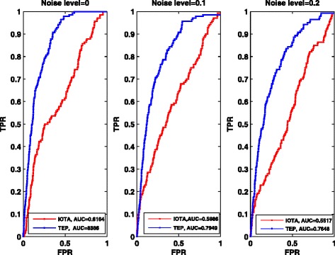
ROC curves of the Yeast network with 100 genes with different noise levels. IOTA represents the method used in [13], and TEP is our method used in this paper

Table 2.

Summary of AUC for yeast networks

Noise level	AUC for TEP	AUC for IOTA
0	0.8386	0.6164
0.1	0.7949	0.5986
0.2	0.7648	0.5517

Rat circadian rhythm gene expression data

Circadian rhythm is fundamentally important for mammals in their physiological processes. To identify the important circadian genes and their roles in their relevant processes is important to elucidate their mechanism of rhythms, in particular, at a network level. In fact, there exists many key circadian genes and functional organization interaction, which generate circadian oscillations. Based on the rat circadian rhythm gene expression data [28], we detect the causal relations among genes by our method.

For circadian rhythm related genes [29, 30], there are 18 key circadian genes identified in mammals and also extensively studied. We further add 22 circadian related genes which all have protein interactions and phosphorylations relationships with the 18 key circadian genes. In other words, we mainly study the causal relations among 40 genes by using the gene expression data. The detail function relationship can be found in [28] (Fig. 2 in [28]). Figure 6 and Table 3 show the ROC curves and the AUC as well as the comparison result, which are obtained based on the gene expression data with 18 time points as the same case in [28].

Fig. 6.

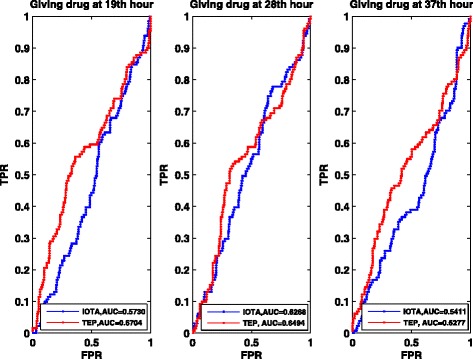
ROC curves of the Rat circadian rhythm with 18 key related genes by applying drug at different time points. IOTA represents the method used in [13], and TEP is our method used in this paper

Table 3.

Summary of AUC for circadian rhythm networks

Time points of using drug	AUC for TEP	AUC for IOTA
19th hour	0.6704	0.5730
28th hour	0.6494	0.6268
37th hour	0.6277	0.5411

In order to make our results more clearly, we give the real gene regulatory network of 100 genes of E. coli and Yeast in Figs. 7 and 8. The results of the above three gene expression data show that TEP method works well even with a small number of samples. Comparing with the IOTA method, the truth positive rate (TPR) are higher with the same false positive rate (FPR), which means that our method is effective to detect the causal relation than IOTA method.

Fig. 7.

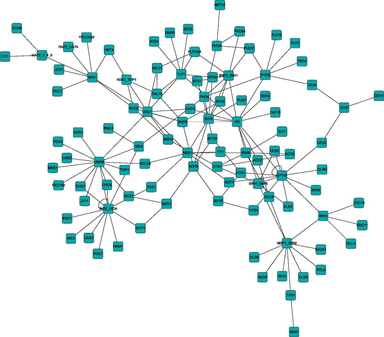
The real gene regulatory network of E.Coli with 100 genes

Fig. 8.

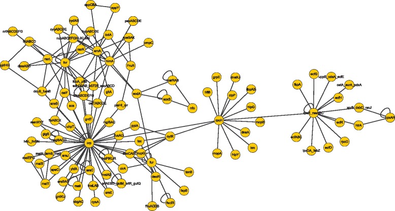
The real gene regulatory network of Yeast with 100 genes

Discussion

How to detect the causal relations from short time-series data is really very important. Especially for the genes, because the obtained causal relations among the genes can provide valuable information and insights into topological structures of gene regulatory networks. Besides the gene regulatory networks, our method can be used in many other complex networks. However, we must also point out that there still exist false predictions, e.g., many false prediction by the circadian rhythm gene expression data. As a future topic, we will study the dependence of our method on the data and its length.

Conclusion

In this work, a new method which called topologically equivalent position method is proposed. It is a prediction-based method. It can be effectively used to detect the causality of the observed short time-series data or very small samples. Both the numerical examples and gene expression data have been used to validate the proposed method. Different from the existed method, such as Granger causality and CCM, our method not only is simple in terms of computational procedure, but also can be applied to nonlinear systems. The most important is that it can identify the causality for the observed observed time-series just from short time points. This is very useful for real-world data, in particular, the gene expression data, which are typically very short (≈10 points).

Authors’ contributions

Conceived the study: BZ, WL, LC. Did simulation: YS, XL. Wrote the paper:BZ, WL, YS, XL, LC. All authors read and approved the final manuscript.

Ethics approval and consent to participate

All participants gave written informed consent for participation in their respective studies and the conduct of genetic research, and the studies in which the subjects were enrolled were approved by their respective institutional review boards.

Consent for publication

Not applicable.

Competing interests

The authors declare that they have no competing interests.

Publisher’s Note

Springer Nature remains neutral with regard to jurisdictional claims in published maps and institutional affiliations.

References

- 1.Schiff SJ, So P, Chang T, Burke RE, Sauer T. Detecting dynamical interdependence and generalized synchrony through mutual prediction in a neural ensemble. Phys Rev E. 1996;54:6708–6724. doi: 10.1103/PhysRevE.54.6708. [DOI] [PubMed] [Google Scholar]
- 2.Arnhold J, Grassberger P, Lehnertz K, Elger CEA. Robust method for detecting interdependences: application to intracranially recorded EEG. Physica D. 1999;134:419–430. doi: 10.1016/S0167-2789(99)00140-2. [DOI] [Google Scholar]
- 3.Rosenblum M, Pikovsky A. Detecting direction of coupling in interacting oscillators. Phys. Rev. E. 2001;64:045202(R). doi: 10.1103/PhysRevE.64.045202. [DOI] [PubMed] [Google Scholar]
- 4.Schreiber T. Measuring information transfer. Phys Rev Lett. 2000;85:461–464. doi: 10.1103/PhysRevLett.85.461. [DOI] [PubMed] [Google Scholar]
- 5.Hirata Y, Aihara K. Identifying hidden common causes from bivariate time-series: a method using recurrence plots. Phys Rev E. 2010;81:016203. doi: 10.1103/PhysRevE.81.016203. [DOI] [PubMed] [Google Scholar]
- 6.Sugihara G, May R, Ye H, Hsieh C, Deyle E, Fogarty M, Munch S. Detecting causality in complex ecosystems. Science. 2012;338:496–500. doi: 10.1126/science.1227079. [DOI] [PubMed] [Google Scholar]
- 7.Granger CWJ. Investigating causal relations by econometric models and cross-spectral methods. Econometrica. 1969;37:424–438. doi: 10.2307/1912791. [DOI] [Google Scholar]
- 8.Engle RF, Granger CWJ. Co-integration and error correction: representation, estimation, and testing. Econometrica. 1987;55:251–276. doi: 10.2307/1913236. [DOI] [Google Scholar]
- 9.Hiemstra C, Jones JD. Testing for linear and nonlinear granger causality in the stock price-volume relation. J. Finance. 1994;49:1639–1664. [Google Scholar]
- 10.Faes L, Nollo G, Porta A. Information-based detection of nonlinear granger causality in multivariate processes via a nonuniform embedding technique. Phys Rev E. 2011;83:051112. doi: 10.1103/PhysRevE.83.051112. [DOI] [PubMed] [Google Scholar]
- 11.Ding M, Chen Y, Bressler SL. Handbook of time-series analysis. Weinheim, Germany: Wiley-VCH; 2006. pp. 437–460. [Google Scholar]
- 12.Dhamala M, Rangarajan G, Ding M. Estimating granger causality from Fourier and wavelet transforms of time-series data. Phys Rev Lett. 2008;100:018701. doi: 10.1103/PhysRevLett.100.018701. [DOI] [PubMed] [Google Scholar]
- 13.Hempel S, Koseska A, Kurths J, Nikoloski Z. Inner composition alignment for inferring directed networks from short time-series. Phys Rev Lett. 2011;107:054101. doi: 10.1103/PhysRevLett.107.054101. [DOI] [PubMed] [Google Scholar]
- 14.Ma H, Aihara K, Chen L. Detecting causality from nonlinear dynamics with short-term time series. Sci Rep. 2014;4:7464. doi: 10.1038/srep07464. [DOI] [PMC free article] [PubMed] [Google Scholar]
- 15.Runge J, Heitzig J, Petoukhov V, Kurths J. Escaping the curse of dimensionality in estimating multivariate transfer entropy. Phys Rev Lett. 2012;108:258701. doi: 10.1103/PhysRevLett.108.258701. [DOI] [PubMed] [Google Scholar]
- 16.Runge J, Heitzig J, Marwan N, Kurths J. Quantifying causal coupling strength: a lag-specific measure for multivariate time-series related to transfer entropy. Phys Rev E. 2012;86:061121. doi: 10.1103/PhysRevE.86.061121. [DOI] [PubMed] [Google Scholar]
- 17.Takens F. Detecing strange attractors in turbulence, lecture notes in mathematics Vol. 898, edited by D. A. Rand and L. S. Young. Berlin: Springer; 1981. p. 366. [Google Scholar]
- 18.Sauer T, Yorke JA, Casdagli M. Embedology. J Stat Phys. 1991;65:579–616. doi: 10.1007/BF01053745. [DOI] [Google Scholar]
- 19.Stark J. Delay embeddings for forced systems I. Deterministic forcing. J. Nonlinear Sci. 1999;9:255–332. doi: 10.1007/s003329900072. [DOI] [Google Scholar]
- 20.Stark J, Broomhead DS, Davies ME, Huke J. Delay Embeddings for forced systems. II. Stochastic forcing. J Nonlinear Sci. 2003;13:519–577. doi: 10.1007/s00332-003-0534-4. [DOI] [Google Scholar]
- 21.Mees A. Int. dynamics systems and tesselations: detecting determinism in data. J. Bifurcation. Chaos. 1991;1:777–794. [Google Scholar]
- 22.Hirata Y, Shiro M, Takahashi N, Aihara K, Suzuki H, Mas P. Approximating high-dimensional dynamics by barycentric coordinates with linear programming. Chaos. 2015;25:013114. doi: 10.1063/1.4906746. [DOI] [PubMed] [Google Scholar]
- 23.Lloyd AL. The coupled logistic map: a simple model for the effects of spatial heterogeneity on population dynamics. J Theor Biol. 1995;173:217–230. doi: 10.1006/jtbi.1995.0058. [DOI] [Google Scholar]
- 24.Shen-Orr SS, Milo R, Mangan S, Alon U. Network motifs in the transcriptional regulation network of Escherichia Coli. Nat Genet. 2002;31:64–68. doi: 10.1038/ng881. [DOI] [PubMed] [Google Scholar]
- 25.Bulcke TV, Leemput KV, Naudts B, et al. SynTReN: a generator of synthetic gene expression data for design and analysis of structure learning algorithms. BMC Bioinformatics. 2006;7:43. doi: 10.1186/1471-2105-7-43. [DOI] [PMC free article] [PubMed] [Google Scholar]
- 26.Van den Bulcke T, Van Leemput K, Naudts B, van Remortel P, Ma H, Verschoren A, De Moor B, Marchal K. SynTRen generator, version 1.1.3. 2006. http://homes.esat.kuleuven.be. [DOI] [PMC free article] [PubMed]
- 27.Guelzim N, Bottani S, Bourgine P, Kepes F. Topological and causal structure of yeast transcriptional regulatory network. Nat Genet. 2002;31:60–63. doi: 10.1038/ng873. [DOI] [PubMed] [Google Scholar]
- 28.Wang Y, Zhang XS, Chen LA. Network biology study on circadian rhythm by integrating various OMICS data. OMICS: a journal of. Integr Biol. 2009;13:313–324. doi: 10.1089/omi.2009.0040. [DOI] [PubMed] [Google Scholar]
- 29.Ueda HR, Hayashi S, Chen W, Sano M, Machida M, Shigeyoshi Y, et al. System-level identification of transcriptional circuits underlying mammalian circadian clocks. Nat Genet. 2005;37:187–192. doi: 10.1038/ng1504. [DOI] [PubMed] [Google Scholar]
- 30.Ko CH, Takahashi JS. Molecular components of the mammalian circadian clock. Hum Mol Genet. 2006;15:R271. doi: 10.1093/hmg/ddl207. [DOI] [PubMed] [Google Scholar]
Associated Data
This section collects any data citations, data availability statements, or supplementary materials included in this article.
Data Availability Statement