A Framework for Modeling the Relationship Between Cellular Steady-state and Stimulus-responsiveness

Abstract

In cell signaling systems, the abundances of signaling molecules are generally thought to determine the response to stimulation. However, the kinetics of molecular processes, for example receptor trafficking and protein turnover, may also play an important role. Few studies have systematically examined this relationship between the resting state and stimulus-responsiveness. Fewer still have investigated the relative contribution of steady-state concentrations and reaction kinetics. Here we describe a mathematical framework for modeling the resting state of signaling systems. Among other things, this framework allows steady-state concentration measurements to be used in parameterizing kinetic models, and enables comprehensive characterization of the relationship between the resting state and the cellular response to stimulation.

I. Introduction

Cell systems respond to external stimuli through a coordinated network of biochemical reactions mediated by any number of molecular species. Although it is customary to think of these systems as being “at rest” prior to stimulation, a growing number of studies have demonstrated that the resting state of a cell prior to stimulation can be a powerful determinant of the response. For example, with regards to stimulation by the death-inducing TNF superfamily member TRAIL, studies have shown that cells may be sensitized via up-regulation of the TRAIL receptor DR5 (Dolloff et al., 2011) or caspase 8 (Fulda et al., 2001), down-regulation of TRADD (Kim et al., 2011) or c-FILP (Li et al., 2011), or alternatively desensitized by up-regulation of Bcl-XL (Hinz et al., 2000) or Bcl-2 (Fulda et al., 2002) (reviewed in Zhang and Fang, 2005).

By contrast, in other systems it has been shown that the kinetics of species turnover – not their outright abundance – determine the response to stimulation. For example, high turnover of the Epo receptor is required to maintain a linear, non-refractory response over a broad range of Epo concentrations (Becker et al., 2010), while high turnover of the inhibitor of NFκB is required to distinguish acute inflammatory stimuli from metabolic stress conditions (O’Dea et al., 2008). Studies like these highlight an important dichotomy in the resting state of a cell. In one hand are the concentrations of molecules prior to stimulation, and in the other are the rates of the biochemical processes in which they participate. How do each of these facets of the resting state affect the cellular response to stimulation?

Because systematic changes in the resting states of living cells are difficult to engineer, investigating this relationship cannot be addressed by laboratory science alone. For example, short interfering (si) RNA can be used to reduce the concentration of a specific gene product, but this reduction is effected by interfering with the translation of the product (Fire et al., 1998; Izant and Weintraub, 1984). Changes in stimulus-responsiveness due to siRNA knockdown may, therefore, be caused by a reduction in the concentration of the target species, reduction in the kinetics of its turnover, or both. Furthermore, RNA dilution in rapidly dividing cells (Bartlett and Davis, 2006) or secondary induction of the mammalian interferon response (Reynolds et al., 2006) may further cloud interpretation of the results.

Using a mathematical model, the behavior of a system can be studied rapidly and in isolation, providing a sort of sufficiency test for proposed mechanisms of cellular responsiveness (Faller et al., 2003; Kearns and Hoffmann, 2009; and Kitano, 2002). The steady-state of a model, discussed in further detail below, is furthermore a good approximation for the resting state of the system. A complication that arises in models when trying to characterize the relationship between steady-state and stimulus-responsiveness, however, is that models of cell systems are typically nonlinear. As such, the steady-state must often be found numerically, and this compromises the modeler’s ability to investigate its role in stimulus-responsiveness.

To that end, in this chapter we describe a method for deriving an analytical expression for the steady-state of a common class of models, called mass action models. From this analytical expression, we go on to give precise steps for introducing systematic changes to the steady-state concentrations of molecular species and the rates of biochemical processes in which they participate. In doing so, we demonstrate how specific hypotheses can be generated about the resting state of a system and its impact on stimulus-responsiveness. Examples include:

• Are my measurements of steady-state concentrations and kinetic rate constants consistent with the proposed model?

• Is a change in the steady-state concentration or activity of a particular species sufficient to explain the changes I observed in the system’s response to stimulation?

• Can I expect a system at a particular resting state to exhibit a certain response to stimulation?

The remainder of this text is divided into the following sections: “Overview of Algorithm,” in which we provide a verbal description of the steps required to model a system and derive a solution to its steady-state; “Biological Insights,” in which we demonstrate how a model at steady-state can help generate hypotheses about the relationship between the resting state of a system and its response to stimulation; “Open Challenges,” in which we describe limitations of the method and potential avenues for refinement; “Computational Methods,” in which we provide step-by-step instructions for modeling a system and manipulating its steady-state; and finally “Further Reading,” where we offer some references for further reading on the subject of modeling, steady-state, and parameterization, and dynamic response analysis.

II. Overview of Algorithm

For the purposes of this manuscript we assume that the system to be studied can be described by a biochemical reaction network (BRN). A BRN consists a set of a set of molecular species and a set of biochemical reactions. The set of species must contain every species consumed or produced by the reactions. Neither every species nor every reaction need be elementary – a species may refer to a complex biomolecule like a ribosome, for example, and a reaction to a multistep process like protein synthesis.

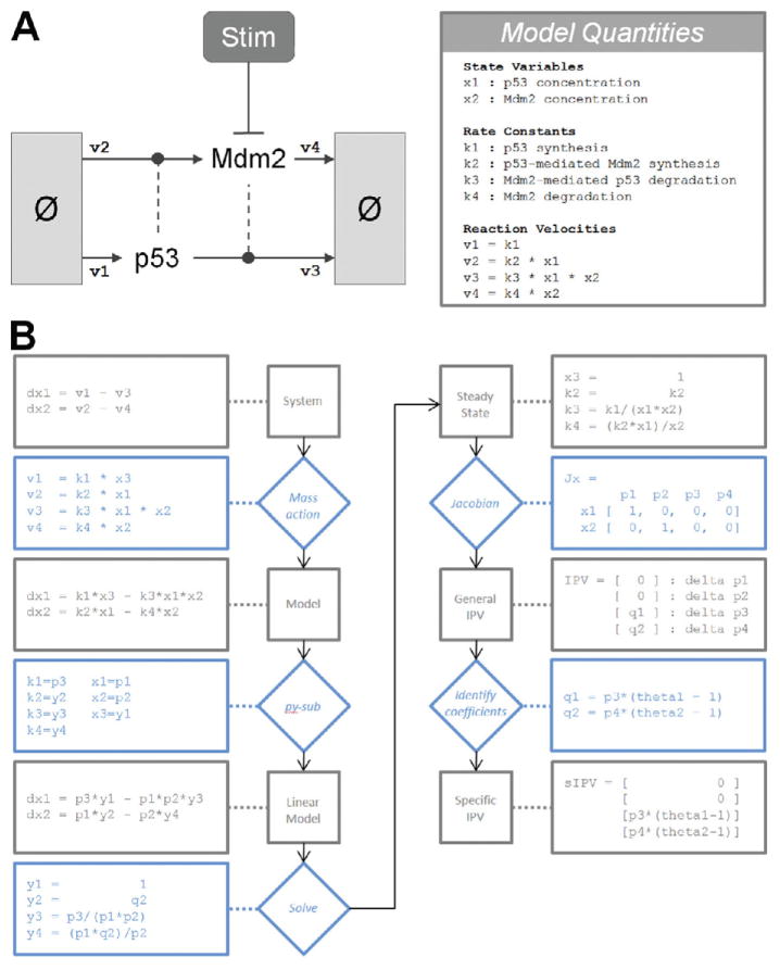
A simple BRN to illustrate the steps used in the forthcoming algorithm is the activation of the tumor suppressor p53. This network consists of two species, p53 and Mdm2, and four reactions. These reactions describe the process by which p53 and Mdm2 self-regulate through coordinated synthesis and degradation. Specifically, p53 is constitutively synthesized but degraded in an Mdm2-dependent manner. Mdm2 is synthesized in a p53-dependent manner but constitutively degraded. An illustration of this network is given in Fig. 1, as are all steps used in the forthcoming algorithm.

Fig. 1.

Schematic of the simple model of p53 activation and regulation by Mdm2 used throughout this document. Below that, a flowchart of a mathematical framework for modeling the resting state. Diamonds represent major steps in the framework while boxes represent the outcome of those steps. The outside track illustrates the results of this framework when applied to the p53 model. (For color version of this figure, the reader is referred to the web version of this book.)

A. Model the System of Interest Using Mass Action Kinetics

We further assume that the BRN used to describe our system can be modeled using mass action kinetics. Mass action assumes that the velocity of a chemical reaction – or the rate at which it converts reactants into products – is proportional to the product of each reactant raised to some power. This power is often equal to the stoichiometry of the reactant and is, therefore, simply one. Note too that when we refer to a species of a mass action model, we nearly always mean the abundance of that species. The resultant mathematical expression for the velocity of the reaction is often called a rate equation.

There are four reactions in the p53 model, which cumulatively describe the synthesis and degradation of p53 and Mdm2. Under mass action, the velocity of, say, p53 degradation is proportional to the product of p53 and Mdm2. Equivalently, we can say that the velocity of p53 degradation is equal to the product of p53, Mdm2, and a proportionality constant. This proportionality constant is commonly called a rate constant.

Once rate equations have been written for each chemical reaction, we apply the principle of mass balance to arrive at a set of governing equations that describes how every species behaves over time. This principle holds that the rate at which a species changes over time is equal to the sum of reaction velocities for which that species is produced, minus the sum of reaction velocities for which it is consumed. For example, p53 is produced by a zero-order synthesis reaction and consumed by a second-order degradation reaction. Consequently, we can write that the first derivative of p53 with respect to time is equal to the velocity of synthesis minus the velocity of degradation. In this way, application of mass action kinetics to any BRN yields a system of ordinary differential equations that describes the instantaneous rate of change for every species as a function of the reaction velocities.

Mass action may not always be appropriate to model the behavior of a BRN. A key assumption of the rate equation is that of spatial homogeneity. That is, there are no gradients in the concentration of any species and the local concentration at any point in space is equal to the global concentration (Grima and Schnell, 2008). This condition is violated when there are differences in the diffusivity of the species, due to either complex formation, tethering to subcellular structures, or compartmentalization (Kholodenko, 2009). Such systems are more appropriately modeled using reaction diffusion equations, reviewed in Slepchenko et al., 2002. A second assumption of the rate equation is that the concentration of each participating species is sufficiently “large” (Sreenath et al., 2008). If this is not the case, then random fluctuations can no longer be ignored and the reaction velocity must be modeled by a propensity function, called the chemical master equation (Gillespie, 1992). Extending the method presented here to systems where the assumptions of mass action fail is the subject of future research, and is discussed in Open Challenges.

B. Derive an Expression for the Steady-state of the Mass Action Model

For any mass action model there exists at least one set of reaction velocities where every species is being produced as quickly as it is being consumed. When this is the case, the model is said to be at steady-state. In this chapter, we equate steady-state with the resting state, but remark that a more sophisticated relationship between the two could be the subject of future work.

Every mass action model will have one or more trivial steady-states. These are steady-states in which all reaction velocities are zero. Closed systems, or systems that don’t consider synthesis and degradation, always have a trivial steady-state in which every species’ abundance is zero. Open systems also require that one or more synthesis rate be zero. An example of a trivial steady-state in the p53 model is one where there is neither p53 nor synthesis thereof. Since trivial steady-states are of little physiological interest, how might we identify nontrivial steady-states. More pointedly, in order to examine the relationship between steady-state and the dynamic response, how might all nontrivial steady-states be identified?

Mathematically, finding steady-states is equivalent to solving the system of equations that results when we set the rate of change of every species equal to zero. If the system happens to be linear in the variables of interest, then a solution can often be found quite easily. The key then is simply to find a subset of species and rate constants that may be treated as variables such that the resulting system of equations is linear. Ideally, the complement of that subset will be species and rate constants for which accurate measurements are available, since these are elements for which numerical values will need to be given prior to simulation. A detailed description of this process, which we call py-substitution, is given below.

1. Develop and Apply a py-substitution Strategy

From the set of all rate constants and species abundances, identify a substitution strategy by which elements with known values are replaced by a p and elements with unknown values are replaced by a y. We refer to these quantities as parameters and variables, respectively. Every substitution strategy must also satisfy the following conditions: (1) the resultant system of equations is linear in y, and (2) there are at least as many variables as there are linearly independent equations. The latter of these ensures that the py-substituted system of equations is not overdetermined.

Zero-order reaction velocities and velocities with exponents not equal to unity introduce a further complication: the former cannot be substituted by parameters nor the latter by variables. To do so violates the linearity constraint. If this constraint is undesirable, a work-around is to introduce a pseudospecies. For example, the velocity of p53 synthesis in our p53 model is independent of any species abundance. That is, the rate of synthesis is constant and equal to a single rate constant. If a reliable measurement exists for that rate constant, we may wish to substitute it with a parameter rather than a variable. But because doing so would violate the linearity requirement, we let the velocity be equal to the product of a first order rate constant and a pseudospecies. The latter of these we substitute normally with a variable and, once the system of steady-state equations has been solved, go back and make sure its value is unity.

A similar tactic can be used for reaction velocities that are superlinear in one of their reactants. If no reliable estimate exists for the abundance of the reactant, we may wish to substitute it with a variable rather than a parameter. Since doing so results in a superlinearity in y, we replace the reactant with a pseudospecies whose exponent is unity. The pseudospecies can then be substituted normally with a variable. After solving the system of steady-state equations, we go back and ensure that the steady-state expressions for the pseudospecies and the superlinear reactant are equal.

2. Solve the Linear System

After developing a py-substitution strategy, the system of steady-state equations is rendered linear in the variables. This allows us to rewrite the system using matrix notation. Specifically, we can write that the product formed by a matrix of parameters C with a column vector of variables y equals a column vector of zeros. We call this matrix of parameters the coefficient matrix:

$$\mathit{Cy}=\mathit{0}$$ (1)

The solution to this equation is precisely the null space of the coefficient matrix. Most modern mathematics software can derive a symbolic basis for the null space, so long as the matrix is not too large. If it is large (say, over 100 rows and columns, approximately equivalent to a system containing 100 species and reactions), then so too is the number of row operations needed to derive a basis. Since the elements in the matrix are symbolic, they can seldom can be reduced after each row operation. As a result, certain elements will grow geometrically in complexity and consume all the available RAM on the host device, causing a de facto arrest of the computation. Not all software packages handle this explosion equally well. In our experience, Maple outperforms both Mathematica and Matlab.

What is the benefit of a symbolic solution to the steady-state equation over a numerical one? With the latter, every independent parameter is a numeric value, which by the coefficient matrix is mapped efficiently to a value for each variable such that the system is at steady-state. The downside of this approach is that the contribution of each parameter to the variables is lost during the calculation. If the values of the independent parameters change, as is often required during the analysis of a mass action model, the values for the dependent variables must be calculated anew. With a symbolic solution, the contribution from each parameter to the steady-state expression of each variable is preserved. This has several advantages. (1) The relationship between a variable and an independent parameter can sometimes be identified directly from its steady-state expression. For example, the expression may reveal that a certain concentration scales linearly or nonlinearly with another species’ concentration, or that the concentration does not depend at all on certain reaction rates. (2) More generally, the sensitivity of each dependent variable to each independent parameter can be calculated, so that, for example, changes in parameter values can be identified that only affect a certain subset of variables. This is precisely the approach we use below to selectively alter the steady-state turnover of p53 and Mdm2.

3. Derive a General Expression for the Vector of Variables

A basis for the null space of the coefficient matrix spans the solution to the steady-state equation. If we let the vector of variables be any linear combination of null space basis vectors, then the system will be at steady-state no matter what values we assign to the parameters. By any linear combination, we mean that the coefficient of each basis vector can be any real-valued number. If the basis vectors are arranged as columns in a matrix, this is equivalent to postmultiplying that matrix by a column vector of real-valued coefficients.

4. Resolve Any Constraints Imposed by Pseudospecies

Once a general expression is derived for the vector of variables, we must resolve any additional constraints imposed by the pseudospecies. Typically these will have the form y_a = y_b² in the case of a superlinearity, or y_a = 1 in the case of a sublinearity. The solution to these equations is not always straightforward, especially the former. Whichever mathematics software was employed to derive the null space for the coefficient matrix, however, can be used again here to solve the pseudospecies constraints.

Another complication that may arise during this step is that a superlinear constraint will yield two or more possible solutions. In theory, this presents a very interesting scenario where two or more values for the same species result in an otherwise identical steady-state. In other words, this may represent a bi- or multi-stability. In practice, our experience has been that when two solutions are possible, one of them is always negative and, therefore, physiologically infeasible. Furthermore, bistabilities reported in the literature typically manifest themselves in all of the species, not just one. Therefore, a practical resolution to this complication has been to keep both symbolic solutions but discard the infeasible one after numerical values are given to the parameters.

5. Reverse the py-substitution

Once the steady-state equation is solved and an expression derived for the vector of variables, one may wish to revert the substitution so that the relationships between variables and parameters are expressed in terms of species and rate constants. For simple systems, this can yield insight into how steady-state is achieved. For larger systems, these relationships can become intractable. Furthermore, for subsequent steps in this algorithm, the parametric description of steady-state can be the more useful of the two. For these reasons, reverting the py-substitution is an optional step.

If reversion is desired, note that a technical complication was introduced by the linear combination of null space basis vectors. Specifically, the forward py-substitution results in a linear system that is solvable but underdetermined. If this was not the case then the coefficient matrix would not have a null space. By taking a linear combination of the basis vectors, we effectively identify dimensions of the null space that are independent and thus need to be given a numerical value. In other words, the original py-substitution contained too many variables. A number of these variables equal to the dimension of the null space must become parameters. Fortunately, by scaling the basis vectors such that they are normalized with respect to the desired variable, we have a fair amount of freedom in specifying which variables are to become parameters.

Once this is done, we are left with an equation where the left hand side is the original vector of variables, and the right hand side is the product of the matrix of null space basis vectors and the vector of coefficients. Letting these elements be represented by y, N, and q, respectively, the equation looks like the following.

$$\mathit{y}=\mathit{Nq}$$ (2)

It is precisely this equation that preserves the steady-state in our mass action model. The left hand side is within the domain of the inverse of the original py-substitution and can be reverted quite easily. The right hand side is a function of parameters and basis vector coefficients. The latter of these is not within the domain of the inverse py-substitution, so we must first convert these to variables. Fortunately, this conversion can be easily identified from the equation itself. By the derivation of the null space basis via row reduction of the coefficient matrix, there will exist at least one row in N for which only one column contains a nonzero entry. If the vector is scaled to this entry, then the row defines a one-to-one mapping between basis vector coefficients and variables. This mapping restores the right hand side to the domain of the inverse py-substitution, thus making the full reversion possible.

C. Identify the Isostatic Subspace of the Mass Action Model

Once we have derived an expression for the steady-state of our mass action model, we may wish to characterize the relationship between the dynamics of the system and its rate constants and steady-state abundances. The former of these is not straightforward, however, because changes in kinetic rate constants often result in changes to the abundances. To isolate the effects of changes in rate constants on system dynamics, we must derive an expression for the isostatic subspace of the model, that being the set of all parameter perturbations that do not in turn alter the steady-state species abundances.

1. Calculate the Jacobian Matrix of Partial Sensitivities in Abundances With Respect to Parameters

The first step in deriving the isostatic subspace is to define precisely what we mean by a perturbation in parameters that in turn does not alter the steady-state abundances. From our derivation of the steady-state above, we have that every species abundance is equal to some function of parameters and null space basis vector coefficients. It is convenient at this point to simply consider the latter of these as parameters as well. Some species equate one-to-one with a single parameter; other species are equal to complex expressions in the parameters. Either way, we are interested in a change in parameters Δp that, when added to the original set of parameters p, results in a change in species Δx equal to zero. This is expressed succinctly by the following equation.

$$\mathrm{\Delta }\mathit{p}\in \{\mathrm{\Delta }\mathit{p}\ne 0:\mathrm{\Delta }\mathit{x}=\mathit{x}(\mathit{p})-\mathit{x}(\mathit{p}+\mathrm{\Delta }\mathit{p})=0\}$$ (3)

A valid change in parameters is thus any that satisfies

$$\mathit{x}(\mathit{p})=\mathit{x}(\mathit{p}+\mathrm{\Delta }\mathit{p})$$ (4)

The right hand side of this equation can be approximated by a truncated Taylor series, as follows,

$$\mathrm{\Delta }\mathit{x}(\mathit{p}+\mathrm{\Delta }\mathit{p})\approx \mathit{x}(\mathit{p})+{\mathit{J}}_x\mathrm{\Delta }\mathit{p}$$ (5)

where J_x is the Jacobian matrix whose elements are the partial derivatives of each species with respect to each parameter. The first step in deriving the isostatic subspace is, therefore, to calculate this matrix, which can be done efficiently using our choice of mathematics software.

2. Derive a Basis for the Null Space of the Jacobian Matrix

We are now confronted with the same situation as we were when deriving an expression for the steady-state. Since we want our new vector of species abundances to equal the old one, we require that

$${\mathit{J}}_x\mathrm{\Delta }\mathit{p}=\mathbf{0}$$ (6)

In other words, the change in parameters must reside within the null space of the Jacobian matrix. Equivalently, we call this particular null space the isostatic subspace, since it contains every perturbation in the parameters that does not affect the steady-state species abundances. A basis for this subspace can be derived as before.

3. Derive a General Isostatic Perturbation Vector

Every dimension in the isostatic subspace is a degree of freedom through which we can introduce an isostatic perturbation. A general expression for an isostatic perturbation then is simply the product of a matrix whose columns are the basis vectors of the isostatic subspace and a vector of basis vector coefficients. Notice how closely this step mirrors the derivation for an expression for the vector of variables, above. Once this multiplication is done, we are left with a general isostatic perturbation vector.

4. Derive a Specific Isostatic Perturbation Vector

Each degree of freedom in the general isostatic perturbation vector may introduce a perturbation that, in isolation, is of no physiological interest. For example, in the p53 model, we may be interested in introducing a perturbation that alters the rate of synthesis and degradation of p53. There is no guarantee that this perturbation exists as a single vector in our basis for the isostatic subspace. Therefore, the final step is to identify a specific combination of basis vectors to achieve the desired perturbation. In Section V, below, all of these steps are illustrated in detail as they are applied to our simple model of p53 activation.

III. Biological Insights

In this section, we illustrate some of the insights and hypotheses that can be generated from the steady-state and isostatic subspace of a mass action model. First, we show that statics and kinetics must cooperate to achieve steady-state. If an expression for the steady-state is known, then static parameters can be used to calculate the values for some, but not all, kinetic parameters. The fact that not all kinetic parameters can be calculated is related to the fact that the dynamic response to perturbation cannot be uniquely determined from static information alone. Using our simple model for the activation of the tumor suppressor p53, we show that the kinetics of homeostatic protein turnover determine the dynamic response of p53 to DNA damage.

A. Explicit Derivation of Kinetic Rate Constants From Static Measurements

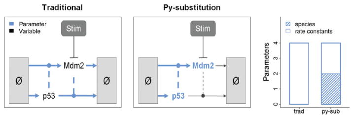
A key motivation for the development of py-substitution was to calculate kinetic rate constants directly from static measurements (Fig. 2). For example, in the p53 model, values can be given for the steady-state abundances of p53 and Mdm2. Just the degradation rates of p53 and Mdm2 are then required to fully parameterize the model. The rates of synthesis can be calculated explicitly using these four parameters and the steady-state expression derived by py-substitution.

Fig. 2.

A comparison of py-substitution versus a traditional parameterization strategy. A traditional strategy requires numeric values for all four rate constants. Using py-substitution, the steady-state abundances of p53 and Mdm2 can be given explicitly. In conjunction with the rates of synthesis of p53 and Mdm2, the degradation rate constants can be calculated such that steady-state is preserved. (For color version of this figure, the reader is referred to the web version of this book.)

By comparison, a traditional parameterization strategy would require that all four kinetic rate constants be specified. The steady-state abundances of p53 and Mdm2 could then be derived numerically by integrating the model to steady-state, but this process is comparatively less efficient. Furthermore, the steady-state behavior of p53 and Mdm2 over a range of synthesis and degradation rates is unknowable except through simulation. If estimates for the steady-state abundances of p53 and Mdm2 exist, then a parameter fitting procedure must be used to infer the optimal values for the kinetic rate constants. This is an example of a “backward problem,” in that the “forward problem” – calculating the steady-state abundances of p53 and Mdm2 given a set of four kinetic rate constants – must be iteratively solved until an optimal set of rate constants is identified. If, however, an expression for the steady-state is known, this backward problem is turned into a forward problem: given the steady-state abundances for p53 and Mdm2 and their rates of degradation, a simple calculation gives the rates of synthesis required to support that steady-state.

The significance of this difference is that making kinetic measurements can be a considerable technical challenge. Typically kinetic parameters must be determined with purified proteins using in vitro assays (Nutiu et al., 2011; Tanious et al., 2008) or must be derived from biochemical assays requiring millions of cells (Schwanhäusser et al., 2011). By contrast, static measurements are often more sensitive and can be performed using fixed cells (Itzkovitz and van Oudenaarden, 2011; Jain et al., 2011). As a result, measuring static variables is easier and more accurate than measuring kinetic ones, and py-substitution allows kinetic rate constants to be derived explicitly from simpler, static measurements.

B. Static Control of the Dynamic Response

Another benefit of py-substitution is that we can systematically evaluate the relationship between dynamic responsiveness and steady-state abundances. This is made possible by the fact that py-substitution allows steady-state abundances to be treated as independent parameters. For example, the dynamic response of p53 to DNA damage is affected by the steady-state abundance of Mdm2. Because we have modeled this abundance as an input parameter, it is straightforward to vary it over a range of values and simulate the p53 response at each value.

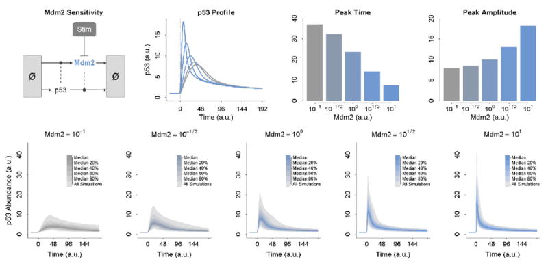
In Fig. 3, we let Mdm2 vary from 0.1 to 10 times its nominal wildtype value. As Mdm2 increases, p53 exhibits a faster and stronger dynamic response. As it decreases, p53 becomes slower and weaker. This is because the rate of p53 degradation scales with the steady-state abundance of Mdm2. As the latter increases, so does the former. Since we have not varied the steady-state abundance of p53 but rather kept it fixed, the rate of p53 synthesis must also scale with the abundance of Mdm2. In other words, a higher steady-state abundance of Mdm2 results in a higher steady-state turnover of p53. The velocity of this turnover partially dictates the dynamics of the p53 response. Homeostatic turnover will be examined in more detail in the next subsection.

Fig. 3.

The effect of the steady-state abundance of Mdm2 on the dynamic response of p53 to stimulation. At top, the steady-state abundance of Mdm2 is varied from 0.1 (light gray) to 10 (dark gray). The result of this variation on the time and amplitude of the p53 response are shown as bar graphs on the right. At bottom, Mdm2 is again varied from 0.1 to 10. Each of the five panels represents a distinct but constant abundance of Mdm2. The abundance of p53 is always 1. The rates of p53 and Mdm2 synthesis and degradation are then allowed to take a random value from a uniform distribution over 0.1 to 10 times their nominal wildtype values. The p53 response to perturbation is simulated for 1000 samples in each panel and the median dynamics plotted. (For color version of this figure, the reader is referred to the web version of this book.)

Interestingly, even though steady-state abundances affect the dynamic response, they do not uniquely determine it. Put another way, the dynamic response to perturbation is underdetermined with respect to the steady-state abundances. This is illustrated in Fig. 3, bottom. Here, each panel depicts the median behavior of 1000 simulations of the p53 model. For a given panel, every simulation has the same steady-state abundance of Mdm2 and p53. The rates of homeostatic turnover of Mdm2 and p53, however, are allowed to take a uniform random value between 0.1 and 10 times their nominal wildtype value. We say that these simulations are isostatic but anisokinetic – their steady-state abundances are identical but their kinetic rate constants are not. This variability in the kinetics causes variability in the dynamics, but is entirely opaque with respect to the steady-state abundances.

C. Kinetic Control of the Dynamic Response

As Fig. 3 shows, isostatic systems can exhibit significant variability in their response to perturbation. This is a consequence of the fact that the steady-state of a mass action model is degenerate with respect to its kinetics; an infinite number of kinetic rate constants can support the same set of steady-state abundances. We call a change in kinetic rate constants that does not affect any steady-state abundances an isostatic perturbation to the parameters, or an isostatic perturbation for short.

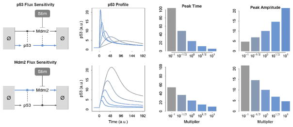
Special cases of isostatic perturbations are those that simultaneously alter the homeostatic rates of synthesis and degradation – or flux – of a particular species. Above we saw that changing the steady-state abundance of Mdm2 altered the flux of p53 and thereby its dynamic responsiveness. However, we can alter the flux of p53 without altering the steady-state abundance of Mdm2 as well. This is shown in Fig. 4. Similar to the subsection above, increasing the flux of p53 results in a faster, stronger response. Decreasing the p53 flux results in a slower, weaker response, and to a greater degree than observed when changing Mdm2 alone.

Fig. 4.

The effect of p53 and Mdm2 flux on the dynamic response of p53 to stimulation. At top, the flux of p53 is varied from 0.1 (light gray) to 10 (dark gray) times its nominal wildtype value. At bottom, the flux of Mdm2 is varied from 0.1 (light gray) to 10 (dark gray) times its wildtype vale. The effects of each on the time and amplitude of the p53 response are shown as bar graphs on the right. (For color version of this figure, the reader is referred to the web version of this book.)

In addition to p53, we can alter the homeostatic flux of the negative regulator, Mdm2. This is shown in Fig. 4, bottom. In contrast to p53, increasing the flux of Mdm2 results in a faster but weaker p53 response. This result highlights the fact that while the homeostatic flux of a species within a biochemical reaction or gene regulatory network can affect the dynamic response to perturbation, the precise nature of the effect depends on the function of that species within the network.

D. Precise Control of the Dynamic Response by Homeostatic Flux

The distinct effects of homeostatic p53 versus Mdm2 flux on the dynamic response of p53 raise the possibility that these fluxes can be used to precisely control the shape of the p53 trajectory. Using the time and amplitude of the peak of the p53 trajectory as descriptors of the shape, we can look for isostatic perturbations that affect the flux of both p53 and Mdm2 such that the peak time is altered independently of the amplitude, or the amplitude independently of the time.

In Fig. 5, we see that this is indeed possible. In fact, in Fig. 4 we can see that the p53 and Mdm2 fluxes have an equal but opposite effect on the peak amplitude. This suggests that an isostatic perturbation that pairs an increase in one flux with an equal but opposite decrease in the other will preserve the amplitude of p53. This is shown to be the case in Fig. 5 top. Since this same phenomenon is not manifested in the p53 peak time, it is less straightforward to derive the desired isostatic perturbation. However, given a particular change in Mdm2 flux, we can indeed find a change in p53 flux such that the p53 peak time is preserved (Fig. 5, bottom). Together, these results demonstrate that the dynamic response of p53 can be precisely controlled by homeostatic flux, independently of the steady-state abundances of either p53 or Mdm2.

Fig. 5.

Precise tuning of the dynamic response of p53 to stimulation by homeostatic flux. At top, the flux of p53 is varied from 0.1 (light gray) to 10 (dark gray) times its nominal wildtype value, while the flux of Mdm2 is varied from 10 (light gray) to 0.1 (times its wildtype value). The result of this modulation is that amplitude of the p53 response is held constant. At bottom, the flux of Mdm2 is varied from 0.1 (light gray) to 10 (dark gray) times its wildtype value. A modification to the flux of p53 is then derived numerically such that the time of the p53 response is held constant. (For color version of this figure, the reader is referred to the web version of this book.)

IV. Open Challenges

Because the assumptions of spatial homogeneity and high concentrations remain prevalent in the systems biology and modeling literature, we believe there is ample opportunity to use py-substitution to generate novel hypotheses about the impact of steady-state on stimulus responsiveness. Nevertheless, even within a mass action framework there are limitations to the method as described here. Chief among these is that of model size. Deriving symbolic bases for the solution space to the steady-state equation and isostatic subspace of a large model can yield elements with hundreds and sometimes thousands of terms. An attractive solution to this problem would be a priori identification of network modules (Bowsher, 2011; Hartwell et al., 1999). In the ideal case, this would result in block diagonal coefficient and Jacobian matrices. Since each block can be treated independently, the algebraic complexity of the resultant basis vectors would be much more manageable. Identifying modules would also offer the benefit of allowing some species to be in disequilibrium, as the case might be when a signaling network experiencing ambient, tonic signaling is coupled to a periodic oscillator such as the cell cycle.

For systems in which the assumptions for mass action are not supported, some work will have to be done to extend the py-substitution framework. For spatially heterogeneous systems, the mass balance equations include a diffusion term in addition to the standard mass action rate equations. It remains to be shown whether such a system of equations can be linearized in the same manner as described here. If indeed it can, this could lead to new insights regarding the interplay between reaction kinetics and diffusivity in establishing spatial gradients and responding to spatially heterogeneous signals. When the assumption of high concentrations is violated and a system loses its deterministic behavior, the inference of kinetic parameters from steady-state concentrations or dynamic response measurements becomes a probabilistic one. Additional work will be done to extend py-substitution to these stochastic systems.

More generally, the class of models that can be addressed using py-substitution remains to be determined. Are their structural motifs within a BRN that are particularly challenging to linearize? Can more exotic reaction rate equations be entertained, notably Michaelis–Menten kinetics and Hill functions? Precisely defining the domain of py-substitution will not only guide its further development, but perhaps also dissuade the use of exotic reaction kinetics to achieve a certain dynamical behavior, at the expense of a knowable steady-state.

V. Computational Methods

In this section, we give step-by-step instructions for identifying the steady-state of the p53 model. Although the size of this model makes it unnecessary to employ the rigorous treatment described here, that the results can be reproduced by hand makes the steps tractable and easy to follow. For information on how the method scales to larger models, see Loriaux et al., 2012. Once we identify a solution to the steady-state of the p53 model, we show how to derive a basis for its isostatic subspace. Finally, from the isostatic subspace we show how to derive specific isostatic perturbation vectors for modifying the homeostatic flux of p53 and Mdm2.

All of the steps below are performed using Matlab. As noted earlier, Matlab is not the best choice of software for symbolic calculations, but because it enjoys the most familiarity, we use it here for clarity. In the passages that follow, commands are identified by a double arrow prompt while output from the Matlab terminal is identified by a boldface font. Finally, it should be noted that the following code is in no way optimal; a more efficient implementation would make use of matrices, but again this efficiency comes at the expense of clarity.

A. Identifying an Expression for the Steady-state of a Mass Action Model

The p53 model consists of two species and four reactions. These must all be declared as symbolic variables using the syms keyword. Following convention, we use x to denote species, v for reaction velocities, and k for reaction rate constants. The real keyword identifies these variables as being real-valued. The semi-colon suppresses Matlab output.

By mass balance, we let the rate of change of each species be equal to the sum of reaction velocities in which that species is produced minus the sum of reaction velocities in which it is consumed. This yields the following.

Assuming mass action, we let the velocity of each reaction be equal to the product of its reactants and the corresponding rate constant.

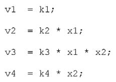
Substituting in the reaction velocities yields a system of mass balance equations expressed in terms of species and rate constants.

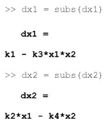
We must now linearize the system by imposing a py-substitution strategy. Even for a model of this size, several strategies exist. Here we’ll implement a strategy that assumes we have accurate measurements for the abundances of p53 and Mdm2 and the rate of p53 synthesis. The degradation rate constants and rate of Mdm2 synthesis will be left variable. Note that substituting for the rate of p53 synthesis requires the use of a pseudospecies, x3, which we introduce now.

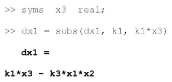
As before, we must declare all symbolic parameters and variables prior to substitution. Once a strategy is defined, we can use the same subs command to generate the py-substituted mass balance equations.

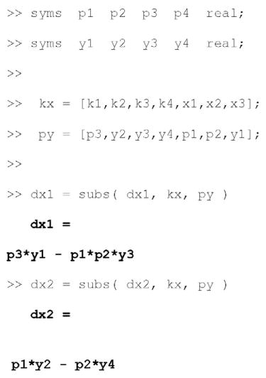
As expected, py-substitution results in a linear system of mass balance equations. As such, we can express it as the product between a coefficient matrix of parameters and a vector of variables. To derive the coefficient matrix, we use the jacobian command.

Now we’d like to find all vectors that, when left-multiplied by the coefficient matrix, equal zero. In other words, the vector must be in the null space of the coefficient matrix. To ensure this is true, we need to find a basis for the null space. This can be done using the null command. We’ll store the results of this operation in a second matrix, N.

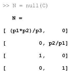
We now let the vector of variables equal any linear combination of column vectors in N. Because N has two columns, we’ll need two additional parameters, q1 and q2. These will be the coefficients of the null space basis vectors.

Next, we must resolve the pseudospecies such that its value is one. Since y1 is the variable that corresponds to the pseudospecies x3, this means we must find a value for q1 such that y1=1. Also note that the coefficient q2 maps to y4. This indicates that the rate constant k4 must in fact be a parameter. Here we will assume that this is not desirable, and that we would prefer to let the rate of Mdm2 synthesis be a parameter instead. To do this, we scale the second null space vector N(:,2) by a factor a2 such that N(2,:)*[q1;a2*q2]=q2.

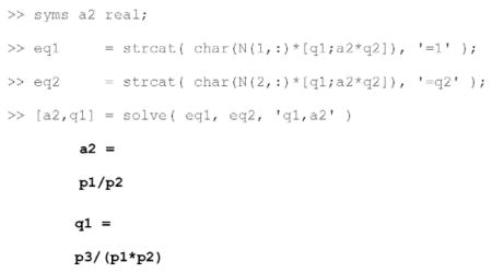
The final expression for the vector of variables is as follows.

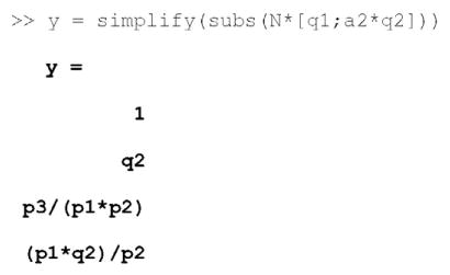
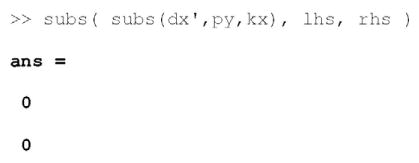
To be prudent, we verify that this vector is in the null space of the coefficient matrix.

Finally, we may wish to revert the substitution so that our steady-state expression is in terms of species and rate constants. Notice that the linear combination [q1;q2] effectively identifies variables that, because the coefficient matrix was underdetermined, turn out to be parameters. These variables map one-to-one with null space basis vector coefficients. Thus in our steady-state expression for y, to the left hand side we simply reverse the substitution from py back to kx. To the right hand side we first perform the one-to-one substitution from q to y, then the reverse substitution from py to kx.

The result of the inverse substitution is a relationship between dependent and independent species and rate constants that, if satisfied, guarantees steady-state. Note that this relationship is particular to our choice of py-substitution strategies and null space basis vector coefficients. As illustrated above, by scaling the appropriate basis vector, we were able to choose which variables remain dependent. Finally, it is worth verifying that our solution for y does indeed guarantee steady-state.

B. Identifying the Isostatic Subspace of a Mass Action Model

As illustrated in Figs. 2–4, there are many advantages to having an analytical expression for the steady-state of a mass action model: (a) static measurements of species abundances can be used to calculate kinetic rate constants, (b) the total number of parameters required is often reduced (Loriaux et al., 2012), and perhaps most importantly, (c) we can characterize the relationship between dynamic responsiveness and the abundances of species at steady-state. However, as seen in Fig. 3, steady-state abundances do not uniquely determine the dynamic response; the kinetics of the system are also important.

To study the effects of kinetics on dynamic responsiveness in isolation, we would like to identify any and all changes that can be made to the kinetic rate constants that do not alter the steady-state species abundances. The set of all such changes is called the isostatic subspace. To identify this subspace, it is first easier to return to the parametric description of the steady-state. At this point, we’ll also replace the null space basis vector coefficient q2 with the parameter, p4.

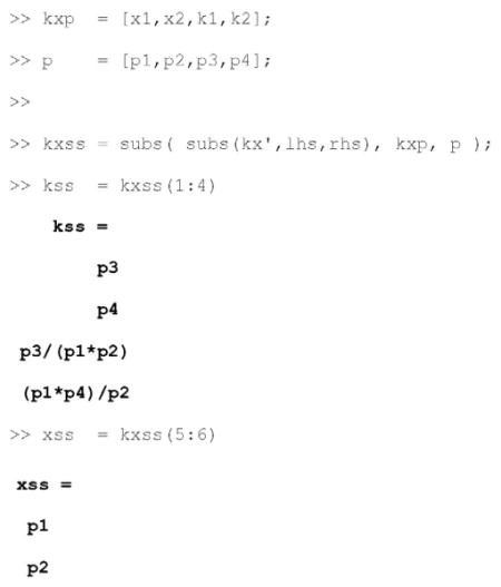
As expected, every element in our model is a function of the four parameters used in the py-substitution strategy. Now recall that a Taylor expansion can be used to approximate how these elements change in response to changes in parameters. The first order term of this expansion requires a matrix of partial derivatives of each element with respect to each parameter. This matrix is also called the Jacobian matrix, and can be calculated in Matlab using the jacobian command.

In the Jacobian Jx, the rows correspond to steady-state species abundances and the columns to parameters. Element Jx(1,1)=1 indicates that a change in parameter p1 results in an equal change in species x1. This of course is not surprising since our py-substitution strategy had that x1=p1. It is also not surprising that Jx(1,2)=Jx(1,3)=Jx(1,4)=0; the species x1 doesn’t depend on any other parameter. The second row of Jx has a similar structure; the species x2 depends only on the parameter p2. This Jacobian matrix is extraordinarily simple because both steady species abundances were modeled as independent parameters. In general, there will be species whose steady-state abundances are variable expressions of the parameters, and this significantly complicates the Jacobian.

It now remains to identify the set of all vectors that, when left multiplied by Jx, result in zero. By our Taylor expansion, any such vector identifies a change in parameters that results in no changes to the species abundances. By the same argument as above, any such vector must be in the null space of the Jacobian, and as before, a basis for this null space is found using the null command.

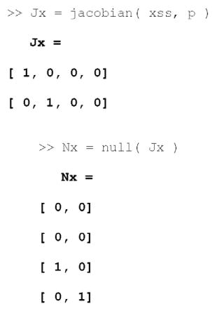
In this matrix, each row corresponds to a parameter and every column to a degree of freedom in the null space. That the first two rows are comprised entirely of zeros indicates that we can alter neither p1 nor p2 without altering at least one steady-state abundance. Again, this is not surprising since x1=p1 and x2=p2. The bottom two rows indicate that we can alter either p3or p4independently of one another. This too is not surprising; neither p3 nor p4 appear in the steady-state expressions for x1 and x2. As with the Jacobian matrix, the null space basis will typically have a more complicated expression.

To derive a general expression for the isostatic subspace of our p53 model, we take a linear combination of the null space basis vectors. The null space is two-dimensional so two coefficients are required, q1 and q2. And because we already used these variables in the previous subsection, we’ll clear them prior to using them again.

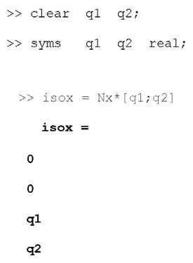
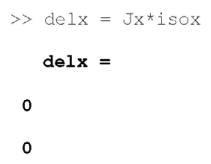
The vector isox states simply that we may make any change to the parameters p3 and p4 without altering the steady-state abundances x1 and x2. To verify that this is true, we map the parameter perturbation isox into a species abundance perturbation delx using the Jacobian, Jx. As expected, the parameter perturbation resides in the null space of the Jacobian, indicating that the perturbation causes no change in species abundances.

How does the general isostatic perturbation isox affect the rate constants of our model? And how do we identify a specific perturbation such that only certain rate constants are altered? To calculate the effect of the general perturbation isox on the set of rate constants we use the same procedure as above, but using the Jacobian matrix of rate constants with respect to the parameters instead of species abundances.

As we saw with Jx, the first two rows indicate that changes to p3 and p4 result in equivalent changes to k1 and k2, respectively. This simply reflects the fact that k1=p3 and k2=p4, and that our py-substitution strategy was designed to make the rates of synthesis of p53 and Mdm2 independent parameters. The degradation rate constants k3 and k4 are variable and constrained by steady-state, and are thus each sensitive to changes in three out of four parameters. The product of Jx and isox maps this perturbation into a change in rate constants.

As we observed in the Jacobian, a change q1 in parameter p3 results in an equivalent change in the rate constant k1. A change q2 in parameter p4 results in an equivalent change in k2. The resultant changes in the degradation rate constants, however, are scaled by the species abundances p1 and p2. We can calculate the vector of rate constants that results from the perturbation isox by executing the first sum in the Taylor expansion.

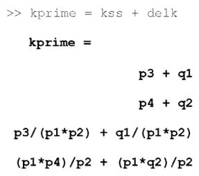
Finally, what if we are interested in not just any isostatic perturbation but a specific one? In Fig. 5, we saw that the homeostatic flux of p53 and Mdm2 can precisely control the dynamic response of p53 to DNA damage. Altering the homeostatic flux is just a special case of the general perturbation isox. We need only find values for q1 and q2 such that the rate constants k1 and k3 and k2 and k4 take on values theta1 and theta2 times their nominal wildtype values, respectively. To do this, we first declare the symbolic variables theta1 and theta2. We then express our desired outcome as a system of equations. Specifically, letting k1prime and k2prime be the altered values of k1 and k2, the ratio of the k1 prime to k1 should be theta1, and the ratio of k2 prime to k2 should be theta2. Once expressed as such, we can solve for the requisite values of q1 and q2.

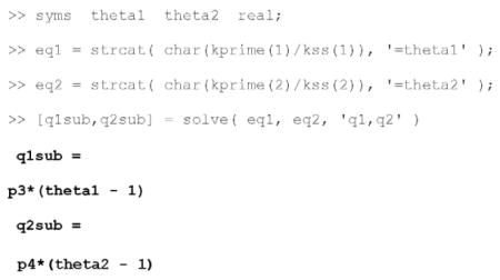
Substituting these values into the general isostatic perturbation isox results in the desired, specific isostatic perturbation that scales the homeostatic flux of p53 and Mdm2.

Finally, it remains to verify that this perturbation results in the desired change. Again this is done by executing the first sum in the Taylor expansion.

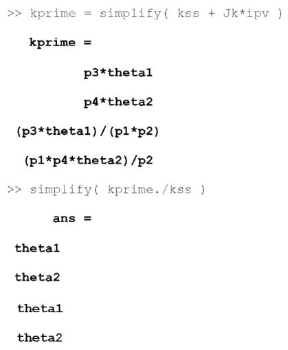
In summary, from the parametric expression for the steady-state of our model, we have identified a specific isostatic perturbation that alters the homeostatic flux of either or both p53 and Mdm2 to the user-specified parameters theta1 and theta2, respectively.

VI. Further Reading

Another method for deriving expressions for the steady-states of mass action models was introduced by King and Altman in 1956 (King and Altman, 1956). This graphical method was greatly improved upon in Volkenstein and Goldstein (1966) and again in Thomson and Gunawardena (2009), and enjoys a robust and sophisticated implementation in Matlab (Qi et al., 2009).

The application of linear algebra to dynamical networks has a similarly rich history, especially as it pertains to flux balance analysis (Gianchandani et al., 2010) and systems biology (Palsson, 2006). For a deeper understanding of the relevant concepts in linear algebra, see Poole (2010) and Cooperstein (2010).

Evaluating the effects of perturbations on network dynamics and steady-state has long been the subject of metabolic control analysis, or MCA (Heinrich and Rapoport, 1974; Fell, 2005). Succinctly, MCA can be used to quantify the steady-state change in a reaction velocity or species concentration due to a change in an independent parameter. Recently this framework was extended to dynamical states as well (Ingalls and Sauro, 2003). For an excellent review of quantitative modeling of network dynamics, see Sauro (2009).

References

- Bartlett DW, Davis ME. Insights into the kinetics of siRNA-mediated gene silencing from live-cell and live-animal bioluminescent imaging. Nucleic Acids Res. 2006;34:322–333. doi: 10.1093/nar/gkj439. [DOI] [PMC free article] [PubMed] [Google Scholar]
- Becker V, Schilling M, Bachmann J, Baumann Raue A, Maiwald T, Timmer J, Klingmüller U. Covering a broad dynamic range: information processing at the erythropoietin receptor. Science. 2010;328:1404–1408. doi: 10.1126/science.1184913. [DOI] [PubMed] [Google Scholar]
- Bowsher CG. Automated analysis of information processing, kinetic independence and modular architecture in biochemical networks using MIDIA. Bioinformatics. 2011;27:584–586. doi: 10.1093/bioinformatics/btq694. [DOI] [PubMed] [Google Scholar]
- Cooperstein B. Advanced Linear Algebra. Vol. 1. CRC Press; 2010. p. 364. [Google Scholar]
- Dolloff NG, Mayes PA, Hart LS, Dicker DT, Humphreys R, El-Deiry WS. Off-target lapatinib activity sensitizes colon cancer cells through TRAIL death receptor up-regulation. Sci Transl Med. 2011;3:86ra50. doi: 10.1126/scitranslmed.3001384. [DOI] [PMC free article] [PubMed] [Google Scholar]
- Faller D, Klingmuller U, Timmer J. Simulation methods for optimal experimental design in systems biology. Simulation. 2003;79:717–725. [Google Scholar]
- Fell D. Metabolic control analysis. In: Alberghina L, Westerhoff HV, editors. Systems Biology. Springer; Berlin/Heidelberg: 2005. pp. 397–424. [Google Scholar]
- Fire A, Xu S, Montgomery MK, Kostas SA, Driver SE, Mello CC. Potent and specific genetic interference by double-stranded RNA in Caenorhabditis elegans. Nature. 1998;391:806–811. doi: 10.1038/35888. [DOI] [PubMed] [Google Scholar]
- Fulda S, Küfer MU, Meyer E, van Valen F, Dockhorn-Dworniczak B, Debatin KM. Sensitization for death receptor- or drug-induced apoptosis by re-expression of caspase-8 through demethylation or gene transfer. Oncogene. 2001;20:5865–5877. doi: 10.1038/sj.onc.1204750. [DOI] [PubMed] [Google Scholar]
- Fulda S, Meyer E, Debatin K. Inhibition of TRAIL-induced apoptosis by Bcl-2 over-expression. Oncogene. 2002;21:2283–2294. doi: 10.1038/sj.onc.1205258. [DOI] [PubMed] [Google Scholar]
- Gianchandani EP, Chavali AK, Papin JA. The application of flux balance analysis in systems biology. Wiley Interdiscip Rev Syst Biol Med. 2010;2:372–382. doi: 10.1002/wsbm.60. [DOI] [PubMed] [Google Scholar]
- Gillespie D. A rigorous derivation of the chemical master equation. Physica A. 1992;188:404–425. [Google Scholar]
- Grima R, Schnell S. Modeling reaction kinetics inside cells. Essays Biochem. 2008;45:41–56. doi: 10.1042/BSE0450041. [DOI] [PMC free article] [PubMed] [Google Scholar]
- Hartwell LH, Hopfield JJ, Leibler S, Murray AW. From molecular to modular cell biology. Nature. 1999;402:C47–C52. doi: 10.1038/35011540. [DOI] [PubMed] [Google Scholar]
- Heinrich R, Rapoport TA. A linear steady-state treatment of enzymatic chains. Critique of the crossover theorem and a general procedure to identify interaction sites with an effector. Eur J Biochem. 1974;42:97–105. doi: 10.1111/j.1432-1033.1974.tb03319.x. [DOI] [PubMed] [Google Scholar]
- Hinz S, Trauzold A, Boenicke L, Sandberg C, Beckmann S, Bayer E, Walczak H, Kalthoff H, Ungefroren H. Bcl-XL protects pancreatic adenocarcinoma cells against CD95- and TRAIL-receptor-mediated apoptosis. Oncogene. 2000;19:5477–5486. doi: 10.1038/sj.onc.1203936. [DOI] [PubMed] [Google Scholar]
- Ingalls BP, Sauro HM. Sensitivity analysis of stoichiometric networks: an extension of metabolic control analysis to non-steady state trajectories. J Theor Biol. 2003;222:23–36. doi: 10.1016/s0022-5193(03)00011-0. [DOI] [PubMed] [Google Scholar]
- Itzkovitz S, van Oudenaarden A. Validating transcripts with probes and imaging technology. Nat Methods. 2011;8:S12–S19. doi: 10.1038/nmeth.1573. [DOI] [PMC free article] [PubMed] [Google Scholar]
- Izant JG, Weintraub H. Inhibition of thymidine kinase gene expression by anti-sense RNA: a molecular approach to genetic analysis. Cell. 1984;36:1007–1015. doi: 10.1016/0092-8674(84)90050-3. [DOI] [PubMed] [Google Scholar]
- Jain A, Liu R, Ramani B, Arauz E, Ishitsuka Y, Ragunathan K, Park J, Chen J, Xiang YK, Ha T. Probing cellular protein complexes using single-molecule pull-down. Nature. 2011;473:484–488. doi: 10.1038/nature10016. [DOI] [PMC free article] [PubMed] [Google Scholar]
- Kearns JD, Hoffmann A. Integrating computational and biochemical studies to explore mechanisms in NF-κB signaling. J Biol Chem. 2009;284:5439–5443. doi: 10.1074/jbc.R800008200. [DOI] [PMC free article] [PubMed] [Google Scholar]
- Kholodenko BN. Spatially distributed cell signalling. FEBS Lett. 2009;583:4006–4012. doi: 10.1016/j.febslet.2009.09.045. [DOI] [PMC free article] [PubMed] [Google Scholar]
- Kim J-Y, Lee J-Y, Kim D-G, Koo G-B, Yu J-W, Kim Y-S. TRADD is critical for resistance to TRAIL-induced cell death through NF-κB activation. FEBS Lett. 2011;585:2144–2150. doi: 10.1016/j.febslet.2011.05.034. [DOI] [PubMed] [Google Scholar]
- King EL, Altman C. A schematic method of deriving the rate laws for enzyme-catalyzed reactions. J Phys Chem. 1956;60:1375–1378. [Google Scholar]
- Kitano H. Systems biology: a brief overview. Science. 2002;295:1662–1664. doi: 10.1126/science.1069492. [DOI] [PubMed] [Google Scholar]
- Li H, Cao Y, Petzold LR, Gillespie DT. Algorithms and software for stochastic simulation of biochemical reacting systems. Biotechnol Prog. 2011;24:56–61. doi: 10.1021/bp070255h. [DOI] [PMC free article] [PubMed] [Google Scholar]
- Loriaux PM, Tesler G, Hoffmann H. An algebraic method for deriving analytical expressions for steady states of mass action models. 2012 doi: 10.1371/journal.pcbi.1002901. Submitted. [DOI] [PMC free article] [PubMed] [Google Scholar]
- Nutiu R, Friedman RC, Luo S, Khrebtukova I, Silva D, Li R, Zhang L, Schroth GP, Burge CB. Direct measurement of DNA affinity landscapes on a high-throughput sequencing instrument. Nat Biotechnol. 2011;29:659–664. doi: 10.1038/nbt.1882. [DOI] [PMC free article] [PubMed] [Google Scholar]
- O’Dea EL, Kearns JD, Hoffmann A. UV as an amplifier rather than inducer of NF-kappaB activity. Mol Cell. 2008;30:632–641. doi: 10.1016/j.molcel.2008.03.017. [DOI] [PMC free article] [PubMed] [Google Scholar]
- Palsson BØ. Systems Biology: Properties of Reconstructed Networks. Cambridge University Press; 2006. p. 334. [Google Scholar]
- Poole D. Linear Algebra: A Modern Introduction. Vol. 3. Brooks Cole; 2010. p. 768p. [Google Scholar]
- Qi F, Dash RK, Han Y, Beard DA. Generating rate equations for complex enzyme systems by a computer-assisted systematic method. BMC Bioinformatics. 2009;10:238. doi: 10.1186/1471-2105-10-238. [DOI] [PMC free article] [PubMed] [Google Scholar]
- Reynolds A, Anderson EM, Vermeulen A, Fedorov Y, Robinson K, Leake D, Karpilow J, Marshall WS, Khvorova A. Induction of the interferon response by siRNA is cell type-and duplex length-dependent. RNA. 2006;12:988–993. doi: 10.1261/rna.2340906. [DOI] [PMC free article] [PubMed] [Google Scholar]
- Sauro HM. Network Dynamics. In: Ireton R, Montgomery K, Bumgarner R, Samudrala R, McDermott J, editors. Computational Systems Biology. Humana Press; Totowa, NJ: 2009. pp. 269–309. [Google Scholar]
- Schwanhäusser B, Busse D, Li N, Dittmar G, Schuchhardt J, Wolf J, Chen W, Selbach M. Global quantification of mammalian gene expression control. Nature. 2011;473:337–342. doi: 10.1038/nature10098. [DOI] [PubMed] [Google Scholar]
- Slepchenko BM, Schaff JC, Carson JH, Loew LM. Computational cell biology: spatiotemporal simulation of cellular events. Annu Rev Biophys Biomol Struct. 2002;31:423–441. doi: 10.1146/annurev.biophys.31.101101.140930. [DOI] [PubMed] [Google Scholar]
- Sreenath SN, Cho K-H, Wellstead P. Modelling the dynamics of signalling pathways. Essays Biochem. 2008;45:1–28. doi: 10.1042/BSE0450001. [DOI] [PubMed] [Google Scholar]
- Tanious FA, Nguyen B, Wilson WD. Biosensor-surface plasmon resonance methods for quantitative analysis of biomolecular interactions. Methods Cell Biol. 2008;84:53–77. doi: 10.1016/S0091-679X(07)84003-9. [DOI] [PubMed] [Google Scholar]
- Thomson M, Gunawardena J. The rational parameterization theorem for multisite post-translational modification systems. J Theor Biol. 2009;261:626–636. doi: 10.1016/j.jtbi.2009.09.003. [DOI] [PMC free article] [PubMed] [Google Scholar]
- Volkenstein M, Goldstein B. A new method for solving the problems of the stationary kinetics of enzymological reactions. Biochim Biophys Acta. 1966;115:471–477. [Google Scholar]
- Zhang L, Fang B. Mechanisms of resistance to TRAIL-induced apoptosis in cancer. Cancer Gene Ther. 2005;12:228–237. doi: 10.1038/sj.cgt.7700792. [DOI] [PubMed] [Google Scholar]