Functional vs. Traditional Analysis in Biomechanical Gait Data: An Alternative Statistical Approach

Abstract

In human motion studies, discrete points such as peak or average kinematic values are commonly selected to test hypotheses. The purpose of this study was to describe a functional data analysis and describe the advantages of using functional data analyses when compared with a traditional analysis of variance (ANOVA) approach. Nineteen healthy participants (age: 22 ± 2 yrs, body height: 1.7 ± 0.1 m, body mass: 73 ± 16 kg) walked under two different conditions: control and pain+effusion. Pain+effusion was induced by injection of sterile saline into the joint capsule and hypertonic saline into the infrapatellar fat pad. Sagittal-plane ankle, knee, and hip joint kinematics were recorded and compared following injections using 2×2 mixed model ANOVAs and FANOVAs. The results of ANOVAs detected a condition × time interaction for the peak ankle (F1,18 = 8.56, p = 0.01) and hip joint angle (F1,18 = 5.77, p = 0.03), but did not for the knee joint angle (F1,18 = 0.36, p = 0.56). The functional data analysis, however, found several differences at initial contact (ankle and knee joint), in the mid-stance (each joint) and at toe off (ankle). Although a traditional ANOVA is often appropriate for discrete or summary data, in biomechanical applications, the functional data analysis could be a beneficial alternative. When using the functional data analysis approach, a researcher can (1) evaluate the entire data as a function, and (2) detect the location and magnitude of differences within the evaluated function.

Introduction

In order to study movement, adaptations to movement and movement intervention, large sets of biomechanic, neurologic and physiologic data must be collected and interpreted. This process can be difficult and many limitations can impede it. The statistical approach for analyzing these data sets can be one of these limitations. For example, joint angles during movement have been compared using various statistical analyses such as t-tests (Powers et al., 2012), analyses of variance (ANOVA) (Torry et al., 2000) and covariance (Carneiro et al., 2012), and multivariate analyses of variance (Mundermann et al., 2005). These traditional statistical approaches are sound, but limited in a similar way. An ANOVA can only provide information regarding a discrete time point (e.g., peak knee flexion) or grouping of points (e.g., mean knee flexion) that were involved in the movement or a part of the movement.

While an ANOVA only provides information regarding a discrete data point(s), a functional data analysis considers entire functions (Ramsay and Silverman, 2005). More specifically, a functional data analysis can be used to compare condition effects on entire time functions (e.g., the entire stance phase of the gait) (Hopkins et al., 2012). In this way, a functional data analysis may be more informative, relative to other statistical approaches that analyze discrete points in time, because a functional data analysis can compare all collected data as functions. A functional data analysis may detect whether a difference exists, multiple differences over time, the magnitude and meaningfulness of the difference, and when statistical differences occur in time. A functional data analysis may result in a plot showing mean differences and corresponding effect sizes, plotted against the “normal” time function.

The purpose of this technical report is to describe the value of a functional data analysis in analyzing joint angles (in the sagittal plane) during walking. We analyzed these data using a functional linear model and a more traditional approach (ANOVA). The data reported here were collected for a study that was conducted to better understand neuromechanical alterations due to experimental knee effusion and pain in ablebodied participants. We chose to report sagittal plane joint kinematics because they are commonly measured and reported in the biomechanical literature (Nadeau et al., 1997; Sulzer et al., 2010).

Methods

Participants and Procedures

Nineteen able-bodied participants (10 males and 9 females; age: 22 ± 2 yrs; body height: 1.73 ± 0.10 m; body mass: 73 ± 16 kg) arrived at the lab, gave informed consent approved by the University’s Review Board, and were prepared for motion analysis. For this study, we determined joint angles using previously described methods (Seeley et al., 2013), except that, presently, we calculated the hip joint center using a functional approach (Schwartz and Rozumalski, 2005). Participants completed the pre-injection walking trials (all walking trials were performed at a selfselected speed). Next, participants received one of the conditions (pain+effusion or control/no injection). To induce pain and effusion, we used the common injury models of pain (Park and Hopkins, 2013) and effusion (Hopkins et al., 2002). The post-injection walking trials were performed five minutes following the last injection. Three walking trials were recorded under each condition and all trials were used in analysis. The spatial coordinates for each reflective marker were determined and tracked using Vicon Nexus 1.7 (Vicon, Centennial, CO, USA) and then exported to Visual3D (C Motion, Germantown, MD, USA). The data were smoothed using a 4^th-order low-pass Butterworth filter with a cut off frequency of 6 Hz (Hunt et al., 2010).

Statistical Analyses

To test condition effect over time, we performed five separate 2×2 ANOVAs for peak ankle dorsiflexion, ankle plantarflexion, knee flexion, hip flexion, and hip extension angles throughout stance (SAS 9.3, SAS Institute Inc., Cary, NC, USA). Tukey-Kramer post-hoc tests were carried out for post-hoc comparisons (p = 0.05). We also conducted three separate functional analyses for the sagittal plane ankle, knee and hip joint angles (R 2.15.1, R development core team, http://madison.byu.edu/FDA.html). We used a modified version of a functional data analysis procedure (Andrade et al., 2014). This requires use of basis functions, warping and a statistical framework, as described below.

Key Applications

In order to better understand the functional data analysis process, we will detail some of the steps. First the data must be defined in terms of curve or function characteristics (reparameterization). Next the data are warped or time registered. Finally the data are fit to a model for hypothesis testing.

Re-parameterization using Basis Functions

A functional data analysis allows us to compare functional responses over time. The first step in a functional data analysis is to identify a set of characteristics that are comparable from curve to curve. Curves are re-parameterized using basis functions. A basis representation of a curve consists of a set of basis functions and corresponding set of weights. The weighted sum of the basis functions yields the original curve.

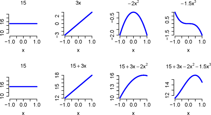
An example of a curve is created using basis functions {1,x,x²,x³} with weights {15, 3, –2, –1.5}, resulting in the polynomial f(x) = 15 + 3x – 2x² – 1.5x³ (Figure 1). Choosing the number of basis functions to represent any given curve and the corresponding weights is a difficult estimation problem. For instance, in the bottom right plot in Figure 1, if we considered only functions (1, x, x²}, the representation of the original curve would not have been exact (as seen in the plot in the bottom row, 3^rd column in Figure 1). While suitable for some simpler curves, polynomials are not as flexible as other choices (Ramsay and Silverman, 2005).

Figure 1.

The top row of plots shows the weighted basis functions and the bottom row shows those functions added together, one by one, to represent the original curve. That basis functions are functions of the same inputs as the function they are being used to represent (functions of time in the present case).

One example of a more flexible choice is a spline basis. A spline is formed by splitting the domain (the possible x values of f(x)) of a curve into pieces and representing the corresponding pieces of the curve with local polynomial functions. Cubic polynomials are often sufficient, resulting in a cubic spline. Constraints can be employed to assure that the pieces fit together smoothly.

More formally, a basis function representation of a function f can be written as $\begin{array}{l}f(x)=\sum _{i=1}^p{h}_i(x){\beta }_i\end{array}$

where h_i(x)) is a basis function, β_i is the corresponding weight and p is the number of basis functions. Say we choose to break the domain of a curve into j pieces (the locations of the breaks we call knots). Then we can fit a cubic spline to the curve by letting the basis functions be:

$$\begin{array}{c}{h}_1(x)=1\\ h_2(x)=x\\ h_3(x)=x^2\\ h_4(x)=x^3\\ h_5(x)=(x-k_1{)}^{3}I(x\ge k_1)\\ h_6(x)=(x-k_2{)}^{3}I(x\ge k_2)\\ :\\ h_{j+4}(x)=(x-k_j{)}^{3}I(x\ge k_j)\end{array}$$

and fitting the linear model

$$\begin{array}{c}{\displaystyle \sum _{i=1}^p{h}_i(x){\beta }_i+\epsilon }\end{array}$$

to find the weights. Here I is the indicator function (1 if the argument is true and 0 otherwise), k is a particular knot, y is f(x) and ε is the model error. This choice of basis functions ensures that the resulting function will be smooth.

Now, consider a function not as easily represented with a polynomial (Figure 2). Fitting a cubic spline to this curve with 10 equally spaced knots (equally spaced from each other and the start and end points of these data, which are -1 and 1) yields a reasonable fit to the data. The basis functions and their cumulative weighted sum are shown in Figure 3.

Figure 2.

Polynomial curves to represent a function The curve in the left column plot is more representative of the type of the stance phase curve we are considering. However, the stance phase data we actually observe and use to fit curves are discrete, which may look more like the curve in the right column plot.

Figure 3.

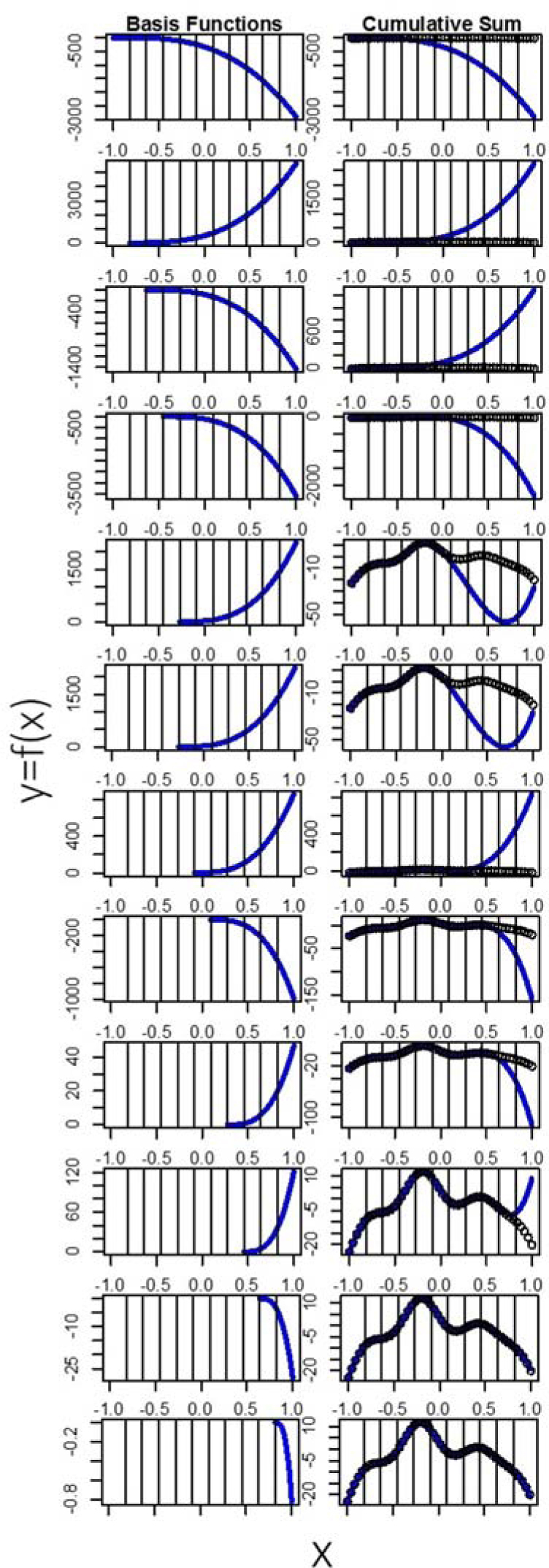
Basis functions and cumulative sum These figures explain the sum of basis functions one at a time, sequentially. The first row of the plot shows the first four basis functions added together with the fitted weights. The left side of the next 10 rows shows the basis functions that involve the 10 knots. The right side of the next 10 rows shows the cumulative sum of this basis functions. By the time we add the 10^th basis function, we have successfully represented our data with a curve.

An important step in a functional data analysis is to time register or warp the data. Time registering entails aligning in time specific landmarks in each function. This can reduce noise (due to time differences between each participants’ walking) observed in the x-axis of the functions, allowing for the often more relevant y-axis variation to be better analyzed. Landmarks often include peaks, valleys, and the start and end points (Ramsay and Silverman, 2005). For some biomechanical data, these landmarks could correspond to events like initial contact or toe-off. After choosing landmarks, we transform the data so that the landmarks occur at roughly the same points in time within the stance phase. To transform the data, we fit warping functions, which have as inputs the location of the landmarks (in the stance phase) before warping and output the location of the landmarks after warping. Using linear functions, we smoothed over the rest of the stance phase around the landmarks. Thus, using these warping functions, we can transform data to have landmarks occur at similar points in time and have the rest of the data match the pattern accordingly.

Problems may arise when using landmark registration. Landmark analysis warps the input space of the functions, often making them less interpretable. In order to make these functions of percent stance phase an interpretable quantity, in this analysis we chose initial contact and toe-off in the stance phase as the start and end points for landmarks (Figure 4). We then transformed each function to have the same start and end points using a line through the two chosen landmarks.

Figure 4.

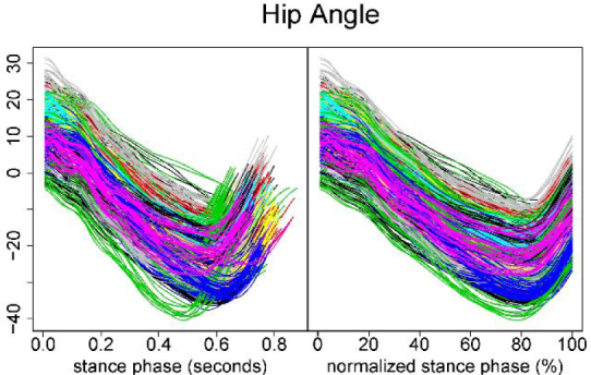
Raw and time-normalized kinematic data for the hip joint The left column plot represents the raw kinematic data for the hip joint. The right column plot represents the time-normalized data. Note that each function (trace) has different end points. The right column plot represents time registration using the two chosen landmarks (start and end points).

After time registering these data, we used a B-spline basis with 19 basis functions to represent each curve in the dataset. B-splines are a more stable and computationally efficient basis than cubic splines, and any cubic spline basis can be represented with B-splines (De Boor, 1972). This means that each curve in the dataset is composed of the same 19 basis functions (weighted and added together), though the weights are allowed to vary from curve to curve. In order to perform a functional data analysis, we statistically analyze these weights.

Consider the traditional two factor ANOVA model

$$\begin{array}{l}{y}_{ijk}=\mu +{\alpha }_j+{\beta }_k+\alpha {\beta }_{jk}+{\epsilon }_{ijk}\end{array}$$

where α_j is the factor one level j effect, β_k is the factor 2 level k effect, αβ_jk is the interaction between these two factors at the prescribed levels, and μ is the overall mean. The two factor functional data analysis equivalent is

$$\begin{array}{l}{y}_{ijk}(t)=\mu (t)+{\alpha }_j(t)+{\beta }_k(t)+\alpha {\beta }_{jk}(t)+{\epsilon }_{ijk}(t)\end{array}$$

where t is time (percent stance phase in this case). Thus, the data and each effect in the model are functions of time. Similarly, the standard errors for each of the fitted effects are functions of time. We are particularly interested if there was an interaction (and main effect) as well as the pairwise comparisons of the model effects, which is to say we are interested in

$$\begin{array}{l}\alpha {\beta }_{1k}(t)-\alpha {\beta }_{2k}(t)\\ \alpha {\beta }_{2k}(t)-\alpha {\beta }_{3k}(t)\\ \alpha {\beta }_{1k}(t)-\alpha {\beta }_{3k}(t)\end{array}$$

etc. for each level of k and

$$\begin{array}{l}\alpha {\beta }_{j1}(t)-\alpha {\beta }_{j2}(t)\\ \alpha {\beta }_{j2}(t)-\alpha {\beta }_{j3}(t)\\ \alpha {\beta }_{j1}(t)-\alpha {\beta }_{j3}(t)\end{array}$$

etc. for each level of j. These are the differences between interactions that are meaningful. We plot our estimates of these pairwise comparison functions as well as 95% confidence bands to determine significance. If these confidence bands do not cross the zero line, we consider the difference significant.

Results

Using a traditional ANOVA approach, we found interactions in ankle plantarflexion (F_1,18 = 8.56, p = 0.001) and hip extension (F_1,18 = 5.77, p = 0.03). Under the pain+effusion condition, participants walked with 2° less peak dorsiflexion (p = 0.008) and 2.5° less peak hip extension (p = 0.02) compared to the pre-injection measurement. There was no difference in knee flexion angles (Table 1). The original kinematic data of the control group at post-injection measurements are presented in the left column of Figure 5.

Table 1.

Means (SD) for Peak Sagittal Plane Joint Angles During the Stance Phase of Walking.

		Condition		Results of 2 × 2 ANOVA and post-hoc comparisons
Variable	Time	Control	Pain+effusion
Hip flexion (°)	Pre			F1,18 = 0.32, p = 0.58
		13.23 (6.20)	11.81 (5.33)
	Post
		12.54 (6.99)	11.64 (6.18)
Hip extension (°)*	Pre			F1,18 = 5.77, p = 0.03; (Pre vs. Post in PE: p = 0.02)
		23.98 (6.84)	24.62 (5.95)
	Post
		23.97 (7.32)	22.11 (6.85)
Knee flexion (°)	Pre			F1,18 = 0.36, p = 0.56
		53.48 (2.55)	52.40 (4.44)
	Post
		54.16 (3.01)	52.47 (4.80)
Ankle dorsiflexion (°)	Pre			F1,18 = 0.04, p = 0.84
		12.56 (4.28)	12.51 (4.20)
	Post
		12.49 (4.51)	12.59 (4.56)
Ankle plantarflexion (°)*	Pre			F1,18 = 8.56, p = 0.01; (Pre vs. Post in PE: p = 0.01)
		16.95 (5.79)	16.94 (5.79)
	Post
		17.24 (5.70)	14.25 (5.63)

Pre: pre-injection; Post: post-injection; PE: pain+effusion Asterisks indicate condition × time interactions. A post-hoc test revealed that peak ankle plantarflexion and hip extension decreased due to the pain+effusion condition, relative to the pre-injection measurement.

Figure 5.

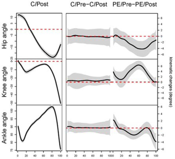
Results of functional data analyses in kinematic data The left column plots represent the original kinematic data for each joint. These data were used to choose peak angles for ANOVAs. The middle and right columns are the results of each FANOVA. We compared the joint angle between the time intervals (pre- and post-injection) for both conditions. For example, ankle angle C/Pre – C/Post (the middle plot at the bottom row) represents the mean difference between the pre- and post-injection measurement under the control condition.The x-axes represent percent of stance (from heel strike to toe-off). The y-axis for the left column epresents the mean function degrees while the y-axes for the middle and right column represent the mean difference in the ankle joint angle measured in degrees. The black line represents the average of differences between two time intervals (Pre and Post). When the 95% confidence bands (the shaded area) do not cover the zero line, a statistical between-time difference exists. For the ankle angle, during the pain+effusion condition, the injections caused subjects to walk with 2 ° less dorsiflexion at initial contact (0-5%), 2 ° greater dorsiflexion through the mid-stance (40-60%), and 4° less dorsiflexion at toe off (90-100%). For the knee angle, subjects after injections walked with 4 ° greater knee flexion at initial contact (0-5%: 4°) and 6 ° less knee extension approximately between 30-90% of the stance phase. For the hip angle, injections caused subjects to walk with 4 ° less hip extension approximately between 40-85% of the stance phase. C: control; PE: pain+effusion; Pre: pre-injection; Post: post-injection

(Insert Table 1 here)

According to the results of functional analyses, the pain+effusion condition resulted in participants walking with 2° less dorsiflexion at initial contact (0-5% of the stance), 2° greater dorsiflexion in the mid-stance (40-60% of the stance), and 4° less dorsiflexion at toe off (90-100%; Figure 5) compared to the pre-injection measurement. For the knee angle, participants under pain+effusion walked with 4° greater knee flexion at initial contact (0-5%) and 6° greater knee flexion between 30-90% of the stance phase compared to the pre-injection measurement (Figure 5). For the hip angle, participants under pain+effusion condition walked with 4° less hip extension between 40-85% of the stance phase compared to the pre-injection measurement (Figure 5).

Discussion

The purpose of this technical report was to describe the potential value of a functional data analysis in evaluating joint kinematics during walking. Using ANOVAs, we discovered a condition × time interaction for the peak ankle and hip joint angle, and subsequently detected between-time differences in peak ankle plantarflexion and peak hip extension for the pain+effusion condition. In comparison to the ANOVA, the results of functional data analysis revealed between-time differences at initial contact (ankle and knee joint), in the mid-stance (each joint) and at toe off (ankle joint). Furthermore, with mean difference functions surrounded by 95% confidence intervals (Figure 5), an estimation of effect size was also included for interpretation.

Analysis of an ensemble of curves and other comparisons of data over time is not a completely novel concept, but the application strength and sophistication used in the analysis varies. A recent paper describing a functional data analysis of variance approach (FANOVA) also used B-spline basis functions (Andrade et al., 2014). This paper proposed the simple effects model with one factor, as in y_jy(t) = μ(t) + α_j(t) + ε_jy(t), where μ(t) is the overall functional mean and is the effect of the jth level of Factor A. Our approach considers a cell means model version of this approach that allows for a more general treatment structure (two or more factors), meaning multiple independent variables can be used in the model. A summary of our model is:y_ijk(t)=μ_ij(t)+ε_ijk(t), where the effects of Factor A (subscript i) and the effects of Factor B (subscript j) are allowed to interact with each other.

Functional main effects and individual functional interaction effects can be estimated by constructing functional linear combinations of the cell means.

Other previously reported studies looking at data over time (Chicote et al., 2013; Mallor et al., 2010; Prosser et al., 2010; Ryan et al., 2006; Schollhorn et al., 2002) provide useful insights about the structure of the data using functional principle component analysis (PCA). PCA is used to describe the structure of data, not for making inference (p-value or confidence interval). The methods used in this paper (functional data analysis) yield additional insight via statistical inference, from which we obtain confidence bands and thus decide if treatments yield statistically different outcomes. The results of functional analyses specify where the differences exist in the stance phase, thus our data clearly describe some of the advantages of using functional analyses in joint kinematics when compared with typical ANOVAs.

Advantages of Functional Analyses

A functional data analysis is capable of detecting differences at any point in time, throughout the entire stance phase (or any other defined human motion). In comparison, while using ANOVA to evaluate differences, researchers could potentially fail to detect existing differences between discrete values if the differences do not occur precisely at the time of statistical evaluation (in this case, at the time of peak angle). Within the present data set, for example, participants demonstrated increased dorsiflexion throughout 40-60% of the stance after injections, relative to the pre-injection measurement. Relative to the results of the ANOVA, this finding is more informative as kinematic values between 40-60% of the stance phase are not often selected for analysis because peak dorsiflexion and plantarflexion do not typically occur during part of the stance phase.

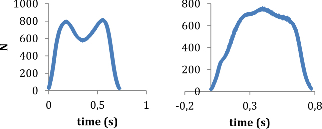
The characteristics of a curve (peaks, valleys, amplitudes, times, etc.) provide very useful information about the entire stance phase, therefore providing meaningful results that would not otherwise be observed. Figure 6 shows a representative function for ground reaction forces (GRF) prior to and after injection. Changes in the vertical ground reaction force during the unloading phase of gait, due to pain+effusion (Figure 6) demonstrate the value of a functional data analysis, relative to ANOVA. These GRF data were simultaneously recorded with the kinematic data reported in this paper. Before injection (Figure 6A), the GRF appears to be typical and there are distinct discrete points: peak impact, unloading and push-off. However, following injection (Figure 6B), the GRF appears to be altered as a result of the intervention (pain + effusion). In this case, an analysis of peak or mean GRF would likely not capture a significant difference due to pain+effusion; however a functional data analysis would capture the difference in functions, providing important information about where and how the GRF changes over time within the framework of a statistical model.

Figure 6.

Sample traces of vertical ground reaction forces during walking (a sample mean of a subject)The left and right column plot represents the data prior to and post injection, respectively. The injection appears to have significantly altered vertical ground reaction force during the stance phase of walking.

Limitation of Functional Analysis

While the application of a functional data analysis is very appealing, statistical modeling can be very complex and difficult to understand. Those who wish to incorporate a functional data analysis in exercise science related research will likely need to consult with someone who has experience in this area. Furthermore, not all data suit themselves to a functional approach. Data which are collected over time could be best for a functional data analysis.

Conclusion

We introduced a functional data analysis statistical approach for analyzing data collected over time and compared the results to those of a traditional ANOVA approach. The functional data analysis approach considers all collected data in a meaningful way. While the ANOVA detected differences in ankle plantarflexion and hip extension, the functional data analysis detected many differences throughout the entire stance phase in all joints, providing qualifying information about the data. Although in many situations, a traditional ANOVA is appropriate, in some biomechanical applications, the FANOVA could be a beneficial alternative.

What does this article add?

We introduced and explained the key applications of a functional data analysis for human movement data. The functional data analysis procedure used here is a modification of the previous model (Andrade et al., 2014). Our approach considers a more general cell means model version of the previous approach that allows for a general treatment structure of multiple factors.

Although a traditional ANOVA is often appropriate, in some biomechanical applications a functional data analysis could be a beneficial alternative. A functional data analysis approach considers all collected data in a meaningful way. When using a functional data analysis approach, a researcher can (1) evaluate and consider the entire data set as a function, and (2) detect the location and magnitude of differences within the evaluated function.

References

- Andrade AG, Polese JC, Paolucci LA, Menzel HJ, Teixeira-Salmela LF. Functional data analyses for the assessment of joint power profiles during gait of stroke subjects. J Appl Biomech. 2014;30:348–352. doi: 10.1123/jab.2013-0147. [DOI] [PubMed] [Google Scholar]
- Carneiro LC, Michaelsen SM, Roesler H, Haupenthal A, Hubert M, Mallmann E. Vertical reaction forces and kinematics of backward walking underwater. Gait and Posture. 2012;35:225–230. doi: 10.1016/j.gaitpost.2011.09.011. [DOI] [PubMed] [Google Scholar]
- Chicote JC, Dura JV, Belda JM, Poveda R. A functional PCA model for the study of time series of pressure maps. J Appl Biomech. 2013;29:135–140. doi: 10.1123/jab.29.2.135. [DOI] [PubMed] [Google Scholar]
- De Boor C. On Calculating with B-splines. J Approx Theory. 1972;6:50–62. [Google Scholar]
- Hopkins JT, Coglianese M, Glasgow P, Reese S, Seeley MK. Alterations in evertor/invertor muscle activation and center of pressure trajectory in participants with functional ankle instability. J Electromyogr Kinesiol. 2012;22:280–285. doi: 10.1016/j.jelekin.2011.11.012. [DOI] [PubMed] [Google Scholar]
- Hopkins JT, Ingersoll CD, Edwards J, Klootwyk TE. Cryotherapy and transcutaneous electric neuromuscular stimulation decrease arthrogenic muscle inhibition of the vastus medialis after knee joint effusion. J Athl Train. 2002;37:25–31. [PMC free article] [PubMed] [Google Scholar]
- Hunt MA, Hinman RS, Metcalf BR, Lim BW, Wrigley TV, Bowles KA, Kemp G, Bennell KL. Quadriceps strength is not related to gait impact loading in knee osteoarthritis. Knee. 20101;17:296–302. doi: 10.1016/j.knee.2010.02.010. [DOI] [PubMed] [Google Scholar]
- Mallor F, Leon T, Gaston M, Izquierdo M. Changes in power curve shapes as an indicator of fatigue during dynamic contractions. J Biomech. 2010;43:1627–1631. doi: 10.1016/j.jbiomech.2010.01.038. [DOI] [PubMed] [Google Scholar]
- Mundermann A, Dyrby CO, Andriacchi TP. Secondary gait changes in patients with medial compartment knee osteoarthritis: increased load at the ankle, knee, and hip during walking. Arthritis Rheum. 2005;52:2835–2844. doi: 10.1002/art.21262. [DOI] [PubMed] [Google Scholar]
- Nadeau S, Gravel D, Hebert LJ, Arsenault AB, Lepage Y. Gait study of patients with patellofemoral pain syndrome. Gait Posture. 1997;5:21–27. [Google Scholar]
- Park J, Hopkins JT. Induced anterior knee pain immediately reduces involuntary and voluntary quadriceps activation. Clin J Sport Med. 2013;23:19–24. doi: 10.1097/JSM.0b013e3182717b7b. [DOI] [PubMed] [Google Scholar]
- Powers CM, Heino JG, Rao S, Perry J. The influence of patellofemoral pain on lower limb loading during gait. Clin Biomech. 1999;14:722–728. doi: 10.1016/s0268-0033(99)00019-4. [DOI] [PubMed] [Google Scholar]
- Prosser LA, Lee SC, Barbe MF, VanSant AF, Lauer RT. Trunk and hip muscle activity in early walkers with and without cerebral palsy--a frequency analysis. J Electromyogr Kinesiol. 2010;20:851–859. doi: 10.1016/j.jelekin.2010.04.005. [DOI] [PMC free article] [PubMed] [Google Scholar]
- Ramsay JO, Silverman BW. Functional Data Analysis. 2nd. New York, NY: Springer-Verlag; 2005. [Google Scholar]
- Ryan W, Harrison A, Hayes K. Functional data analysis of knee joint kinematics in the vertical jump. Sports Biomech. 2006;5:121–138. doi: 10.1080/14763141.2006.9628228. [DOI] [PubMed] [Google Scholar]
- Schollhorn WI, Nigg BM, Stefanyshyn DJ, Liu W. Identification of individual walking patterns using time discrete and time continuous data sets. Gait Posture. 2002;15:180–186. doi: 10.1016/s0966-6362(01)00193-x. [DOI] [PubMed] [Google Scholar]
- Schwartz MH, Rozumalski A. A new method for estimating joint parameters from motion data. J Biomech. 2005;38:107–116. doi: 10.1016/j.jbiomech.2004.03.009. [DOI] [PubMed] [Google Scholar]
- Seeley MK, Park J, King D, Hopkins JT. A novel experimental knee-pain model affects perceived pain and movement biomechanics. J Athl Train. 2013;48:337–345. doi: 10.4085/1062-6050-48.2.02. [DOI] [PMC free article] [PubMed] [Google Scholar]
- Sulzer JS, Gordon KE, Dhaher YY, Peshkin MA, Patton JL. Preswing knee flexion assistance is coupled with hip abduction in people with stiff-knee gait after stroke. Stroke. 2010;41:1709–1714. doi: 10.1161/STROKEAHA.110.586917. [DOI] [PMC free article] [PubMed] [Google Scholar]
- Torry MR, Decker MJ, Viola RW, O’Connor DD, Steadman JR. Intra-articular knee joint effusion induces quadriceps avoidance gait patterns. Clin Biomech. 2000;15:147–159. doi: 10.1016/s0268-0033(99)00083-2. [DOI] [PubMed] [Google Scholar]