Bayesian analysis of stochastic volatility-in-mean model with leverage and asymmetrically heavy-tailed error using generalized hyperbolic skew Student’s t-distribution

Abstract

A stochastic volatility-in-mean model with correlated errors using the generalized hyperbolic skew Student-t (GHST) distribution provides a robust alternative to the parameter estimation for daily stock returns in the absence of normality. An efficient Markov chain Monte Carlo (MCMC) sampling algorithm is developed for parameter estimation. The deviance information, the Bayesian predictive information and the log-predictive score criterion are used to assess the fit of the proposed model. The proposed method is applied to an analysis of the daily stock return data from the Standard & Poor’s 500 index (S&P 500). The empirical results reveal that the stochastic volatility-in-mean model with correlated errors and GH-ST distribution leads to a significant improvement in the goodness-of-fit for the S&P 500 index returns dataset over the usual normal model.

1. INTRODUCTION

Stochastic volatility (SV) models were introduced in the financial literature to describe time-varying volatilities [41, 42, 21]. Although the basic SV model offers a great flexibility in modeling data with time-varying variances, it can suffer from a lack of robustness in the presence of extreme outlying observations [see, e.g., 27, 22, 1, among others] or skewness of the returns. To deal with this problem, Abanto-Valle et al. [5] and Abanto-Valle et al. [2] proposed new stochastic volatility models based on the generalized skew-Student-t and the skew-Student-t distributions for stock returns, which allow a parsimonious, flexible treatment of the skewness and heavy tails in the conditional distribution of the returns.

However, the volatility of daily stock returns has been estimated with SV models, but the results have relied on an extensive pre-modeling of these series to avoid the problem of simultaneous estimation of the mean and variance. To remedy this problem, [26] introduced the SV in mean (SVM) by incorporating the unobserved volatility as an explanatory variable in the mean equation of the returns and provided an empirical justification that the volatility coefficient in the mean equation is related to the feedback effect, which implies that an increase in the current level of volatility causes agents to increase their forecasts of future volatility and therefore to raise their future required returns. Recently Abanto-Valle et al. [4] extended this class of models by using the scale mixture of normal distributions. It has also long been recognized in stock markets that there is a negative correlation between today’s return and tomorrow’s volatility. This phenomenon is called “leverage effect” or “asymmetry” [45]. The asymmetric stochastic volatility model is well known to describe these phenomena for stock returns. Markov chain Monte Carlo (MCMC) methods have been used for parameter estimation of SV models with leverage effect. For example, [30] and Omori and Watanabe [31] used an efficient mixture sampler and a block sampler for correlated errors, respectively.

In this article, we propose to enhance the robustness of the specification of the innovation returns in SVM models by introducing scale Generalized Hyperbolic skew Student-t distribution with correlated mean and variance errors. The resulting class of models takes into account the asymmetric effect, heavy-tailedness, the feedback, and leverage effects. We refer to this generalization as the SVML-GH-ST model. The flexibility of the SVML-GH-ST model can also capture time varying features in the mean of the returns and heavy tails simultaneously. The estimation of such intricate models is not straightforward, since volatility now appears in both mean and variance equations with correlated innovation errors. Hence, intensive computational methods are needed. Inference for this new SVML-GH-ST model is performed under the Bayesian paradigm via MCMC methods, which permits obtaining the posterior distribution of parameters via simulation, starting from reasonable prior assumptions on the parameters. We simulate the log-volatilities and the shape parameters by using the block sampler for correlated errors (31, 3, 29) and Metropolis-Hastings algorithms, respectively.

The rest of the paper is organized as follows. Section 2 outlines the SVML-GH-ST model as well as the Bayesian estimation procedure using MCMC methods. Section 3 illustrates our proposed method using simulated data. In Section 4, the proposed class of models is applied to the S&P 500 daily returns and model comparison is provided among the competing SVML models. Finally, we conclude the paper with some concluding remarks and suggestions for future developments in Section 5.

2. THE ASYMMETRIC HEAVY-TAILED STOCHASTIC VOLATILITY-IN-MEAN MODEL WITH LEVERAGE EFFECT

2.1 The SVML-GH-ST model

The basic SV in mean model with leverage effect is defined by

$$y_t={\beta }_0+{\beta }_1{y}_{t-1}+{\beta }_2{\mathrm{e}}^{h_t}+{\mathrm{e}}^{\frac{h_t}{2}}{\epsilon }_t,$$ (1a)

$$h_{t+1}=\alpha +\varphi h_t+{\sigma }_{\eta }{\eta }_t,$$ (1b)

$$\left(\begin{array}{c}{\epsilon }_t\\ {\eta }_t\end{array}\right)~{\mathcal{N}}_2\left[\left(\begin{array}{c}0\\ 0\end{array}\right),\left(\begin{array}{cc}1& \rho \\ \rho & 1\end{array}\right)\right],$$ (1c)

where y_t and h_t are, respectively, the compounded return and the log-volatility at time t. We assume that |ϕ| < 1, i.e., the log-volatility process is stationary, and the initial value $h_1~\mathcal{N}(\frac{\alpha }{1-\varphi },\frac{(1-{\rho }^2){\sigma }_{\eta }^2}{1-{\varphi }^2})$. The parameter ρ measures the correlation between ε_t and η_t. A negative value of ρ (ρ < 0) indicates the so-called leverage effect, i.e., a drop in the return followed by an increase in the volatility. Empirical evidence of the leverage effect can be found in Ghysels et al. [17], Harvey and Shephard [20], Bollerslev and Zhou [8], Omori et al. [30], and Nakajima and Omori [29].

For a joint model of the asymmetric heavy-tailedness and the “feedback” and leverage effects, we replace the normal random variable ε_t in (1a) by a random variable from the GH skew Student’s t-distribution, denoted by ω_t, which can be written in the form of the normal variance-mean mixture as

$${\omega }_t={\mu }_{\omega }+\delta z_t+\sqrt{z_t}{\epsilon }_t,$$ (2)

where ε_t ~ 𝒩 (0, 1), $z_t~\mathcal{I}\mathcal{G}\left(\frac{\nu }{2},\frac{\nu }{2}\right)$, and ℐ𝒢 (., .) denotes the inverse gamma distribution, respectively. We assume that μ_ω = −δμ_z, where μ_z = E(z_t) = ν/(ν − 2), to ensure E(ω_t) = 0 and ν > 4 for the finite variance of ω_t.

Using the variance-mean mixture representation of the GH skew Student’s t-distribution defined by equation (2), the stochastic volatility-in-mean model with asymmetric heavy-tailedness and leverage effect can be written hierarchically as

$$y_t={\beta }_0+{\beta }_1{y}_{t-1}+{\beta }_2{\mathrm{e}}^{h_t}+{\mathrm{e}}^{\frac{h_t}{2}}\{\delta (z_t-{\mu }_z)+\sqrt{z_t}{\epsilon }_t\},$$ (3a)

$$h_{t+1}=\alpha +\varphi h_t+{\sigma }_{\eta }{\eta }_t,$$ (3b)

$$\left(\begin{array}{c}{\epsilon }_t\\ {\eta }_t\end{array}\right)~{\mathcal{N}}_2\left[\left(\begin{array}{c}0\\ 0\end{array}\right),\left(\begin{array}{cc}1& \rho \\ \rho & 1\end{array}\right)\right],$$ (3c)

$$z_t~\mathcal{I}\mathcal{G}\left(\frac{\nu }{2},\frac{\nu }{2}\right).$$ (3d)

The model defined by equations (3a)–(3d) will be denoted by SVML-GH-ST. In this setup, using equations (3a), (3b), and (3c) with δ = 0 and z_t = 1 ∀t = 1, … , T, we obtain the SVM model with leverage effect and normal distribution (SVMLN). Equations (3a)–(3d) with δ = 0 define the SVM model with leverage effect and Student-t distribution (SVML-T) [see 3, for details].

Equations (3a)–(3d) can be written in an alternative way as follows

$$\left(\begin{array}{c}{y}_t\\ h_{t+1}\end{array}\right)|\mathit{\theta },z_t,h_t,y_{t-1}~\mathcal{N}\left(\left[\begin{array}{c}{\beta }_0+{\beta }_1{y}_{t-1}+{\beta }_2{\mathrm{e}}^{h_t}+{\mathrm{e}}^{\frac{h_t}{2}}\delta (z_t-{\mu }_z)\\ \alpha +\varphi h_t\end{array}\right],\left[\begin{array}{cc}{z}_t{\mathrm{e}}^{h_t}& \rho {\sigma }_{\eta }{z}_t^{1/2}{\mathrm{e}}^{h_t/2}\\ \rho {\sigma }_{\eta }\sqrt{z_t}{\mathrm{e}}^{h_t/2}& {\sigma }_{\eta }^2(1-{\rho }^2)\end{array}\right]\right),$$ (4)

From equation (4), we have that the conditional distribution y_t|θ, z_t, h_t, h_t+1, y_t−1 follows a normal distribution with mean and variance given by

$${\mu }_t={\beta }_0+{\beta }_1{y}_{t-1}+{\beta }_2{\mathrm{e}}^{h_t}+{\mathrm{e}}^{\frac{h_t}{2}}\delta (z_t-{\mu }_z)+\frac{\phi }{{\phi }^2+{\tau }^2}\sqrt{z_t}{\mathrm{e}}^{\frac{h_t}{2}}(h_{t+1}-\alpha -\varphi h_t),$$ (5)

$$V_t=\frac{{\tau }^2}{{\tau }^2+{\phi }^2}{z}_t{\mathrm{e}}^{h_t},$$ (6)

respectively, where $\tau =\sqrt{1-{\rho }^2}{\sigma }_{\eta }$ and φ = ρσ_η. This conditional distribution will be useful in the development of the block sampler in the subsequent subsections.

2.2 Parameter estimation via MCMC

Let θ = (β₀, β₁, β₂, α, ϕ, τ², φ, ν)′ be the vector of parameters for the SVML-GH-ST model, where ν is the parameter of the mixing variables z_t, the degrees of freedom of the GH-ST distribution. We further let h_1:T = (h₁, h₁, … , h_T )′, z_1:T = (z₁, … , z_T )′ and y_0:T = (y₀, … , y_T )′ denote the the vector of the log volatilities, the mixing variables and the information available up to time T, respectively. Using the data augmentation principle, the joint posterior density of the parameters and latent unobservable variables can be written as

$$p(\mathit{\theta },{\mathbf{h}}_{1:T},{\mathbf{z}}_{1:T}\mid {\mathbf{y}}_{0:T})\propto \left[\prod _{t=1}^{T-1}p(y_t,h_{t+1}\mid z_t,h_t,y_{t-1},\mathit{\theta })p(z_t\mid \nu )\right]\times p(y_T\mid z_T,h_T,y_{T-1},\mathit{\theta })p(z_T\mid \nu )p(h_1\mid \mathit{\theta })p(\mathit{\theta }),$$ (7)

where p(y_t, h_t+1 | z_t, h_t, y_t−1, θ) is given by equation (4) and p(θ) is the prior distribution. To make Bayesian analysis feasible for parameter estimation in the SVML-GH-ST model, we draw random samples from the posterior distribution of (θ, h_1:T, z_1:T) given y_0:T using MCMC simulation methods. The sampling scheme is described in Algorithm 2.1.

Algorithm 2.1.

Set i = 0 and get starting values for the parameters θ(i) and the latent quantities ${\mathbf{z}}_{1:T}^{(i)}$ and ${\mathbf{h}}_{1:T}^{(i)}$. Generate θ(i) in turn from its full conditional distribution, given y1:T, ${\mathbf{h}}_{1:T}^{(i-1)}$ and ${\mathbf{z}}_{1:T}^{(i-1)}$. Draw ${\mathbf{z}}_{1:T}^{(i)}~p({\mathbf{z}}_{1:T}\mid {\mathit{\theta }}^{(i)},{\mathbf{h}}_{1:T}^{(i-1)},{\mathbf{y}}_{0:T})$. Generate h1:T by blocks as follows: For l = 1, … , K, the knot positions are generated as kl, the floor of [T ×{(l+ul)/(K+2)}], where the ul’s are independent realizations of the uniform random variable on the interval (0, 1). For l = 1, … , K, generate hkl−1+1:kl−1 jointly conditional on ykl−1:kl−1, θ(i), ${\mathbf{z}}_{k_{l-1}+1:k_l-1}^{(i)},h_{k_{l-1}}^{(i-1)}$ and $h_{k_l}^{(i-1)}$. For l = 1, … , K, draw $h_{k_l}^{(i)}$ conditional on y1:T, θ(i), $h_{k_l-1}^{(i)}$, and $h_{k_l+1}^{(i)}$. Set i = i + 1 and return to 2 until convergence is achieved.

The prior distributions of the parameters in the SVML–GH-ST model are specified as follows: ${\beta }_0~\mathcal{N}({\overline{\beta }}_0,{\sigma }_{{\beta }_0}^2),{\beta }_1~{\mathcal{N}}_{(-1,1)}({\overline{\beta }}_1,{\sigma }_{{\beta }_1}^2),{\beta }_2~\mathcal{N}({\overline{\beta }}_2,{\sigma }_{{\beta }_2}^2)$, α | τ² ~ 𝒩(α₀, τ²/q₀), φ | τ² ~ 𝒩(φ₀, τ²/p₀), $\varphi ~{\mathcal{N}}_{(-1,1)}({\varphi }_0,s_{\varphi }^2)$, τ² ~ ℐG(a_τ/2, S_τ/2), and ν ~ 𝒢(a_ν, b_ν), where a_ν, b_ν, α₀, φ₀, ϕ₀, $s_{\varphi }^2$, a_τ, S_τ, p₀, and q₀ are known hyperparameters and 𝒩_[.,](., .) and 𝒢(., .) denote the truncated normal and gamma distributions, respectively.

As described in Algorithm 2.1, the Gibbs sampler requires sampling parameters and latent variables from their full conditional distributions. Sampling the log-volatilities h_1:T in Step 4, is the most difficult task due to the nonlinear setup of the observational equation (3a). An efficient strategy is to sample from the conditional posterior distribution of h_1:T by dividing it into several blocks and sampling each block given the other blocks. This idea, called the block sampler or multi-move sampler, was developed by Shephard and Pitt [37] and Watanabe and Omori [44] in the context of state space modeling. They showed that the sampler can produce efficient draws from the target conditional posterior distribution in comparison with a single-move sampler that primitively samples one state, say h_t, at a time given the others, h_s (s ≠ t). For the SV model with leverage, Omori and Watanabe [31] developed the associated multi-move sampler and showed that it produces efficient samples. In the next subsection, we extend their method to sample h_1:T in the SVML-GH-ST model. The full conditional distributions of θ and the latent variables z_1:T are given in Appendix A. Some of them are easy to simulate from.

2.3 A block sampler algorithm

In order to simulate h_1:T = (h₁, … , h_T )′ in the SVMLGH-ST model, we first simulate h₁ conditional on h_2:T and then generate h_2:T conditional on h₁. To sample the vector h_2:T, we develop a multi-move block algorithm. In our block sampler, we divide it into K+1 blocks, h_{kl−1+1:kl−1} = (h_kl−1+1, … , h_kl−1)′ for l = 1, … , K + 1, with k₀ = 1 and k_K+1 = T, where k_l − 1 − k_l−1 ≥ 2 is the size of the l−th block. We sample the block of disturbances η_{kl−1:kl−2} = (η_kl−1, … , η_kl−2)′ given the end conditions h_kl−1 and h_kl instead of h_{kl−1+1:kl−1} = (h_kl−1+1, … , h_kl−1)′. In order to facilitate the exposition, we omit the dependence on θ and assume that k_l−1 = t and k_l = t + k + 1 for the l−th block such that t + k < T. Then η_t:t+k−1 = (η_t, … , η_t+k−1)′ are sampled at once from their full conditional distribution f(η_t:t+k−1|h_t, h_t+k+1, y_t:t+k, z_t+1:t+k)¹, which without the constant terms is expressed in log scale as

$$logf({\mathit{\eta }}_{t:t+k-1}\mid h_t,h_{t+k+1},{\mathbf{y}}_{t:t+k},{\mathbf{z}}_{t+1:t+k})\doteq -\sum _{s=t}^{t+k-1}\frac{{\eta }_s^2}{2}+\sum _{s=t}^{t+k}{l}_s-\frac{1}{2{\sigma }_{\eta }^2}{(h_{t+k+1}-\alpha -\varphi h_{t+k})}^2\mathbb{I}(t+k<T),$$ (8)

where 𝕀(t +k < T) is an indicator variable. Excluding the constant terms, l_s denotes the conditional distribution of y_s given h_s and h_s+1 for s < T, which is normal with mean μ_s and variance V_s, given by equations (5) and (6), respectively. We define

$$L=\sum _{s=t}^{t+k}{l}_s-\frac{{(h_{t+k+1}-\alpha -\varphi h_{t+k})}^2}{2{\sigma }_{\eta }^2}\mathbb{I}(t+k<T),$$

d_t+1:t+k = (d_t+1, … , d_t+k)′, $d_s=\frac{\partial L}{\partial h_s}$ and $\mathbf{Q}=E\left(-\frac{{\partial }^{2}L}{\partial {\mathbf{h}}_{t+1:t+k}{\mathbf{h}}_{t+1:l+k}^{\prime }}\right)$. See equations (B.1) and (B.2) in the Appendix B for details.

Since $-\frac{1}{2}{\sum }_{s=t}^{t+k-1}{\eta }_s^2+L$ in (8) does not have the closed form, we use the Metropolis-Hastings algorithm [10] to sample from this distribution. To obtain the proposal density, we are going to form an approximated linear state space model that mimics (8), from which sampling is easy. Applying a second-order Taylor series expansion to L around the mode η̂_t:t+k−1, we have

$$\begin{gathered} logf({\mathit{\eta }}_{t:t+k-1}\mid h_t,h_{t+k+1},{\mathbf{y}}_{t+1:t+k},{\mathbf{z}}_{t+1:t+k}) \\ \approx \text{const}-\frac{1}{2}\sum _{r=t+1}^{t+k}{\eta }_r^2+\widehat{L} \\ +{\frac{\partial L}{\partial {\mathit{\eta }}_{t:t+k-1}^{\prime }}|}_{{\mathit{\eta }}_{t:t+k-1}={\stackrel{.}{\mathit{\eta }}}_{t:t+k-1}}({\mathit{\eta }}_{t:t+k-1}-{\widehat{\mathit{\eta }}}_{t:t+k-1}) \\ +\frac{1}{2}{({\mathit{\eta }}_{t:t+k-1}-{\widehat{\mathit{\eta }}}_{t:t+k-1})}^{\prime } \\ \times {E(\frac{{\partial }^{2}L}{\partial {\mathit{\eta }}_{t:t+k-1}\partial {\mathit{\eta }}_{t:t+k-1}^{\prime }})|}_{{\mathit{\eta }}_{t:t+k-1}={\stackrel{.}{\mathit{\eta }}}_{t:t+k-1}} \\ \times ({\mathit{\eta }}_{t:t+k-1}-{\widehat{\mathit{\eta }}}_{t:t+k-1}) \\ =\text{const}-\frac{1}{2}\sum _{r=t+1}^{t+k}{\eta }_r^2+\widehat{L}+{\widehat{\mathbf{d}}}_{t+1:t+k}^{\prime }({\mathbf{h}}_{t+1:t+k}-{\widehat{\mathbf{h}}}_{t+1:t+k}) \\ -\frac{1}{2}{({\mathbf{h}}_{t+1:t+k}-{\widehat{\mathbf{h}}}_{t+1:t+k})}^{\prime }\widehat{\mathbf{Q}}({\mathbf{h}}_{t+1:t+k}-{\widehat{\mathbf{h}}}_{t+1:t+k}) \\ =\text{const}+log{f}^{\ast }({\mathit{\eta }}_{t:t+k-1}\mid h_t,h_{t+k+1},\mathit{\theta },{\mathbf{y}}_{t+1:t+k},{\mathbf{z}}_{t+1:t+k}), \end{gathered}$$ (9)

where d̂_t+1:t+k, L̂, and Q̂ denote d_t+1:t+k, L, and Q evaluated at h_t+1:t+k = ĥ_t+1:t+k. The expectations are taken with respect to y_s’s conditional distribution on h_s’s. We use an information matrix for Q because we require that Q is everywhere strictly positive definite. It can be shown that the proposal density f^*(η_t:t+k−1|h_t, h_t+k+1, θ, y_t+1:t+k, z_t+1:t+k) is the posterior density of η_t:t+k−1 for a linear Gaussian state space model given by equations (10) and (11) below [see 31, 3, for details]. The mode η̂_t:t+k−1 can be found by repeating the following algorithm until convergence.

Algorithm 2.2.

Initialize η̂t:t+k−1 and calculate ĥt+1:t+k using (3b). Evaluate d̂s, M̂s, and N̂s using equations (B.1), (B.3) and (B.4) respectively. Compute Gs, Js, and bs, for s = t+2, … , t+k, recursively, as follows: $$\begin{gathered} G_s={\widehat{M}}_s-{\widehat{N}}_s^2{G}_{s-1}^{-1},G_{t+1}={\widehat{M}}_{t+1}, \\ {J}_s=K_{s-1}^{-1}{\widehat{N}}_s,J_{t+1}=0,J_{t+k+1}=0, \\ {b}_s={\widehat{d}}_s-J_s{K}_{t-1}^{-1}{b}_{s-1}{b}_{t+1}={\widehat{d}}_{t+1}, \end{gathered}$$ where $K_s=\sqrt{G_s}$. Define the auxiliary variables ${\widehat{y}}_s={\widehat{\gamma }}_s+G_s^{-1}{b}_s$, where $${\widehat{\gamma }}_s={\widehat{h}}_s+K_s^{-1}{J}_{s+1}{\widehat{h}}_{s+1},s=t+1,\dots ,t+k.$$ Consider the linear Gaussian state-space model $${\widehat{y}}_s=c_s+Z_s{h}_s+H_s{\mathit{\xi }}_s,s=t+1,\dots ,t+k,$$ (10) $$h_{s+1}=\alpha +\varphi h_s+L_s{\mathit{\xi }}_s,s=t,t+1,\dots ,t+k,$$ (11) where ξs ~ 𝒩(0, I2), $c_s=K_s^{-1}{J}_{s+1}\alpha ,Z_s=1+K_s^{-1}{J}_{s+1}\varphi ,H_s=K_s^{-1}[1,J_{s+1}{\sigma }_{\eta }]$, and Ls = [0, ση]. Apply the Kalman filter and a disturbance smoother [25] to the linear Gaussian state space model in equations (10) and (11) and obtain the posterior mean of ηt:t+k−1 (ht+1:t+k) and set η̂t:t+k−1 (ĥt+1:t+k) to this value. Return to Step 2 and repeat the procedure until achieving convergence.

Applying the de Jong and Shephard simulation smoother [11] to the model defined by equations (10) and (11) with the auxiliary variables ŷ_t+1:t+k defined in step 4 of Algorithm 2.2 enables us to sample η_t+1:t+k from the density f^*. Since f is not bounded by f^*, we use the Metropolis-Hastings algorithm to sample from f as recommended by Chib [10].

In the MCMC sampling procedure, we select the expansion block ĥ_t+1:t+k in Algorithm 2.2 as follows: the current sample of η_t:t+k=1 (h_t+1:t+k) may be taken as an initial value of the η̂_t:t+k=1 (ĥ_t+1:t+k) in Step 1. Once an initial expansion block ĥ_t+1:t+k is selected, we can calculate the auxiliary ŷ_t+1:t+k variables in Step 4. Then, applying the Kalman filter and a disturbance smoother to the linear Gaussian state space model consisting of equations (10) and (11) with the artificial ŷ_t+1:t+k yields the mean of h_t+1:t+k conditional on ĥ_t+1:t+k in the linear Gaussian state space model, which is used as the next ĥ _t+1:t+k. By repeating the procedure until the smoothed estimates converge, we obtain the posterior mode of h_t+1:t+k. This is equivalent to the method of scoring to maximize the logarithm of the conditional posterior density. Although we have just noted that iterating the procedure achieves the mode, this will slow our simulation algorithm if we have to iterate this procedure until full convergence. Instead we suggest using only five iterations of this procedure to provide a reasonably good sequence ĥ_t+1:t+k instead of an optimal one.

Finally, we describe the updating procedure of the knot conditions h_kl, for l = 2, … , K. As the conditional density p(h_kl | h_kl−1, h_kl+1) does not have a closed form, we use the Metropolis-Hastings algorithm with proposal density $\mathcal{N}(\frac{\alpha (1-\varphi )+\varphi (h_{k_l-1}+h_{k_l+1})}{1+{\varphi }^2},\frac{{\sigma }_{\eta }^2}{1+{\varphi }^2})$. Let $h_{k_l}^p$ and $h_{k_l}^{(i-1)}$ denote the proposal value and the previous iteration value. Then, the acceptance probability is given by ${\alpha }_{MH}=min\{1,\frac{Q(h_{k_l}^p)}{Q(h_{k_l}^{(i-1)})}\}$, where Q(h_kl) is the product of the conditional densities y_kl−1 | z_kl−1, y_kl−2, h_kl−1, h_kl ~ 𝒩(μ_kl−1, V_kl−1), and y_kl | z_kl, y_kl−1, h_kl+1, h_kl ~ 𝒩(μ_kl, V_kl) with μ_s and V_s defined by equations (5) and (6), respectively, for s = k_l − 1 and k_l.

3. NUMERICAL ILLUSTRATION WITH A SIMULATED DATASET

In order to assess the performance of the MCMC algorithms described in the previous section, we present results based on a simulated dataset. All the calculations were performed by running a stand alone code developed by the authors using the Scythe statistical library [32], which is available for free download at http://scythe.wustl.edu. We simulated a dataset of 2000 observations of the SVM-L-GH-SST distribution using β₀ = 0.25, β₁ = 0.03, β₃ = −0.2, α = −0.008, ϕ = 0.95, ${\sigma }_{\eta }^2=0.0225$, ρ = −0.35, and ν = 10, which correspond to typical values found in daily series of returns. Figure 1 shows the raw data and the histograms of the simulated dataset.

Figure 1.

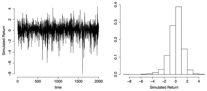
Simulated dataset from the SVML-GH-ST: Time series of returns (left) and the histogram (right).

We set the prior distributions as follows: β₀ ~ 𝒩(0, 100), β₁ ~ 𝒩_(−1,1)(0.1, 100), β₂ ~ 𝒩(−0.1, 100), α|τ² ~ 𝒩(0, τ²/0.002), ϕ|τ² ~ 𝒩_(−1,1)(0.95, 100), τ² ~ ℐ𝒢 (2.5, 0.025), φ|τ² ~ 𝒩(−0.3, τ²/0.005), δ ~ 𝒩(0, 1) and ν ~ 𝒢(12, 0.5). The prior means of β₁ and ϕ are, respectively, 0.0032 and 0.0003 and the corresponding prior variances are 0.3328 and 0.3329. In both cases, the priors are equivalent to the uniform distribution on interval (−1, 1), which gives zero mean and variance of 0.3333. Thus, it is clear that the priors specified for β₁ and ϕ are essentially non-informative.

The number of blocks, K, in the block sampler was set equal to 30 so that each block contained 66 $h_t^{\prime }s$ on average. We conducted the MCMC simulation for 50,000 iterations. The first 10,000 draws were discarded as a “burn-in” period, and then the next 40,000 were recorded. In order to reduce the autocorrelation between successive values of the simulated chain, only every 10th values of the chain were stored. With the resulting 4000, we calculated the posterior means, the 95% credible intervals and the convergence diagnostic (CD) statistics proposed by Geweke [16] for all the parameters.

The proposed algorithm is evaluated in terms of how well it estimates the true parameter values. From Table 1 and Figure 2, it can be seen that the estimated results for the parameters appear quite reasonable, because all the 95% credible intervals include true values. According to the CD values, the null hypothesis that the sequence of 4000 draws is stationary was accepted at the 5% level for all the parameters in all the models considered here. The inefficiency factor is defined by $1+{\sum }_{s=1}^{\infty }{\rho }_s$, where ρ_s is the sample auto-correlation at lag s. It measures how well the MCMC chain mixes [see, e.g, 23]. It is the estimated ratio of the numerical variance of the posterior sample mean to the variance of the sample mean from uncorrelated draws. When the inefficiency factor is equal to m, we need to draw MCMC samples m times as many as the number of uncorrelated samples. From Table 1, we found that our algorithm produces a good mixing of the MCMC chain. This fact is further confirmed in Figure 3, where the the autocorrelation function (acf) of the parameters shows a faster decay.

Table 1.

Simulated dataset: summary results for tge SVML-GH-ST model

Parmater	True value	Posterior mean	95% CI	IF	CD
β0	0.2500	0.2810	(0.1220, 0.4650)	6.26	−0.12
β1	0.0300	0.0260	(−0.0170, 0.0680)	1.28	0.95
β2	−0.2000	−0.2500	(−0.4450,−0.0700)	5.38	0.01
α	−0.0080	−0.0160	(−0.0340,−0.0030)	10.36	−0.95
ϕ	0.9500	0.9210	(0.8680, 0.9610)	10.67	−1.01
${\sigma }_{\eta }^2$	0.0225	0.0330	(0.0160, 0.0550)	21.83	0.96
δ	−0.5000	−0.7680	(−1.6100,−0.3400)	21.31	−0.32
ρ	0.3500	−0.2350	(−0.4270,−0.0420)	7.02	0.52
ν	10.0000	12.4430	(8.2330, 19.5520)	20.02	0.15

Figure 2.

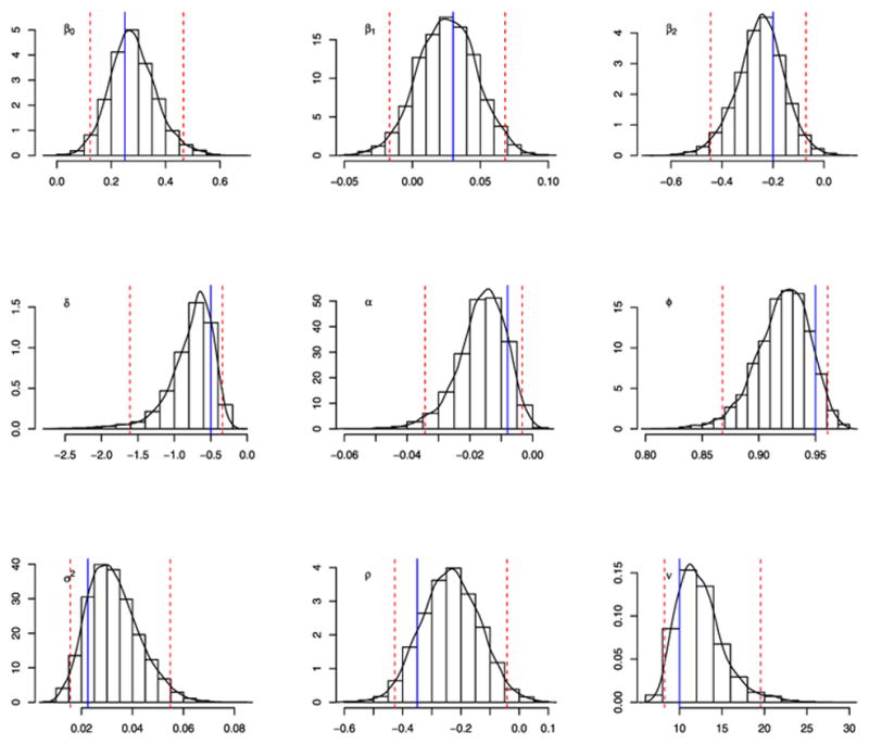
Simulated dataset. Histograms and estimated densities from the MCMC output for the SVML-GH-ST. The solid line indicates the true value and the dotted line the 95% credible interval.

Figure 3.

SVML-GH-ST, simulated dataset. Autocorrelation function (acf) for the parameters obtained from the MCMC output.

In Figure 4, the smoothed mean calculated from the MCMC output (dotted line) and true values (solid line) of ${\mathrm{e}}^{\frac{h_t}{2}}$ are shown. They show that the estimated values follow the behavior of the true volatilities.

Figure 4.

SVML-GH-ST, simulated dataset. True values (solid line) and posterior smoothed mean (dotted line) of $e^{\frac{h_t}{2}}$.

4. EMPIRICAL APPLICATION

This section analyzes the daily closing prices for the S&P 500 stock market index. The S&P 500 index contains the stocks of 500 Large-Cap corporations. Although a majority of those corporations are US based, it also includes other companies having their common stocks within the index. The data set was obtained from the Yahoo finance web site available to download at http://finance.yahoo.com. The period of analysis is January 4, 1980 – December 31, 2015, which yields 9078 observations. Throughout, we work with the compounded return expressed as y_t = 100(log P_t − log P_t−1), where P_t is the closing price on day t.

The compounded S&P 500 returns are plotted in Figure 5 as a time series and also as a histogram. The mean and standard deviation (SD) of returns are 0.03 and 1.12, respectively. As shown in Figure 5, the returns are skewed (−1.16) with heavy tails. From Table 2, we also note that the returns have a large range (minimum, −22.90 and maximum, 10.95). Some extreme observations, explained by some turbulences in financial markets as the stock market crash occurred by October 1987, the Asian financial crises in July 1997, the Russian financial crises in August 1998 and the U. S. market subprime crises in December 2007, contribute to the large kurtosis (29.54) of the S&P 500 returns. As a result, the S&P 500 index returns likely depart from the underlying normality assumption.

Figure 5.

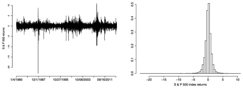
Compounded S & P 500 index returns from January 4, 1980 to December 31, 2015. The left panel shows the plot of the raw series and the right panel the histogram of returns.

Table 2.

Summary statistics for the S&P 500 returns

Median	SD	Minimum	Maximum	Skewness	Kurtosis
0.03	1.12	−22.90	10.95	−1.16	29.54

We fitted the SVML-N, SVML-T, and SVML-GH-ST models. In all cases, we simulated the h_t’s in a multi-move fashion with stochastic knots based on the method described in Section 2.2. We set the prior distributions for the common parameters as follows: β₀ ~ 𝒩(0, 100), β₁ ~ 𝒩_(−1,1)(0.1, 100), β₂ ~ 𝒩(−0.1, 100), ϕ ~ 𝒩_(−1,1)(0.95, 100), τ² ~ ℐ𝒢(2.5, 0.025), α | τ² ~ 𝒩(0, τ₂/0.002), and φ | τ² ~ 𝒩(−0.3, τ²/0.005). The prior distribution on the shape parameter was chosen as ν ~ 𝒢(12, 0.8) for the SVML-T and SVML-GH-ST models, respectively. For the SVML-GH-ST, we set δ ~ 𝒩(0, 100). The initial values of the parameters were randomly generated from the prior distributions. We set initial values of all the log-volatilities, h_t, to be zero. Finally the initial z_1:T were generated from the prior p(z_t | ν).

For the block sampler algorithm, we set the number of blocks K to be 180 in such a way that each block contained 50 $h_t^{\prime }\mathrm{s}$ on average. For the SVML-N, SVML-T, and SVML-GH-ST models, we conducted the MCMC simulation for 25,000 iterations. In all the cases, the first 5000 draws were discarded as a burn-in period. As before, in order to reduce the autocorrelation between successive values of the simulated chain, only every 10th values of the chain were stored. With the resulting 2000 values, we calculated the posterior means, the 95% credible intervals and the convergence diagnostic (CD) statistics [16]. Table 3 summarizes the results. According to the CD values, the null hypothesis that the sequence of 2000 draws is stationary was accepted at the 5% level for all the parameters in all the models considered here. From Table 3 and Figure 7, we found that our algorithm yields a good mixing of the MCMC chain.

Table 3.

Estimation results for the S & P 500 index returns. First row: Posterior mean. Second row: 95% credible interval in parentheses. Third row: CD statistics. Fourth row: Inefficiency factors

Parameter	SVML-N	SVML-T	SVML-GH-ST
	0.0614	0.1801	0.0608
β0	(0.0378,0.0863)	(0.0274,0.0761)	(0.0356,0.0867)
	1.78	−0.70	−0.77
	1.63	1.76	1.78
	0.0017	−0.0081	−0.0122
β1	(−0.0193,0.0231)	(−0.0271, 0.01226)	(−0.0316,0.0082)
	−0.01	1.08	−0.82
	1.00	1.00	1.00
	−0.0237	−0.0176	−0.0270
β2	(−0.0535,0.0058)	(−0.0446,0.0017)	(−0.0654, −0.0006)
	0.24	1.78	0.49
	1.54	1.25	1.26
	−0.0078	−0.0063	−0.0126
α	(−0.0125, −0.0037)	(−0.0102, −0.0030)	(−0.0184, −0.0074)
	−1.72	1.82	−1.46
	3.33	7.51	1.26
	0.9760	0.9787	0.9743
ϕ	(0.9679,0.9829)	(0.9643,0.9826)	(0.9661,0.9812)
	−1.84	1.17	0.68
	9.78	11.26	1.26
	0.0332	0.0243	0.0340
${\sigma }_{\eta }^2$	(0.0251,0.0431)	(0.0246,0.0918)	(0.0258,0.0437)
	1.51	−1.12	0.68
	17.30	26.33	13.40
	−0.3622	−0.5038	−0.2837
ρ	(−0.4385, −0.2904)	(−0.5933, −0.4145)	(−0.3443, −0.2192
	1.78	−1.69	−0.53
	5.25	11.00	2.36
	–	9.1988	10.7500
ν	–	(7.9690,16.9087)	(8.5897,13.7853)
	–	1.32	0.16
	–	26.25	46.83
	–	–	−0.1534
δ	–	–	(−0.3443, −0.2192)
	–	–	−0.53
	–	–	9.22

Figure 7.

S&P 500 returns dataset. Autocorrelation function (acf) for the parameters obtained from the MCMC output.

Table 3 shows that the posterior mean and 95% credible interval of ϕ. For all the models, the posterior means of ϕ are above 0.97, showing higher persistence, as expected. We found that the persistence values of the SVML-T and the SVML-GH-ST are slightly different from the one for the SVML-N. The posterior means of ${\sigma }_{\eta }^2$ under the SVML-N and SVML-GH-ST models are greater than the posterior mean under the SVML-T model, indicating that the volatilities of the SVML-T models is less variable than the equivalent SVML-N and SVM-GH-ST models.

The posterior means together with the 95% credible intervals of the three parameters, which govern the mean process for each of the three models, are reported in Table 3. In all cases the posterior mean of β₀ is always positive and statistically significant under each fitted model. The posterior mean of β₁ is positive for the SVML-N and negative for the SVML-T and SVML-GH-ST models and similar to the first-order autocorrelation (not reported here). Since the 95% credible interval contains zero, this coefficient is not significant. The β₂ parameter, which measures both the ex ante relationship between returns and volatility and the volatility feedback effect, has a negative posterior mean under all of the fitted models. Although the credible interval of β₂ barely contains zero under the SVML-N and SVML-T the models, its posterior distribution is primarily located in the negative range, as shown in Table 4. The posterior mean of β₂ in the SVML-GH-ST is negative and the 95% credibility interval does not contains zero. This result confirms previous results in the literature and indicates that when investors expect higher persistent levels of volatility in the future, they require compensation for this in the form of higher expected returns.

Table 4.

S & P 500 index returndataset: P(β₂ < 0) estimated from the MCMC output

	SVML-N	SVML-T.	SVML-GH-ST
P(β2 < 0)	0.9465	0.9710	0.9805

As expected for all the models considered here, the posterior means of ρ, the correlation coefficient between shocks to return at time t and shocks to volatility at time t + 1, are always negative and the 95% credible intervals do not contain zero. This result indicates that this parameter is statistically significant. Hence, we may conclude that there is a strong and significant “leverage effect” for the S & P 500 index returns returns dataset.

We found that the posterior mean of δ is −0.1534, which indicates that the returns are slightly asymmetric. We also found that the 95% credible interval does not contains zero.

The magnitude of the tail fatness is measured by the shape parameter ν in the SVML-T and SVML-GH-ST models. The posterior means of ν are almost 9.19 and 10.75 under the SVML-T and SVML-GH-ST models, respectively. This difference can be explained by δ, the extra asymmetry parameter, which is considered in the specification of the SVML-GH-ST model. These results seem to indicate that the measurement errors of the stock returns are better explained by heavy-tailed distributions.

Now, we compare the volatility estimates. In Figure 8, we plot the smoothed mean of ${\mathrm{e}}^{\frac{h_t}{2}}$. The posterior smoothed mean of ${\mathrm{e}}^{\frac{h_t}{2}}$ under the SVML-T, SVML-GH-ST models show smoother movements than that under the SVML-N model (solid line). Extreme returns, such as the stock market crash occurred and the U. S. market subprime crises in December 2007, clearly make the differences. The models with heavy tails accommodate possible outliers in a somewhat different way by inflating the variance ${\mathrm{e}}^{\frac{h_t}{2}}$ by $z_t^{\frac{1}{2}}{\mathrm{e}}^{\frac{h_t}{2}}$. This can have a substantial impact, for instance, on the evaluation of derivative instruments and several strategic or tactical asset allocation topics.

Figure 8.

S & P 500 returns dataset. Posterior smoothed mean (dotted line) of $e^{\frac{h_t}{2}}$, SVML-GH-ST (solid line), SVML-T (dotted line), SVML-N (tiny line).

To assess the goodness of the estimated models, we calculate the deviance information criteria, DIC [39], Bayesian predictive information criteria, BPIC [6, 7] and the log-predictive score, LPS [19, 18, 12, 5, 2]. The DIC is defined as

$$\text{DIC}=-2E_{\mathit{\theta }\mid {\mathbf{y}}_{1:T}}[logp({\mathbf{y}}_{1:T}\mid \mathit{\theta })]+p_D.$$ (12)

The second term in (12) measures the complexity of the model by the effective number of parameters, p_D, defined as the difference between the posterior mean of the deviance and the deviance evaluated at the posterior mean of the parameters:

$$p_D=2[logp({\mathbf{y}}_{1:T}\mid \overline{\mathit{\theta }})-E_{\mathit{\theta }\mid {\mathbf{y}}_{1:T}}[logp({\mathbf{y}}_{1:T}\mid \mathit{\theta })]].$$ (13)

To calculate the DIC in the context of SVML-GHST model, we use the conditional likelihood $p({\mathbf{y}}_{1:T}\mid \alpha ,\varphi ,{\sigma }_{\eta }^2,\nu ,\delta ,\rho ,{\beta }_0,{\beta }_1,{\beta }_2,{\mathbf{z}}_{1:T},{\mathbf{h}}_{0:T})$, in this case θ encompasses ${(\alpha ,\varphi ,{\sigma }_{\eta }^2,\nu ,\delta ,\rho ,{\beta }_0,{\beta }_1,{\beta }_2)}^{\prime }$, z_1:T and h_1:T.

As pointed by Stone [40], Robert and Titterington [34], Celeux et al. [9], and Ando [7], the DIC suffers from some theoretical aspects. First, in the derivation of DIC, Spiegelhalter et al. [39] assumed that the specified parametric family of probability distributions that generate future observations encompasses the true model. This assumption may not always hold true. Secondly, the observed data are used both to construct the posterior distribution and to compute the posterior mean of the expected log-likelihood. Thus, the bias in the estimate of DIC tends to underestimate the true bias considerably. To overcome these theoretical problems in DIC, recently Ando [7] proposed the Bayesian predictive information criterion (BPIC) as an improved alternative of the DIC. The BPIC criterion is defined as

$$\mathit{BPIC}=-2E_{\mathit{\theta }\mid {\mathbf{y}}_{1:T}}[log\{p({\mathbf{y}}_{1:T}\mid \mathit{\theta })\}]+2T\widehat{b},$$ (14)

where b̂ is given by

$$\stackrel{\sim }{b}\approx \frac{1}{T}\left\{E_{\mathit{\theta }\mid {\mathbf{y}}_{1:T}}[log\{p({\mathbf{y}}_{1:T}\mid \mathit{\theta })p(\mathit{\theta })\}]-log[p({\mathbf{y}}_{1:T}\mid \widehat{\mathit{\theta }})p(\widehat{\mathit{\theta }})]+\text{tr}\{J_T^{-1}(\widehat{\mathit{\theta }})I_T(\widehat{\mathit{\theta }})\}+0.5q\right\}.$$ (15)

Here q is the dimension of θ, E_θ|y1:T [.] denotes the expectation with respect to the posterior distribution, θ̂ is the posterior mode, and

$$\begin{gathered} I_T(\widehat{\mathit{\theta }})=\frac{1}{T}\sum _{t=1}^T{\left(\frac{\partial {\eta }_T(y_t,\mathit{\theta })}{\partial \mathit{\theta }}\frac{\partial {\eta }_T(y_t,\mathit{\theta })}{\partial {\mathit{\theta }}^{\prime }}\right)|}_{\mathit{\theta }=\widehat{\mathit{\theta }}}, \\ {J}_T(\widehat{\mathit{\theta }})=\frac{1}{T}\sum _{t=1}^T{\left(\frac{{\partial }^2{\eta }_T(y_t,\mathit{\theta })}{\partial \mathit{\theta }\partial {\mathit{\theta }}^{\prime }}\right)|}_{\mathit{\theta }=\widehat{\mathit{\theta }}}, \end{gathered}$$

with η_T (y_t, θ) = logp(y_t | y_1:t−1, θ) + log p(θ)/T.

Scoring rules provide summary measures for the evaluation of probabilistic forecast by assigning a numerical score based on the predictive distribution and on the event or value that materializes. The fit of the models studied here will be assessed using log predictive scores [19, 18, 12, 5, 2]. The average log predictive score for the one-step ahead prediction is given by

$$\text{LPS}=-\frac{1}{T}\sum _{t=1}^{T}logp(y_t\mid {\mathbf{y}}_{1:t-1},\widehat{\mathit{\theta }}),$$ (16)

where θ̂ is an estimate of the model parameters and p(y_t | y_1:t−1,θ̂ ) is the one-step ahead predictive density. The smaller the DIC, BPIC and LPS values, the better the model fits the data.

In the SVML class of models, the log-likelihood function, log p(y_1:T | θ) and p(y_t | y_1:t−1, θ) are estimated using the auxiliary particle filter [see, e.g., 33, 30] with 10,000 particles. Table 5 shows the values of BPIC. According with the DIC, BPIC and LPS criterion, the SVML-GH-ST model fits the data better among all the considered models, suggesting that the S&P 500 index returns return data demonstrate sufficient departure from underlying normality assumptions.

Table 5.

S&P 500 returns dataset. Deviance Information Criteria (DIC), Bayesian predictive information criteria (BPIC) and Log Predictive Score (LPS)

Modelo	DIC	Ranking	BPIC	Ranking	LPS	Ranking
SVML-N	23579.7	3	23988.9	3	1.321	3
SVML-T	23502.3	2	23957.5	2	1.320	2
SVML-GH-ST	23452.7	1	23941.8	1	1.318	1

In order to check the distribution assumptions of the SV models, we use an approach similar to Kim, Shephard and Chib [24]. The diagnostics test is based on the probability integral transform of the realizations $y_{t+1}^o$ taken with respect to the one-step-ahead prediction density p(y_t+1 | y_1:t, θ). The probability integral transform, ε_t+1, is simply the cumulative distribution function corresponding to the prediction density p(y_t+1 | y_1:t, θ) evaluated at $y_{t+1}^o:{\epsilon }_{t+1}=Pr(y_{t+1}\le y_{t+1}^o\mid {\mathbf{y}}_{1:t},\mathit{\theta })$. For t = 1, . . . , T, under the null hypothesis that the true distribution of $y_{t+1}^o$ is p(y_t+1 | y_1:t, θ) (or equivalently, the model is correctly specified), the ε_t+1 converges in distribution to independent and identically distributed uniform random variables on [0, 1] [see, 35, 38, 24, 15, 28, among others]. By letting ς_t+1 = Φ⁻¹(ε_t+1), where Φ() denotes the standard normal cumulative distribution function, a sequence of independent standard normal random variables ς_t+1 is obtained, which are the standardized innovations. The probability $Pr(y_{t+1}\le y_{t+1}^o\mid {\mathbf{y}}_{1:t},\mathit{\theta })$ can then be approximated by

$$Pr(y_{t+1}\le y_{t+1}^o\mid {\mathbf{y}}_{1:t},\mathit{\theta })=\frac{1}{n}\sum _{i=1}^{N}Pr(y_{t+1}\le y_{t+1}^o\mid {\mathbf{y}}_{1:t},h_{t+1}^{(i)},\mathit{\theta }).$$

The QQ-plots for pseudo residuals the three models fitted, SVML-N, SVML-T and SVML-GH-ST are shown in Figure 9. The qq-plots indicate a lack of fit in the left tail, specially in the SVML-N and SVML-ST models. The indicated mis-specification could be solved by using the SVML with generalized skew-Student-t or skew-Student-t distributions as in Abanto-Valle et al. [5] and Abanto-Valle et al. [2].

Figure 9.

S & P 500 returns dataset. Quantile-Quantile plot of the residuals ς_t. The solid line plots the quantiles of the 𝒩(0, 1) against the quantiles of the standard normal and the points were the sorted values of ς_t against the quantiles of the standard normal.

5. CONCLUSIONS

This article presented a Bayesian implementation of a robust alternative for estimation in the stochastic volatility-in-mean model with correlated errors, as an extension of the model proposed by [26] and Abanto-Valle et al. [3] via MCMC methods. The SVML model enables us to investigate the dynamic relationship between returns and their time-varying volatility. The Gaussian assumption of the mean innovation was replaced by univariate thick-tailed processes, known as the variance-mean mixture of the normal distribution. Under a Bayesian perspective, we developed an algorithm based on MCMC simulation methods to estimate all the parameters and latent quantities in our proposed SVML-GH-ST model. We illustrated our methods through an empirical application of the S&P 500 returns series, which shows that the SVML-GH-ST model provides a better fit than the SVML-N and SVML-T models in terms of parameter estimates, interpretation, and robustness aspects. The β₂ estimate, which measures both the ex ante relationship between returns and volatility and the volatility feedback effect, was found to be negative. These results are in line with those of French et al. [14], who found a similar relationship between unexpected volatility dynamics and returns, and confirm the hypothesis that investors require higher expected returns when unanticipated increases in future volatility are highly persistent. This is consistent with our findings of higher values of ϕ combined with larger negative values for the in-mean parameter. On the other hand, since the posterior mean and 95% credible interval contains only negative values, we can conclude that there is a strong and significant “leverage effect” for the S&P 500 returns dataset.

Our SVML-GH-ST models showed considerable flexibility to accommodate outliers, but their robustness aspects could be seriously affected by the prior of the ν and δ parameters. In this set-up, for example, it would be possible to study different objective priors for the parameters in the GH-ST distributions in the same spirit of the works of Fonseca et al. [13] and Salazar et al. [36] or using a different skew-student-t parameterization as in Abanto-Valle et al. [5] and [2] for example. Nevertheless, an in-depth investigation of this modification is beyond the scope of the present paper, but provides stimulating topics for future research.

Figure 6.

S&P 500 returns dataset. Histograms and estimated densities from the MCMC output for the SVML-GH-ST. The solid line indicates the posterior mean and the dotted line the 95% credible interval.

APPENDIX A: THE FULL CONDITIONAL DISTRIBUTIONS

In this appendix, we describe the full conditional distributions for the parameters and the mixing latent variables z_1:T of the SVML-GH-ST model.

Full conditional distributions of β₀, β₁, and β₂

Let m_t and V_t be defined by

$$\begin{gathered} m_t=\{\begin{array}{ll}\sqrt{z_t}{\mathrm{e}}^{\frac{h_t}{2}}\frac{\phi }{{\tau }^2+{\phi }^2}(h_{t+1}-\alpha -\varphi h_t),\hfill & t<T,\hfill \\ 0,\hfill & t=T,\hfill \end{array} \\ {V}_t=\{\begin{array}{ll}{z}_t{\mathrm{e}}^{h_t}\frac{{\tau }^2}{{\tau }^2+{\phi }^2},\hfill & t<T,\hfill \\ z_t{\mathrm{e}}^{h_t},\hfill & t=T.\hfill \end{array} \end{gathered}$$

For parameters β₀, β₁ and β₂, we set the prior distributions as: ${\beta }_0~\mathcal{N}({\overline{\beta }}_0,{\sigma }_{{\beta }_0}^2),{\beta }_1~{\mathcal{N}}_{(-1,1)}({\overline{\beta }}_1,{\sigma }_{{\beta }_1}^2),{\beta }_2~\mathcal{N}({\overline{\beta }}_2,{\sigma }_{{\beta }_2}^2)$. Then, the full conditionals are given by

$${\beta }_0\mid {\mathbf{y}}_{0:T},{\mathbf{h}}_{1:T},{\mathbf{z}}_{1:T},{\beta }_1,{\beta }_2~\mathcal{N}(\frac{b_{{\beta }_0}}{a_{{\beta }_0}},\frac{1}{a_{{\beta }_0}}),$$ (A.1)

$${\beta }_1\mid {\mathbf{y}}_{0:T},{\mathbf{h}}_{1:T},{\mathbf{z}}_{1:T},{\beta }_0,{\beta }_1~\mathcal{N}(\frac{b_{{\beta }_1}}{a_{{\beta }_1}},\frac{1}{a_{{\beta }_1}}){\mathbb{I}}_{\mid {\beta }_2\mid <1},$$ (A.2)

$${\beta }_2\mid {\mathbf{y}}_{0:T},{\mathbf{h}}_{1:T},{\mathbf{z}}_{1:T},{\beta }_0,{\beta }_1~\mathcal{N}(\frac{b_{{\beta }_2}}{a_{{\beta }_2}},\frac{1}{a_{{\beta }_2}}),$$ (A.3)

where $a_{{\beta }_0}={\sum }_{t=1}^T\frac{1}{V_t}+\frac{1}{{\sigma }_{{\beta }_0}^2},b_{{\beta }_0}={\sum }_{t=1}^T\frac{w_t}{V_t}+\frac{{\overline{\beta }}_0}{{\sigma }_{{\beta }_0}^2},a_{{\beta }_1}={\sum }_{t=1}^T\frac{y_{t-1}^2}{V_t}+\frac{1}{{\sigma }_{{\beta }_1}^2},b_{{\beta }_1}={\sum }_{t=1}^T\frac{u_t{y}_{t-1}}{V_t}+\frac{{\overline{\beta }}_1}{{\sigma }_{{\beta }_1}^2},a_{{\beta }_2}={\sum }_{t=1}^T\frac{{\mathrm{e}}^{2h_t}}{V_t}+\frac{1}{{\sigma }_{{\beta }_2}^2},b_{{\beta }_2}={\sum }_{t=1}^T\frac{r_i{\mathrm{e}}^{h_t}}{V_t}+\frac{{\overline{\beta }}_2}{{\sigma }_{{\beta }_2}^2},w_t=y_t-{\beta }_1{y}_{t-1}-{\beta }_2{\mathrm{e}}^{h_t}-{\mathrm{e}}^{\frac{h_t}{2}}\delta (z_t-{\mu }_z)-m_t,u_t=y_t-{\beta }_0-{\beta }_2{\mathrm{e}}^{h_t}-{\mathrm{e}}^{\frac{h_t}{2}}\delta (z_t-{\mu }_z)-m_t,r_t=y_t-{\beta }_0-{\beta }_1{y}_{t-1}-{\mathrm{e}}^{\frac{h_t}{2}}\delta (z_t-{\mu }_z)-m_t$, and 𝕀_|β2|<1 is the indicator variable.

Full conditional distributions of α, ϕ, φ, δ, and τ²

We assume the following prior distributions: α | τ² ~ 𝒩(α₀, τ²/q₀), φ | τ² ~ 𝒩(φ₀, τ²/p₀), $\varphi ~{\mathcal{N}}_{(-1,1)}({\varphi }_0,s_{\varphi }^2),\delta ~\mathcal{N}({\delta }_0,s_{\delta }^2)$, and τ² ~ 𝒢I(a_τ/2, S_τ /2), where α₀, φ₀, ϕ₀, $s_{\varphi }^2$, δ₀, $s_{\delta }^2$, a_τ, S_τ, p₀, and q₀ are known hyper parameters.

After some simple but tedious algebra, we obtain

$$\alpha \mid .~\mathcal{N}(\frac{B_{\alpha }}{A_{\alpha }},\frac{{\tau }^2}{A_{\alpha }}),$$ (A.4)

$$\phi \mid .~\mathcal{N}(\frac{B_{\phi }}{A_{\phi }},\frac{{\tau }^2}{A_{\phi }}),$$ (A.5)

$$\delta \mid .~\mathcal{N}(\frac{B_{\delta }}{A_{\delta }},\frac{1}{A_{\delta }}),$$ (A.6)

where $A_{\alpha }=q_0+\frac{1+\varphi }{1-\varphi }+T-1,B_{\alpha }={\alpha }_0{q}_0+(1+\varphi )h_1+{\sum }_{t=1}^{T-1}{k}_t,k_t=h_{t+1}-\varphi h_t-\phi g_t{z}_t^{-\frac{1}{2}}{\mathrm{e}}^{-\frac{h_t}{2}},A_{\phi }=p_0+{\sum }_{t=1}^{T-1}{g}_t^2{z_t}^{-1}{\mathrm{e}}^{-h_t},B_{\phi }={\phi }_0{p}_0+{\sum }_{t=1}^{T-1}{c}_t{g}_t{z}_t^{-\frac{1}{2}}{\mathrm{e}}^{-\frac{h_t}{2}},A_{\delta }=-\frac{\phi }{{\tau }^2}{\sum }_{t=1}^{T-1}\frac{1}{\sqrt{z_t}}(z_t-{\mu }_z)(h_{t+1}-\alpha -\varphi h_t)+\left(\frac{{\phi }^2+{\tau }^2}{{\tau }^2}\right){\sum }_{t=1}^{T-1}\frac{1}{z_t{e}^{h_t/2}}(z_t-{\mu }_z)(y_t-{\beta }_0-{\beta }_1{y}_{t-1}-{\beta }_2{e}^{h_t}),B_{\delta }=\left(\frac{{\phi }^2+{\tau }^2}{{\tau }^2}\right){\sum }_{t=1}^{T-1}\left(\frac{1}{z_t}{(z_t-{\mu }_z)}^2\right)+\frac{1}{z_n}{(z_n-{\mu }_z)}^2+\frac{1}{s_{\delta }^2}$, c_t = h_t+1 − α − ϕh_t, and $g_t=y_t-{\beta }_0-{\beta }_1{y}_{t-1}-{\beta }_2{\mathrm{e}}^{h_t}-{\mathrm{e}}^{\frac{h_t}{2}}\delta (z_t-{\mu }_z)$. In a similar way, the conditional distribution of ϕ is given by

$$p(\varphi \mid .)\propto Q(\varphi )exp\left\{-\frac{A_{\varphi }}{2}{\left(\varphi -\frac{B_{\varphi }}{A_{\varphi }}\right)}^2\right\},$$ (A.7)

where

$$Q(\varphi )=\sqrt{1-{\varphi }^2}exp\{-\frac{1-{\varphi }^2}{2{\tau }^2}{(h_1-\frac{\alpha }{1-\varphi })}^2\},$$

$A_{\varphi }=\frac{1}{s_{\varphi }^2}+{\sum }_{t=1}^{T-1}\frac{h_t^2}{{\tau }^2},B_{\varphi }=\frac{{\varphi }_0}{s_{\varphi }^2}+{\sum }_{t=1}^{T-1}\frac{l_t{h}_t}{{\tau }^2},l_t=h_{t+1}-\alpha -\phi (y_t-{\beta }_0-{\beta }_1{y}_{t-1}-{\beta }_2{\mathrm{e}}^{h_t})z_t^{-\frac{1}{2}}{\mathrm{e}}^{-\frac{h_t}{2}}$, and 𝕀_|ϕ|<1 is the indicator variable. As p(ϕ | h_1:T, α, $p(\varphi \mid {\mathbf{h}}_{1:T},\alpha ,{\sigma }_{\eta }^2)$) in (A.7) does not have a closed form, we sample from it by using the Metropolis-Hastings algorithm with truncated ${\mathcal{N}}_{(-1,1)}(\frac{b_{\varphi }}{a_{\varphi }},\frac{{\sigma }_{\eta }^2}{a_{\varphi }})$ as the proposal density. The conditional distribution of τ² is $\mathcal{I}\mathcal{G}(\frac{T_1}{2},\frac{M_1}{2})$, where T₁ = a_τ +T +2 and $M_1=(1-{\varphi }^2){(h_1-\frac{\alpha }{1-\varphi })}^2+{\sum }_{t=1}^{T-1}{(c_t-\phi z_t^{-\frac{1}{2}}{\mathrm{e}}^{-\frac{h_t}{2}}{g}_t)}^2+p_0{(\phi -{\phi }_0)}^2+q_0{(\alpha -{\alpha }_0)}^2+S_{\tau }$. Once τ² and φ are sampled, respectively, from their conditional posteriors, we can calculate ρ and ${\sigma }_{\eta }^2$ through ${\sigma }_{\eta }^2={\tau }^2+{\phi }^2$ and ρ = φ/σ_η.

Full conditional distributions of z_t and ν

The full conditional distribution of z_t is given by

$$p(z_t\mid .)\propto Q(z_t){\left(\frac{\gamma }{\vartheta }\right)}^{\lambda }\frac{z^{\lambda -1}}{2K_{\lambda }(\gamma ,\vartheta )}exp\{-\frac{1}{2}({\vartheta }^2{z}_t^{-1}+{\gamma }^2{z}_t)\},$$

where the values of λ, ϑ and γ are the parameters of a distribution GIG(λ, ϑ, γ) whose values are given by

$$\begin{gathered} \lambda =-\frac{\nu +1}{2}, \\ {\gamma }^2={\delta }^2\frac{{\phi }^2+{\tau }^2}{{\tau }^2}, \\ {\vartheta }^2=\frac{{\phi }^2+{\tau }^2}{{\tau }^2}{e}^{-h_t}\times {\left(y_t-{\beta }_0-{\beta }_1{y}_{t-1}-{\beta }_2{e}^{h_t}+{\mu }_z{e}^{h_t/2}\delta \right)}^2+\nu . \end{gathered}$$

We sample z_t by the Metropolis-Hastings algorithm. We use GIG(λ, ϑ, γ) as the proposal distribution such that $z_t^{\ast }$ and $z_t^{(i-1)}$ are the proposal value and previous iteration value, respectively. Thus, the acceptance probability is given by ${\alpha }_{MH}=min\{1,\frac{Q(z_t^{\ast })}{Q(z_t^{(i-1)})}\}$, where

$$Q(z_t)=exp\left\{\frac{\phi }{{\tau }^2}\right[z_t^{-1/2}{e}^{-h_t/2}(h_{t+1}-\alpha -\varphi h_t)\left(y_t-{\beta }_0-{\beta }_1{y}_{t-1}-{\beta }_2{e}^{h_t}+{\mu }_z{e}^{h_t/2}\delta \right)--z_t^{1/2}\delta (h_{t+1}-\alpha -\varphi h_t)\left]{\mathbb{I}}_{\{t<n\}}\right\}.$$

We assume the prior distribution of ν as 𝒢(a_ν, b_ν)𝕀_4<ν≤40. Then, the full conditional distribution of ν is

$$p(\nu \mid {\mathbf{z}}_{1:T})\propto \frac{{\frac{\nu }{2}}^{\frac{T\nu }{2}}}{\mathrm{\Gamma }{\left(\frac{\nu }{2}\right)}^T}exp\{-\sum _{t=1}^T\frac{1}{2V_t}[y_t-{\beta }_0-{\beta }_1{y}_{t-1}-{\beta }_2{\mathrm{e}}^{h_t}-{\mathrm{e}}^{\frac{h_t}{2}}\delta \left(z_t-\frac{\nu }{\nu -2}\right)-{m_t]}^2-\frac{\nu }{2}\sum _{t=1}^T\left[\frac{1}{z_t}+log{z}_t\right]\}{\nu }^{a_{\nu }-1}exp\{-b_{\nu }\nu \}{\mathbb{I}}_{4<\nu \le 40}.$$

We sample ν by the Metropolis-Hastings algorithm [43, 10]. Let ν* denote the mode (or approximate mode) of p(ν | z_1:T ), and let ℓ(ν) = logp(ν | z_1:T ). We use the proposal density ${\mathcal{N}}_{(4,40)}({\mu }_{\nu },{\sigma }_{\nu }^2)$, where μ_ν = ν* − ℓ′(ν*)/ℓ″(ν*) and ${\sigma }_{\nu }^2=-1/{\ell }^{″}({\nu }^{\ast })$. ℓ′(ν*) and ℓ″(ν*) are the first and second derivatives of ℓ(ν) evaluated at ν = ν*.

APPENDIX B: SOME DERIVATIONS OF THE BLOCK SAMPLER

First, we define

$$d_s=\frac{\partial L}{\partial h_s}=-\frac{1}{2}+\frac{{(y_s-{\mu }_s)}^2}{2V_s}+\frac{(y_s-{\mu }_s)}{V_s}\frac{\partial {\mu }_s}{\partial h_s}+\frac{(y_{s-1}-{\mu }_{s-1})}{V_{s-1}}\frac{\partial {\mu }_{s-1}}{\partial h_s}-\varphi \frac{(h_{s+1}-\alpha -\varphi h_s)}{{\sigma }_{\eta }^2}\mathbb{I}(t+k<T)$$ (B.1)

for s = t + 1, . . . , t + k, and

$$\mathbf{Q}=\left(\begin{array}{ccccc}{M}_{t+1}& N_{t+2}& 0& \dots & 0\\ N_{t+2}& M_{t+2}& N_{t+3}& \dots & 0\\ 0& N_{t+3}& M_{t+3}& \ddots & ⋮\\ ⋮& \ddots & \ddots & \ddots & N_{t+k}\\ 0& \dots & 0& N_{t+k}& M_{t+k}\end{array}\right),$$ (B.2)

where

$$M_s=-E\left[\frac{{\partial }^{2}L}{\partial h_s^2}\right]=\frac{1}{2}+\frac{1}{V_s}{\left(\frac{\partial {\mu }_s}{\partial h_s}\right)}^2+\frac{1}{V_{s-1}}{\left(\frac{\partial {\mu }_{s-1}}{\partial h_s}\right)}^2+\frac{{\varphi }^2}{{\sigma }_{\eta }^2}\mathbb{I}(t+k<T),s=t+1,\dots ,t+k,$$ (B.3)

$$N_s=-E\left[\frac{{\partial }^{2}L}{\partial h_s\partial h_{s-1}}\right]=\frac{1}{V_{s-1}}\frac{\partial {\mu }_{s-1}}{\partial h_{s-1}}\frac{\partial {\mu }_{s-1}}{\partial h_s},$$ (B.4)

where s = 2, . . . , T and N_t+1 = 0. Next, we define

$$\frac{\partial {\mu }_s}{\partial h_s}=\{\begin{array}{ll}{\beta }_2{e}^{h_s}+\frac{1}{2}{\mathrm{e}}^{\frac{h_s}{2}}\delta (z_s-{\mu }_z)+\frac{\phi }{{\phi }^2+{\tau }^2}\sqrt{z_s}{\mathrm{e}}^{\frac{h_s}{2}}\left[\frac{(h_{s+1}-\alpha -\varphi h_s)}{2}-\varphi \right]\hfill & s=1,\dots ,T-1,\hfill \\ {\beta }_2{\mathrm{e}}^{h_s}+\frac{1}{2}{\mathrm{e}}^{\frac{h_s}{2}}\delta (z_s-{\mu }_z),\hfill & s=T,\hfill \end{array}$$ (B.5)

$$\frac{\partial {\mu }_{s-1}}{\partial h_s}=\{\begin{array}{ll}0,\hfill & s=1,\hfill \\ \frac{\phi }{{\phi }^2+{\tau }^2}\sqrt{z_{s-1}}{\mathrm{e}}^{\frac{h_s-1}{2}},\hfill & s=2,\dots ,T.\hfill \end{array}$$ (B.6)

References

- 1.Abanto-Valle CA, Bandyopadhyay D, Lachos VH, Enriquez I. Robust Bayesian analysis of heavy-tailed stochastic volatility models using scale mixtures of normal distributions. Computational Statistics & Data Analysis. 2010;54:2883–2898. doi: 10.1016/j.csda.2009.06.011. [DOI] [PMC free article] [PubMed] [Google Scholar]
- 2.Abanto-Valle CA, Dey DK, Lachos VH. Bayesian estimation of a skew-Student-t stochastic volatility model. Methodology and Computing in Applied Probability. 2015;17:721–738. [Google Scholar]
- 3.Abanto-Valle CA, Migon HS, Lachos VH. Stochastic volatility in mean models with scale mixtures of normal distributions and correlated errors: A Bayesian approach. Journal of Statistical Planning and Inference. 2011;54:1875–1887. [Google Scholar]
- 4.Abanto-Valle CA, Migon HS, Lachos VH. Stochastic volatility in mean models with heavy-tailed distributions. Brazilian Journal of Probability and Statistics. 2012;26(4):402–422. [Google Scholar]
- 5.Abanto-Valle CA, Wang C, Wang X, Wang F-X, Chen M-H. Bayesian inference for stochastic volatility models using the generalized skew-t distribution with applications to the Shenzhen stock exchange return. Statistical and Its Interface. 2014;7:487–502. [Google Scholar]
- 6.Ando T. Bayesian inference for nonlinear and nongaussian stochastic volatility model with leverge effect. Journal of Japan Statistical Society. 2006;36:173–197. [Google Scholar]
- 7.Ando T. Bayesian predictive information criterion for the evaluation of hierarchical Bayesian and empirical Bayes models. Biometrika. 2007;94:443–458. [Google Scholar]
- 8.Bollerslev T, Zhou H. Volatility puzzles: A simple framework for gauging return-volatility regressions. Journal of Econometrics. 2005;131:123–150. [Google Scholar]
- 9.Celeux G, Forbes F, Robert CP, Titterington DM. Deviance information criteria for missing data models. Bayesian Analysis. 2006;1:651–674. [Google Scholar]
- 10.Chib S. Marginal likelihood from the Gibbs output. Journal of the American Statistical Association. 1995;90:1313–1321. [Google Scholar]
- 11.de Jong P, Shephard N. The simulation smoother for time series models. Biometrika. 1995;82:339–350. [Google Scholar]
- 12.Delatola E-I, Griffin JE. Bayesian nonparametric modelling of the return distribution with stochastic volatility. Bayesian Analysis. 2011;6:901–926. [Google Scholar]
- 13.Fonseca TCO, Ferreira MAR, Migon HS. Objective Bayesian analysis for the Student-t regression model. Biometrika. 2008;95:325–333. [Google Scholar]
- 14.French KR, Schert WG, Stambugh RF. Expected stock return and volatility. Journal of Financial Economics. 1987;19:3–29. [Google Scholar]
- 15.Gerlach R, Carter C, Kohn R. Diagnostics for time series analysis. Journal of Time Series Analysis. 1999;20:309–330. [Google Scholar]
- 16.Geweke J. Evaluating the accuracy of sampling-based approaches to the calculation of posterior moments. In: Bernardo JM, Berger JO, Dawid AP, Smith AFM, editors. Bayesian Statistics. Vol. 4. Oxford, U.K: Oxford University Press; 1992. pp. 169–193. [Google Scholar]
- 17.Ghysels E, Harvey AC, Renault E. Stochastic volatility. In: Maddala G, Rao CR, editors. Handbook of Statistics. Vol. 14. Amsterdam: North-Holland; 1996. pp. 119–191. [Google Scholar]
- 18.Gneiting T, Raftery AE. Strictly proper scoring rules, prediction and estimation. Journal of the American Statistical Association. 2007;6:901–926. [Google Scholar]
- 19.Good IJ. Rational decisions. Journal of the Royal Statistical Society, Series B. 1952;14:107–114. [Google Scholar]
- 20.Harvey AC, Shephard N. The estimation of an asymmetric stochastic volatility model for asset returns. Journal of Business and Economic Statistics. 1996;14:429–434. [Google Scholar]
- 21.Jacquier E, Polson N, Rossi P. Bayesian analysis of stochastic volatility models. Journal of Business and Economic Statistics. 1994;12:371–418. [Google Scholar]
- 22.Jacquier E, Polson N, Rossi P. Bayesian analysis of stochastic volatility models with fat-tails and correlated errors. Journal of Econometrics. 2004;122:185–212. [Google Scholar]
- 23.Kim S, Shepard N, Chib S. Stochastic volatility: Likelihood inference and comparison with ARCH models. Review of Economic Studies. 1998;65:361–393. [Google Scholar]
- 24.Kim S, Shephard N, Chib S. Stochastic volatility: Likelihood inference and comparison with ARCH models. Review of Economic Studies. 1998;65:361–393. [Google Scholar]
- 25.Koopman S. Disturbance smoothers for state space models. Biometrika. 1993;80:117–126. [Google Scholar]
- 26.Koopman SJ, Uspensky EH. The stochastic volatility in mean model: Empirical evidence from international tock markets. Journal of Applied Econometrics. 2002;17:667–689. [Google Scholar]
- 27.Liesenfeld R, Jung RC. Stochastic volatility models: Conditional normality versus heavy-tailed distrutions. Journal of Applied Econometics. 2000;15:137–160. [Google Scholar]
- 28.Liesenfeld R, Richard J-F. Univariate and multivariate stochastic volatility models: Estimation and diagnostics. Journal of Empirical Finance. 2003;10:505–531. [Google Scholar]
- 29.Nakajima J, Omori Y. Stochastic volatility model with leverage and asymmetrically heavy-tailed error using GH skew Student’s t-distribution. Computational Statistics & Data Analysis. 2012;56:3690–3704. [Google Scholar]
- 30.Omori Y, Chib S, Shephard N, Nakajima J. Stochastic volatility with leverage: Fast likelihood inference. Journal of Econometrics. 2007;140:425–449. [Google Scholar]
- 31.Omori Y, Watanabe T. Block sampler and posterior mode estimation for asymmetric stochastic volatility models. Computational Statistics & Data Analysis. 2008;52:2892–2910. [Google Scholar]
- 32.Pemstein D, Quinn KV, Martin AD. The scythe statistical library: An open source C++ library for statistical computation. Journal of Statistical Software. 2011;42:1–26. [Google Scholar]
- 33.Pitt M, Shephard N. Filtering via simulation: Auxiliary particle filter. Journal of the American Statistical Association. 1999;94:590–599. [Google Scholar]
- 34.Robert CP, Titterington DM. Discussion on “Bayesian measures of model complexity and fit”. Biometrical Journal. 2002;64:573–590. [Google Scholar]
- 35.Rosenblatt M. Remarks on a multivariate transformation. Annals of Mathematical Statistics. 1952;23:470–472. [Google Scholar]
- 36.Salazar E, Migon HS, Ferreira MAR. Technical report. Federal University of Rio de Janeiro, Departament of Statistics; 2009. Objective Bayesian analysis for exponential power regression models. [Google Scholar]
- 37.Shephard N, Pitt M. Likelihood analysis of non-Gaussian measurements time series. Biometrika. 1997;84:653–667. [Google Scholar]
- 38.Smith JQ. Diagnostic checks of non-standard time series models. Journal of Forecasting. 1985;4:283–291. [Google Scholar]
- 39.Spiegelhalter DJ, Best NG, Carlin BP, van der Linde A. Bayesian measures of model complexity and fit. Journal of the Royal Statistical Society, Series B. 2002;64:621–622. [Google Scholar]
- 40.Stone M. Discussion on “Bayesian measures of model complexity and fit”. Journal of the Royal Statistical Society, Series B. 2002;64:621. [Google Scholar]
- 41.Taylor S. Financial returns modelled by the product of two stochastic processes-a study of the daily sugar prices 1961–75. In: Anderson O, editor. Time Series Analysis: Theory and Practice. Vol. 1. Amsterdam: North-Holland; 1982. pp. 203–226. [Google Scholar]
- 42.Taylor S. Modeling Financial Time Series. Chichester: Wiley; 1986. [Google Scholar]
- 43.Tierney L. Markov chains for exploring posterior distributions (with discussion) Annal of Statistics. 1994;21:1701–1762. [Google Scholar]
- 44.Watanabe T, Omori Y. A multi-move sampler for estimate non-Gaussian time series model: Comments on Shepard and Pitt (1997) Biometrika. 2004;91:246–248. [Google Scholar]
- 45.Yu J. On leverage in stochastic volatility model. Journal of Econometrics. 2005;127:165–178. [Google Scholar]