

Abstract
Mixed-effects model is an efficient tool for analyzing longitudinal data. The random effects in a mixed-effects model can be used to capture the correlations among repeated measurements within a subject. Mixed effects model can be used to describe individual response profile as well as population response profile. In this manuscript, we apply mixed-effects models to the repeated measurements of cardiac function variables including heart rate, coronary flow, and left ventricle developed pressure (LVDP) in the isolated, Langendorff-perfused hearts of glutathione s-transferase P1/P2 (GSTP) gene knockout and wild-type mice. Cardiac function was measured before and during ischemia/reperfusion injury in these hearts. To describe the dynamics of each cardiac function variable during the entire experiment, we developed piecewise nonlinear mixed-effects models and a change point nonlinear mixed effect model. These models can be used to examine how cardiac function variables were altered by ischemia/reperfusion-induced injury and to compare the cardiac function variable between genetically engineered (null or transgenic) mice and wild-type mice. Hypothesis tests were constructed to evaluate the impact of deletion of GSTP gene for different cardiac function variables. These findings provide a new application for mixed-effects models in physiological and pharmacological studies of the isolated Langendorff-perfused heart.
Keywords: Mixed-effects model, Piecewise nonlinear mixed-effects model, Change point model, Cardiac function, Ischemia-reperfusion
1. Motivation
Myocardial ischemia/reperfusion (I/R) injury has resulted in significant morbidity and numerous studies have been carried out to discover endogenous mechanisms to protect the heart against I/R injury. Glutathione s-transferase P (GSTP) has been identified as an antioxidant cardiac enzyme that protects against I/R injury by catalyzing the removal of toxic lipid peroxidation products [1]. In an isolated heart, cardiac function is monitored over time and function is characterized by heart rate (i.e., the number of beats per minute (bpm)), coronary blood flow (mL/min), and left ventricle developed pressure (LVDP) (i.e., the difference of left ventricle systolic pressure and left ventricle diastolic pressure; mmHg). To examine whether GSTP gene protects against I/R injury, the isolated, Langendorff-perfused hearts from GSTP-null mice (KO) and wild type mice (WT) were exposed to 30 min of ischemia followed by 45 min of reperfusion [1]. The cardiac function variables (heart rate, coronary blood flow, and LVDP) were measured continuously including 5 min pre-ischemia, 30 min of ischemia, and 45 min of reperfusion. The data were summarized in 1 min intervals. Heart rate, coronary blood flow, and LVDP are shown, respectively, in Fig. 1 Panels A1–A3 for wild-type mice (n = 7) and in Fig. 1 Panels B1–B3 for GSTP-null mice (n = 6). Typically, the Student’s t-test is used to test whether two groups are the same at each time point [2] or a repeated measures analysis of variance (rANOVA) is applied to test whether there are group difference, time effect, and group by time interaction [3]. The number of repeated observations for each subject is 80, and thus, the t-test without multiplicity adjustment seems inappropriate. The rANOVA requires that all individuals have a complete balanced data and a fixed time schedule, and the rANOVA treat time points as different levels of a factor variable. Because each cardiac function variable was recorded in 80 min interval, and each cardiac function variable changes dramatically over the three treatment periods (i.e., pre-ischemia, ischemia, and reperfusion), the application of rANOVA was limited. Thus, a more flexible model, mixed-effects model, seems to be more appropriate. In the mixed-effects model time points are not necessary fixed, time is treated as a continuous variable, and all available data can be used in mixed-effects model provided that data are missing at random [4]. In a mixed-effects model, the correlation between repeated measurements is captured by random effects [3]. Moreover, mixed-effects models provide a more flexible covariance structure for non-constant within-subject correlation [5]. Several studies have suggested that a mixed-effects model is very useful in biomedical research and especially in analyzing complex data with multi-source variance [6]. In many longitudinal analyses, change is assumed to be linear but in numerous situations, the change is not uniform but rather faster during some periods and slower in others [7]. In these cases, nonlinear mixed-effects (NLME) models or piecewise polynomials are more appropriate than linear mixed-effects (LME) models to describe these nonlinear changes. However, nonlinear models incorporate characteristics of the data, such as asymptotes and monotonicity; the parameters in nonlinear models are often interpretable; and nonlinear models often provide more reliable predictions for the response variable outside the observed range of the data than, say, polynomial models would [8]. Thus, in this paper, we applied NLME models to investigate the dynamics of the cardiac function variables.
Fig. 1.
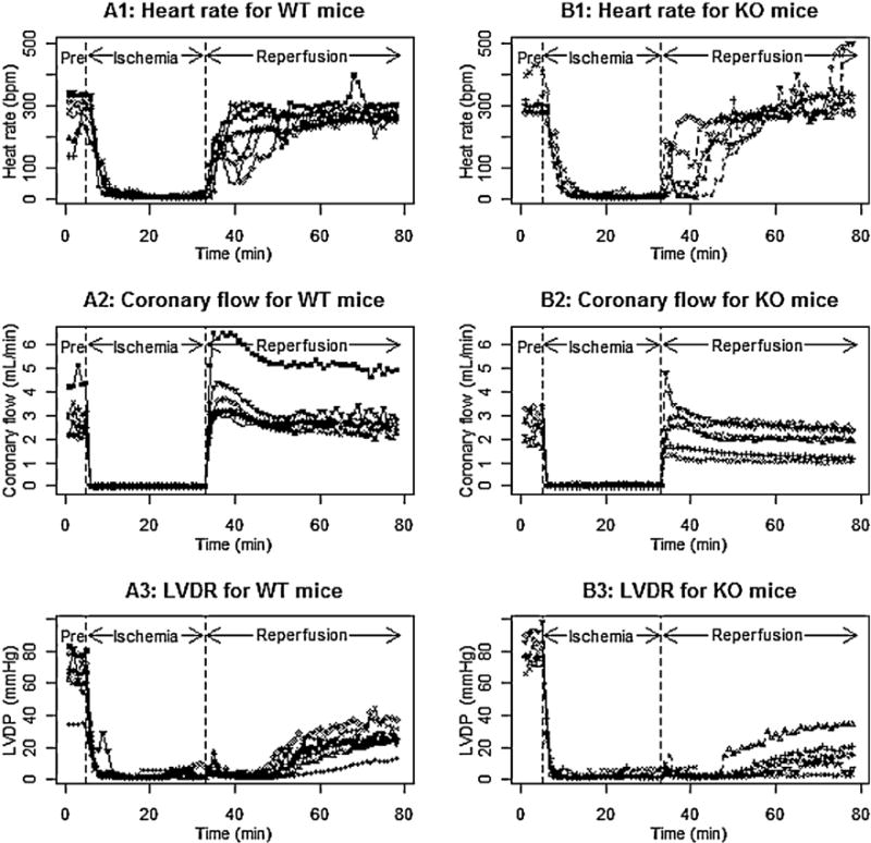
Individual profiles for heart rate (Panels A1 and B1), coronary flow (Panels A2 and B2), and left ventricle developed pressure (LVDP) (Panels A3 and B3) in WT mice and KO mice.
For hearts undergoing ischemia/reperfusion injury, cardiac function during pre-ischemia, ischemia, and reperfusion periods is quite different, and the change in function during each period is often nonlinear. To describe the heart rate and coronary blood flow for the entire experiment, we developed a nonlinear mixed model for each period and a piecewise nonlinear mixed model over the entire experiment. LVDP, the difference between left ventricle systolic pressure and left ventricle diastolic pressure, is an important variable to characterize cardiac function, and LVDP decreased to very low values during ischemia, and gradually increased during reperfusion. The elapsed time before there is an increase in the LVDP is inversely related to cardiac recovery, and a shorter elapsed time indicates a less injured heart. The comparison of LVDP between pre-ischemia and the recovery during reperfusion is not our interest. Therefore we only focus on modeling LVDP during reperfusion. The elapsed time from a constant phase to an increasing phase is often called a change point. Note that the elapsed times will differ for different subjects, and thus, we proposed a random change point nonlinear mixed-effects model for studying LVDP during reperfusion. In both the nonlinear mixed effect models or change point nonlinear mixed effects models, the parameters for each subject are expressed as the summation of group level parameters (i.e., fixed effects) and the deviation of the subject parameters away from its group level parameters (i.e., random effects). In Section 2.1, we provide a brief introduction to nonlinear mixed effect models, including parameter estimation and statistical inferences. In Section 2.2, we provide a general framework for change point mixed effect model. In Section 3, we develop nonlinear mixed effect models for examining heart rate and coronary blood flow, and the change point nonlinear mixed effects models for examining LVDP. In Section 4, we present the analytic results for the experiment data shown in Fig. 1. In Section 5, we carried out simulations to examine the performance of the estimation of parameters when the number of subjects is small and moderate. The last section provides relevant discussion of models and their potential applications.
2. General nonlinear mixed effect models and change point model
2.1. General nonlinear mixed-effects (NLME) model
NLME models are often used because these models provide a parsimonious description of the data and reliable predictions for the response variables [8]. The general formula of a single level NLME model is proposed by Lindstrom and Bates [5]. At the first level the jth observation on the ith subject is modeled as:
| (1) |
where i = 1,…,N, j = 1,…,ni, and εij ∼ N(0,σ). N is the number of subjects, ni is the number of observations on the ith subject, f is a real-valued function of a subject-specific parameter vector ϕi and a covariate vector tij, and εij is a normally distributed within-subject error term. The function f is nonlinear in at least one component of the subject-specific parameter vector ϕi, which is modeled as:
| (2) |
where β is a p-dimensional vector of fixed effects parameters, bi is a q-dimensional random effects vector associated with ith subject, and the matrices Ai and Bi are of appropriate dimensions and depend on the ith subject and possibly on the values of some covariates. Let us denote , and bi = (bi1,…,biq)T. It is generally assumed that (i) εi has normal distribution with mean zero and variance σ2I, (ii) bi has a normal distribution with mean zero and variance–covariance matrix D, and (iii) εi and bi are independent (i = 1,…,N) [8]. Here we assume that subjects’ responses follow a similar function form with parameters varying among subjects. The parameters for ith subject are the vector ϕi, which composite the fixed effect parameter β and random effects bi. The response function determined by fixed effect may be considered the average response for the population, and the response function determined by ϕi may be considered the response function for ith subject. The diagonal entries of the variance–covariance matrix D, say ,…, , reflect the variation of the random effects, indicating the between-subject variation. The off-diagonal entries, such as ρkk′ρkρk′, describes the covariance between bik and bik′, where ρkk′ is the correlation coefficient between bik and bik′. The matrix D could be specified as different forms, such as positive definite matrix, compound symmetric matrix, or a blocked diagonal matrix [3,8]. Let us denote θ as the parameters specifying D, that is, θ includes all parameters which capture ,… and ρkk, (1 ≤ k < k′ ≤ q). The θ specifying D and σ2 specifying the within-subject error are often called variance-covariance component parameters. The estimation of the fixed effect parameter β and the variance–covariance component parameters θ and σ2 can be obtained by maximizing the marginal distribution for y, which generally does not have a closed-form expression. To obtain the solutions for maximizing the marginal distributions, different approximations have been proposed. The nlme package in R (http://www.r-project.org/) is implemented by taking a first-order Taylor expansion of the model function f around the expected value of the random effects [5,8]. The nlme function in this package provides the estimates for β and the variance–covariance component parameters θ and σ2, the asymptotic variance for , and the 95% confidence intervals for all parameters. In addition, the predicted values for can also be obtained. Subsequently, one can obtain the response profile at the population level as and at the subject-level as for ith subject, and their variances by using the δ-method [9,10]. The statistical inferences for the estimable function of β could be carried out by using the Wald’s statistics or the likelihood ratio tests (LRT) [8,9]. We started with a full model that included all parameters and D as a blocked diagonal matrix. To obtain a parsimonious model, we first removed the least significant variance-covariance components, and then removed the least significant fixed effects parameter. The LRT and the Akaike Information Criterion (AIC) [11] were applied to obtain a parsimonious model for interpretation and statistical inferences.
2.2. Change point nonlinear mixed effect model
The change point nonlinear mixed effect model still has the general form (1), that is, yij = f(ϕi,xij) + εij, with εij ∼ N(0,σ2). However, the response variable for ith individual often includes K different phases. The first phase can be described as f1(ϕi1, t) for t ≤ γi1, the kth (k = 2,…,K − 1) phase could be described as fk(ϕik, t) for γik−1 < t ≤ γik, and the Kth phase could be described as fK(ϕiK, t) for t > γiK−1. Here γik (k = 1,…,K − 1) are often called the change point for ith subject from kth phase to (k + 1)th phase. When K = 2, the expected response profile can be expressed as:
| (3) |
Generally, we assume that the response profile is continuous at the change point γi, that is, f1(ϕi1, γi) = f2(ϕi2, γi). The individual response parameters (i.e., ϕi = (ϕi1, ϕi2, γi)) are expressed by the summation of fixed effects and random effects: ϕi = Aiβ + Bibi, as shown in Eq. (2). Cudeck and Klebe [12] illustrated the application of change point models to psychology, and implemented the algorithm in SAS. Pearson et al. [13] used a smoothing function in the change point model to smooth the response function at the change point. In this manuscript, we assume that the response function is continuous at the change point, and used the nlme package in R to obtain the estimates for the involved parameters. Model selection, parameter estimation, and statistical inferences follow the same principle as in the nonlinear mixed effect models mentioned in the previous section.
3. Piecewise nonlinear mixed effect models and change point model for cardiac function variables
In this section, we applied exponential growth function of the form y = A(1 − e−kt) (where t > 0 and k > 0) [8] to describe the dynamics of heart rate and LVDP during reperfusion, and applied exponential decaying function of the form y = Ae−kt) (where t > 0 and k > 0) to describe the heart rate during ischemia We applied the first-order compartment model along with the exponential growth function to describe the coronary flow during reperfusion [8,13]. The parameters in these models incorporate theoretical characteristics of the data and are often easy to interpret.
3.1. Piecewise nonlinear mixed-effects model for heart rate
As illustrated in Fig. 1 (Panels A1, B1), heart rate does not change significantly during pre-ischemia in either WT mice or KO mice, declines exponentially during ischemia, and then increases gradually reaching a stable plateau during reperfusion. We propose using a constant (say ϕi1) to describe the heart rate in pre-ischemia, an exponential decaying function of the form ϕi1exp(−exp(ϕi2)(t − 5)+) to describe the heart rate during ischemia, and exponential growth function of the form ϕi3[1 − exp(−exp(ϕi4)(t − 35)+)] to describe the heart rate during reperfusion. The step function x+ is defined as x if x > 0, and zero otherwise. The step functions (t − 5)+ and (t − 35)+, respectively, are the time since the start of ischemia and the time since the start of reperfusion. The heart rate for ith subject during the entire experiment can be described as:
| (4) |
The parameter for ith subject, say ϕi = (ϕi1, ϕi2, ϕi3, ϕi4), depends on its group assignment (i.e., WT or KO mice) as well as the deviation from group-level parameters. That is,
| (5) |
and
| (6) |
Model (4) implies that the function is continuous during the entire experimental period. For example, the heart rate during pre-ischemia is ϕi1, and the heart rate at the beginning of ischemia is also ϕi1 since ϕi1exp(−exp(ϕi2)(t − 5)+) goes to ϕi1 when t goes to 5 from right. The heart rate declines to zero during ischemia, and recovers during reperfusion and tends to stabilize at a value ϕi3 during the later phase of reperfusion. The exp(ϕi2) is the decline rate constant during ischemia, and exp(ϕi4) is the increasing rate constant during reperfusion. The group-level response profile for WT mice is characterized by the parameters βk1 (k = 1,…,4), and obtained by replacing ϕik with βk1 (k = 1,…,4) in Eq. (4). The group-level response profile for KO mice is characterized by the parameters βk1 + βk2 (k = 1,…,4), and obtained by replacing ϕik with βk1 + βk2 (k = 1,…,4) in Eq. (4). The response profile for ith subject is characterized by the summation of its group-level parameter, i.e., βk1 + βk2typei (fixed effects), and the deviation from its group-level parameter, i.e., bik (k = 1,…,4) (random effects). The difference between WT and KO can be characterized by βk2 (k = 1,…,4). In addition, β11 and β11 + β12, respectively, describe the average heart rate for KO and WT hearts in pre-ischemia, and β31 and β31 + β32, respectively, describe the stabilized heart rate during reperfusion for WT and KO mice. It is straight forward to test whether the heart rate during reperfusion is recovered to pre-ischemia level for WT and KO mice, respectively, by testing β31 − β11 = 0 or (β31 + β32) − (β11 + β12) = 0.
3.2. Piecewise nonlinear mixed-effects model for coronary flow
Fig. 1 (Panels B1, B2) illustrates that coronary flow is close to a constant for WT mice and KO mice during pre-ischemia (say, ϕi1), drops to zero during ischemia, increases to a high peak shortly after the start of reperfusion, and then decreases gradually and plateaus at ϕi2 during reperfusion. To describe the coronary flow for WT mice and KO mice during the entire experiment, we propose the following piecewise nonlinear mixed-effects model:
| (7) |
where g(ϕi, t) = (ϕi5exp(ϕi3)/exp(ϕi4) − exp(ϕi3))[exp(− exp(ϕi3) (t − 35)+) − exp(− exp(ϕi4)(t − 35)+)], and ϕi = (ϕi1, ϕi2, ϕi3, ϕi4, ϕi5), and ϕik = βk1 + βk2 typei + bik (k = 1,…, 5) as shown in Eq. (5). The expression describing the coronary flow during reperfusion consists two components: the first component is an exponential growth curve with asymptote at ϕi2, while the second component, say g(ϕi, t), is a first-order compartment model, capturing the bell-shaped curves for the coronary flow [8,14]. In Eq. (7), the fixed effects β11 and β11 + β12 are, respectively, the means of the coronary flows for WT mice and KO mice in pre-ischemia; β21 and β21 + β22 represent, respectively, the stabilized coronary flow for WT mice and KO mice during reperfusion. The random effects bik (i = 1,…,N) describe the deviation of coronary flow for ith subject away from its group-level parameters. Using the parameters specified in the model, we can directly examine whether coronary flow for WT mice and KO mice during each time period is different by examining whether βk2 is different from zero. In addition, using the current specification, we can examine whether coronary flow during reperfusion recovers to its pre-ischemia level by testing if β21 − β11 = 0 for WT mice and testing if (β21 + β22) − (β11 + β12) = 0 for KO mice.
3.3. Change point nonlinear mixed effect models for left ventricle developed pressure (LVDP)
Fig. 1 (Panels A3, B3) illustrates that the LVDP is constant in pre-ischemia, decreases to a low value during ischemia, stays at the low value until an onset of increasing phase of LVDP during reperfusion, increases gradually after onset to plateau in the later stage of reperfusion. The onset values and the stabilized values were different for different subjects. We introduced random effects for the onset values and the stabilized values. The onset value and the stabilized LVDP were critically important because these characterized how quickly and to what degree the LVDP recovered. In consideration of all these aspects, we proposed the following change point model to describe the LVDP during reperfusion:
| (8) |
where ϕi = (ϕi1, ϕi2, ϕi3, ϕi4), and ϕik = βk1 + βk2 typei + bik (k = 1,…, 4). In model (8), ϕi1 is a constant LVDP before the onset of the increasing phase for LVDP, ϕi2 is the onset point (i.e., change point) from constant phase to the exponential growth phase, representing the unknown transition time between the constant LVDP and the exponential growth, ϕi1 + ϕi3 is the stabilized status of the LVDP during reperfusion, and exp(ϕi4) is the constant growth rate during the exponential LVDP growth phase. The subject-level parameters ϕik (k = 1,…, 4) are expressed as the summation of population parameters (i.e., βk1 + βk2 typei) and the deviation of the subject-level parameters away from their population parameters (i.e., bik). The population parameters are used to compare group differences, and the subject-level parameters are used to examine subject-level responses and between-subjects variations.
4. R-code and analysis results for cardiac function variables
We applied the proposed models to analyze the experimental data shown in Fig. 1. For each cardiac function variable, we started by fitting the full model, as proposed in Section 3, and we fitted several reduced models as well. The likelihood ratio tests (LRT) are applied to compare two nested models, and the LRT along with the AIC criterion are used to select a parsimonious model as our final model. We first consider a simplified variance–covariance matrix by setting the insignificant components from the full model to zero. If the LRT for comparing the reduced model and full model was not significant, we considered a further reduced model which excluded least significant fixed effects parameters. Otherwise, we remained the variance–covariance parameters in the model and considered a reduced model on the fixed effects parameters. The estimated parameters and their 95% confidence intervals in the full model, the reduced variance–covariance components model, and the final model are reported in Tables 1–3 for different cardiac function variables, and the interpretation and inferences for each cardiac function variable are based on the final parsimonious models. The fitted subject-level and group-level response curves are, respectively, shown in Panels A and B in Figs. 2–4, where the pointwise 95% confidence intervals for subject-level response curve and group-level response curves, along with the observations, are also shown. The Wald test was applied to test whether the cardiac function during reperfusion recovered to its pre-ischemia level. The nlme and anova in the R-package “nlme” are the major functions to be used for the analyses. The data frame for each cardiac function variable includes type (i.e., WT or KO), subject (i.e., subject identification number), time (in minutes), cardiac function variable, and period (i.e., pre-ischemia, ischemia, and reperfusion). The main results and the key R-code for each cardiac function variable is presented under the following sections.
Table 1.
Estimates of the parameters (Est.) and their 95% confidence intervals (95% CI) for modeling heart rate resulted from the full model, reduced model, and final model.
| Parameter | Full model
|
Reduced variance component model
|
Final model
|
|||
|---|---|---|---|---|---|---|
| Est. | (95% CI) | Est. | (95% CI) | Est. | (95% CI) | |
| β11 | 289.72 | (254.73, 324.71) | 289.73 | (254.77, 324.69) | 301.94 | (275.36, 328.51) |
| β12 | 26.45 | (−25.07, 77.97) | 26.44 | (−25.03, 77.91) | ||
| β21 | −1.11 | (−1.45, −0.77) | −1.11 | (−1.45, −0.77) | −1.01 | (−1.26, −0.75) |
| β22 | 0.22 | (−0.28, 0.72) | 0.22 | (−0.29, 0.72) | ||
| β31 | 276.54 | (193.43, 359.66) | 276.54 | (193.44, 359.65) | 276.54 | (193.36, 359.73) |
| β32 | 172.09 | (40.59, 303.59) | 172.10 | (40.62, 303.58) | 172.05 | (40.44, 303.65) |
| β41 | −1.65 | (−2.34, −0.96) | −1.65 | (−2.34, −0.96) | −1.65 | (−2.34, −0.96) |
| β42 | −1.32 | (−2.34, −0.30) | −1.32 | (−2.34, −0.30) | −1.32 | (−2.34, −0.3) |
| σl | 44.92 | (29.41, 68.63) | 44.88 | (29.37, 68.57) | 46.64 | (30.61, 71.06) |
| σ2 | 0.43 | (0.27, 0.71) | 0.44 | (0.27, 0.72) | 0.44 | (0.27, 0.72) |
| σ3 | 111.61 | (63.25, 196.93) | 111.59 | (61.42, 202.70) | 111.70 | (59.88, 208.38) |
| σ4 | 0.92 | (0.64, 1.33) | 0.92 | (0.60, 1.42) | 0.92 | (0.56, 1.5) |
| ρ12 | 0.02 | (−0.22, 0.26) | ||||
| ρ34 | −0.77 | (−0.91, −0.45) | −0.77 | (−0.92, −0.42) | −0.77 | (−0.93, −0.39) |
| σ | 33.40 | (31.95, 34.92) | 33.40 | (31.95, 34.92) | 33.41 | (31.95, 34.93) |
| AIC | 10,450.04 | 10,448.04 | 10,445.73 | |||
Table 3.
Estimates of the parameters (Est.) and their 95% confidence intervals (95% CI) for modeling left ventricle developed pressure (LVDP) during reperfusion based on full model and final model.
| Parameter | Full model
|
Final model
|
||
|---|---|---|---|---|
| Est. | (95% CI) | Est. | (95% CI) | |
| β11 | 3.22 | (2.53, 3.90) | 3.14 | (2.64, 3.64) |
| β12 | −0.15 | (−1.15, 0.86) | ||
| β21 | 51.60 | (49.30, 53.89) | 51.80 | (50.06, 53.53) |
| β22 | 0.50 | (−3.05, 4.04) | ||
| β31 | 25.26 | (18.75, 31.77) | 24.94 | (19.05, 30.82) |
| β32 | −10.50 | (−20.13, −0.88) | −9.96 | (−17.17, −2.75) |
| β41 | −2.38 | (−2.61, −2.16) | −2.40 | (−2.61, −2.19) |
| β42 | −0.30 | (−0.71, 0.11) | −0.27 | (−0.63, 0.09) |
| σ1 | 0.80 | (0.48, 1.33) | 0.79 | (0.47, 1.33) |
| σ2 | 3.02 | (1.91, 4.78) | 3.02 | (1.96, 4.66) |
| σ3 | 8.58 | (5.74, 12.82) | 8.74 | (5.87, 13.02) |
| σ4 | 0.24 | (0.08, 0.71) | 0.23 | (0.08, 0.67) |
| ρ12 | −0.62 | (−0.92, 0.18) | −0.66 | (−0.93, 0.10) |
| ρ13 | 0.18 | (−0.46, 0.70) | 0.18 | (−0.44, 0.68) |
| ρ14 | 0.48 | (−0.52, 0.92) | 0.47 | (−0.52, 0.92) |
| ρ23 | −0.70 | (−0.93, −0.11) | −0.68 | (−0.92, −0.11) |
| ρ24 | −0.60 | (−0.98, 0.74) | −0.67 | (−0.97, 0.41) |
| ρ34 | 0.08 | (−0.89, 0.92) | 0.13 | (−0.70, 0.81) |
| σ | 1.84 | (1.74, 1.96) | 1.85 | (1.74, 1.96) |
| AIC | 2540.96 | 2538.73 | ||
Fig. 2.
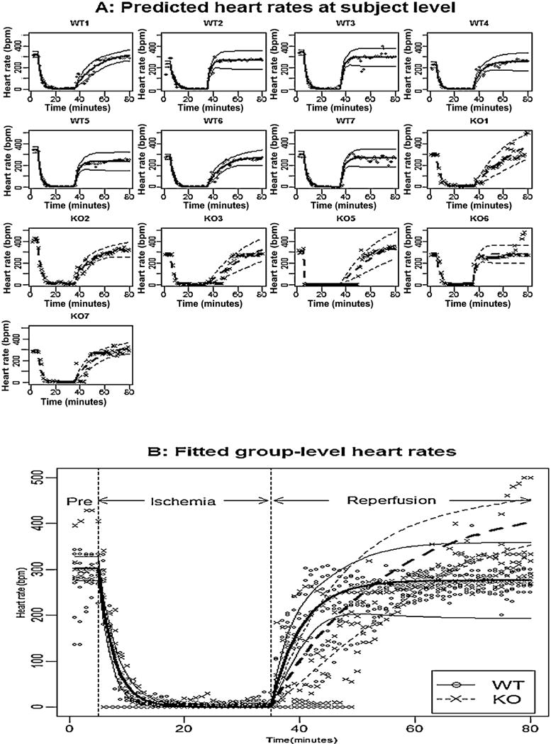
Panel A shows the observed heart rate for each mouse, the fitted subject-level heart rates, and their pointwise 95% confidence intervals; Panel B shows the observed heart rates for all mice, the fitted group-level heart rates, and their pointwise 95% confidence intervals for WT mice (solid line) and KO mice (dashed line).
Fig. 4.
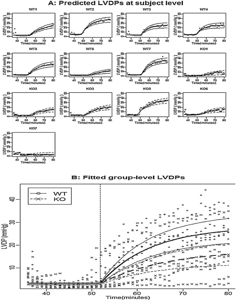
Panel A shows the observed LVDP for each mouse, the fitted subject-level LVDP, and their pointwise 95% confidence intervals; Panel B shows the observed LVDP for all mice, the fitted group-level LVDP, and their pointwise 95% confidence intervals for WT mice (solid line) and KO mice (dashed line).
4.1. Analysis results for heart rate
We started from the full model (4) with a block diagonal variance–covariance matrix for random effects bi, and the estimated parameters and their 95% confidence intervals are reported in Table 1 under the column title “Full model”. Since the correlation coefficients between bi1 and bi2 (i.e., ρ12) was not significantly different from zero, we fitted a reduced model with ρ12 being zero, and the fitted results are reported in Table 1 under the column title “Reduced variance component model”. The LRT for this reduced model versus the full model was not significant (p-value = 0.932). In the reduced model, the fixed effects parameters β12 and β22 were not significantly different from zero, we further removed these two parameters, and the LRT indicated that the final resulting model was not significantly different from the full model (p-value = 0.639) as well as the reduced variance component model (p-value = 0.431). The estimated parameters and their 95% confidence intervals for this model are reported in Table 1 under the column title “Final Model”. The observations, the fitted subject-level and group-level response curves based on the final model, along with their point-wise 95% confidence intervals, were shown in Fig. 2 Panel A and B, respectively. Based on the estimated parameters (Table 1 under the column title “Final model”) and the fitted values (Fig. 2), we conclude that: (i) in pre-ischemia, the heart rates of WT mice and KO mice were not significantly different because β12 was not significantly different from zero, and the between subject variation counts 66% of total variation since ; (ii) during reperfusion, the average stabilized heart rate for KO mice was significantly higher than that of WT mice because β32 was significantly larger than zero, and the between-subject variation was large and accounts for approximately 92% of the total variation; (iii) during reperfusion, the increasing rate constant for KO mice was significantly smaller than for WT mice because β42 was significantly smaller than zero; (v) during reperfusion, the subject-level stabilized heart rate was negatively associated with the increasing rate constant because the correlation between bi3 and bi4 (i.e., ρ34) was significantly smaller than zero. The R-code for analyzing heart rate is shown as follows:
HeartRate < -function(time,phi1,phi2,phi3,phi4){phi1*(time<= 5)+phi1*exp(-exp(phi2)*(time-5))*(time>5&time<=35)+as.numeric(SSasympOrig((time-35),
Asym=phi3,lrc=phi4))*(time>35)}
HR.full.nlme <-nlme(Rate∼HeartRate(time, phi1, phi2, phi3, phi4), na.action = na.omit,
fixed=phi1+phi2+phi3+phi4∼type,
random=pdBlocked(list(pdSymm(phi1+phi2∼1),pdSymm(phi3+phi4∼1))),
start=c(phi1=257.12,20,phi2=n1start[2],0.1,phi3=n2start[1],200,phi4= n2start[2],1), data=pre.isch.per,method=“ML”)
One can fit the reduced variance component model by replacing the “random” statement with “random = pdBlocked(list(pdDiag(phi1 + phi2 ∼ 1), pdSymm(phi3 + phi4 ∼ 1)))”, and fit the final model by additionally replacing the “fixed” statement with “fixed = list(phi1 + phi2 ∼ 1, phi3 + phi4 ∼ type)”.
We constructed test statistics to show if heart rate during reperfusion recovered to the pre-ischemic level for WT mice and KO mice. The associated null hypothesis for WT mice was H0: β11 − β31 = 0, and the associated null hypothesis for KO mice was H0: β11 − (β31 + β32) = 0. Based on the final model, the Wald test statistic for WT mice was ith a p-value at 0.568, indicating that the heart rate in pre-ischemia was not significantly different from the stabilized heart rate during reperfusion. The Wald test statistic for KO mice was with a p-value at 0.006, indicating that the heart rate in pre-ischemic is significantly lower than the stabilized heart rate during reperfusion.
4.2. Analysis of coronary flow
To examine coronary flow, we started from the full model (7) with a blocked diagonal matrix for random effects bi. The estimated parameters and their 95% confidence intervals for the full model are reported in Table 2 under the column title “Full model”. From the results of the full model, all the correlation coefficients except the one between bi2 and bi5 (i.e., ρ25) were not significantly different from zero. We fitted a reduced model with these variance components being zero, and the results are presented in Table 2 under the column “Reduced variance component model”. The AIC for the reduced model was smaller than the full model, and the LRT indicated that the two models were not significantly different (p-value = 0.07). Thus, the reduced model was preferred. Furthermore, we removed the least significant terms of fixed effects parameters. The LRT indicated that this model was not significantly different from the full model as well as the reduced variance component model. The results of the final model are reported in Table 2 under the column title “Final model”. The fitted subject-level coronary flow and group-level coronary flow are, respectively, shown in Panel A and B (Fig. 3), along with their pointwise 95% confidence intervals and the observed coronary flow. Based on the estimated parameters (Table 2) and the fitted values (Fig. 3), we conclude that (i) in pre-ischemia, the coronary flow between WT mice and KO mice was not significantly different because β12 was not significantly different from zero, and the between-subject variation accounted for 97.8% of the total variation; (ii) during reperfusion, the average stabilized coronary flow for WT mice was significantly higher than in KO hearts because β22 was significantly less than zero, and the between-subject variation was large and accounted for approximately 97.5% of the total variation. The R-code for analyzing coronary flow is shown as follows:
flow.pd<-function(phi1,phi2,phi3,phi4,phi5,time){phi1*(time<=5)+(phi2-phi2*exp(−exp(phi4)*(time-35))+phi5*exp(phi3)/(exp(phi4)-exp(phi3))*(exp(-exp(phi3)*(time-35))-exp(-exp(phi4)*(time-35))))*(time>=35)}
flow.full.nlme<-nlme(Flow∼flow.pd(phi1,phi2,phi3,phi4,phi5,time),
fixed=phi1+phi2+phi3+phi4+phi5∼type,
random=pdBlocked(list(phi1∼1, pdSymm(phi2+phi3+phi4+phi5∼1))),
start=c(phi1=2.86,−0.28,phi2=2.92,−1.03,phi3=0.03,0.69,phi4=−1.76,−0.3,phi5=4.15,−1.51),
data=td,method=“ML”)
Table 2.
Estimates of the parameters (Est.) and their 95% confidence intervals (95% CI) for modeling coronary flow resulted from the full model, reduced model, and final model.
| Parameter | Full model
|
Reduced variance component model
|
Final model
|
|||
|---|---|---|---|---|---|---|
| Est. | (95% CI) | Est. | (95% CI) | Est. | (95% CI) | |
| β11 | 2.86 | (2.37, 3.35) | 2.86 | (2.37, 3.35) | 2.73 | (2.38, 3.10) |
| β12 | −0.28 | (−1.00, 0.44) | −0.28 | (−0.99, 0.44) | ||
| β21 | 2.92 | (2.34, 3.51) | 2.92 | (2.35, 3.49) | 2.92 | (2.35, 3.49) |
| β22 | −1.03 | (−1.9, −0.17) | −1.02 | (−1.86, −0.19) | −1.02 | (−1.86, −0.18) |
| β31 | −0.10 | (−0.37, 0.33) | 0.01 | (−0.52, 0.53) | −0.01 | (−0.47, −1.50) |
| β32 | 0.72 | (−0.11, 0.94) | 0.81 | (−0.03, 1.64) | 0.71 (−0.05, 1.48) | |
| β41 | −1.89 | (−2.20, −1.20) | −1.70 | (−2.12, −1.27) | −1.77 | (−2.08, −1.47) |
| β42 | −0.19 | (−1.14, 0.40) | −0.00 | (−0.66, 0.67) | ||
| β51 | 4.12 | (3.18, 5.17) | 4.18 | (3.30, 5.06) | 4.18 | (3.29, 5.06) |
| β52 | −1.52 | (−2.92, −0.01) | −1.56 | (−2.85, −0.27) | −1.50 | (−2.80, −0.20) |
| σ1 | 0.66 | (0.44, 0.98) | 0.65 | (0.44, 0.97) | 0.67 | (0.44, 0.96) |
| σ2 | 0.77 | (0.51, 1.15) | 0.69 | (0.45, 1.05) | 0.63 | (0.51, 1.11) |
| σ3 | 0.70 | (0.46, 1.07) | 0.52 | (0.34, 0.80) | 0.47 | (0.29, 0.55) |
| σ4 | 0.54 | (0.35, 0.83) | 0.77 | (0.52, 1.14) | 0.77 | (0.26, 0.60) |
| σ5 | 1.17 | (0.78, 1.77) | 1.17 | (0.79, 1.74) | 1.18 | (0.83, 1.89) |
| ρ23 | 0.19 | (−0.35, 0.63) | ||||
| ρ24 | −0.17 | (−0.59, 0.32) | ||||
| ρ25 | 0.85 | (0.59, 0.95) | 0.85 (0.60, 0.95) | 0.84 (0.57, 0.95) | ||
| ρ34 | −0.44 | (−0.80, 0.16) | ||||
| ρ35 | 0.24 | (−0.29, 0.66) | ||||
| ρ45 | −0.02 | (−0.48, 0.44) | ||||
| σ | 0.10 | (0.10,0.11) | 0.10 | (0.10, 0.11) | 0.10 (0.10, 0.11) | |
| AIC | −1440.10 | −1460.48 | −1461.07 | |||
Fig. 3.
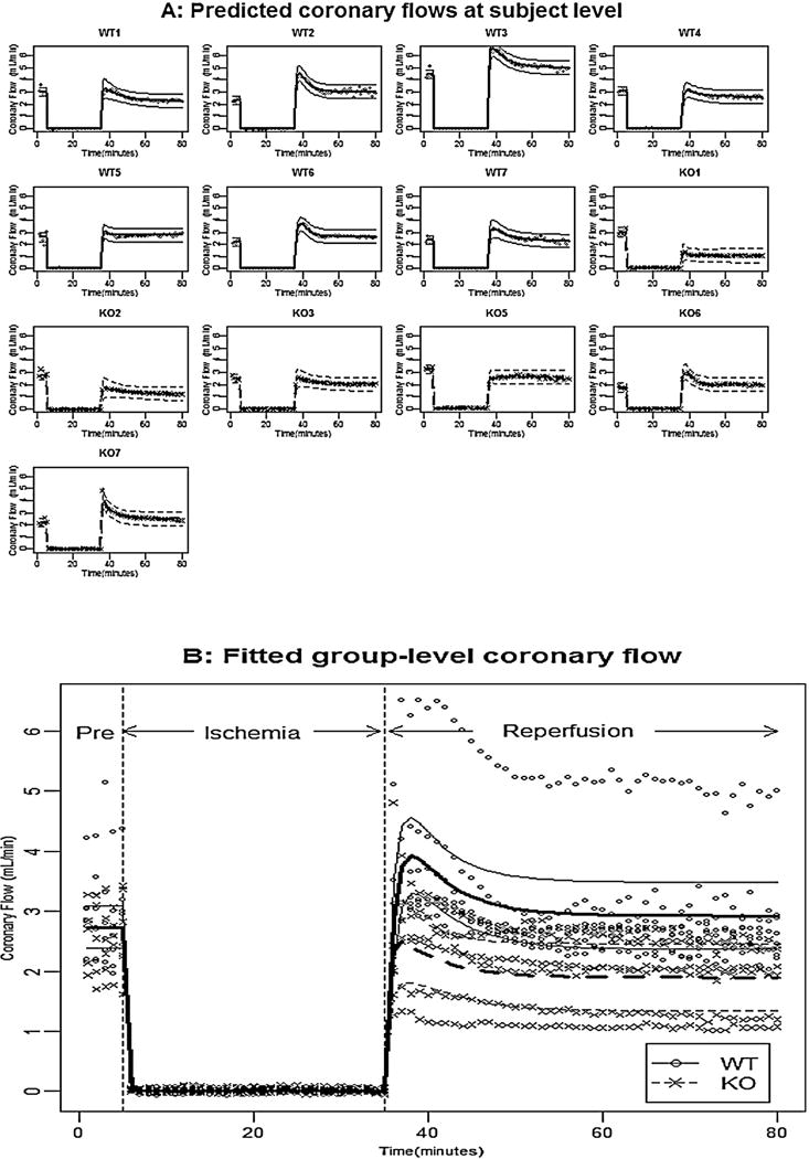
Panel A shows the observed coronary flow for each mouse, the fitted subject-level coronary flow, and their pointwise 95% confidence intervals; Panel B shows the observed coronary flow for all mice, the fitted group-level coronary flow, and their pointwise 95% confidence intervals for WT mice (solid line) and KO mice (dashed line).
One can fit the reduced variance component model by replacing the “random” statement with “random = pdBlocked(list(pdDiag(phi1 + phi3 + phi4 ∼ 1), pdSymm(phi2 + phi5 ∼ 1)))”, and fit the final model by additionally replacing the “fixed” statement with “fixed = list(phi1 + phi4 ∼ 1, phi2 + phi3 + phi5 ∼ type)”.
To test whether coronary flow during reperfusion recovered to the pre-ischemic level in WT and KO hearts, the Wald test statistic for WT mice was with a p-value at 0.57, indicating that the pre-ischemic coronary flow and the stabilized coronary flow during reperfusion were not significantly different. In the other word, the coronary flow during reperfusion recovered to pre-ischemic level in WT hearts. The Wald test statistic for KO mice was with a p-value at 0.02, indicating that the pre-ischemic coronary flow for KO mice was significantly higher than the stabilized coronary flow during reperfusion at significant level 0.05.
4.3. Analyses of LVDP
The change point nonlinear mixed-effects model (8) was applied to fit LVDP during-reperfusion observations, and the estimated parameters and their 95% confidence intervals are given in Table 3 under the column “Full model”. We fitted a reduced model excluding some non-significant variance components, however, the LRT for comparing the reduced model and the full model indicated that the two models were significantly different (p-value = 0.011). Therefore, we retained all variance components in the model. Notice that there were several insignificant fixed-effects parameters, we fitted a model without β12 and β22, and the LRT indicated that this model was not significantly different from the full model (p-value = 0.411). The results for this model are reported in Table 3 under the column title “Final model”. Based on the final model, the predicted subject-level LVDP and its pointwise 95% CI for each individual are presented in Fig. 4A, and the fitted group-level LVDP profile and their pointwise 95% CI for each group were shown in Fig. 4B. Based on the estimation of the parameters (Table 3) and fitted values (Fig. 4), we concluded that: (i) the LVDP before onset for WT mice and KO mice were not significantly different, and the between-subject variation was relative small as σ1 was relatively small; (ii) the change points for WT mice and KO mice were not significantly different, however, the between-subject variation was relative large as σ2 was relatively large; (iii) the stabilized LVDP for WT mice was significantly larger than that for KO mice because β32 was significantly less than zero; (iv) the increasing rate constant for WT mice was slightly larger than that for KO mice as β42 was slightly less than zero, although not significantly (p-value = 0.157). The R-code for analyzing LVDP is shown as follows:
t.pd<-function(phi1,phi2,phi3,phi4,time){phi1*(time<= phi2)+(phi1+phi3*(1-exp(-exp(phi4)*(time-phi2))))*(time>= phi2)}
lvdp.full.nlme<-nlme(DEVELOPED∼t.pd(phi1,phi2,phi3, phi4,time),
fixed=phi1+phi2+phi3+phi4∼type, random=phi1+phi2+phi3+phi4∼1,
start=c(phi1=n1start[1],0,phi2=n1start[2],0,phi3=n1start[3],0,phi4=n1start[4],0),
data=td,method=“ML”)
The final model can be obtained with replacing the “fixed” statement by “fixed=list(phi1+phi2∼1,phi3+phi4∼type)”. The detailed R-code and data sets can be obtained from the corresponding author.
5. Simulation study
In this paper, we applied the proposed models to analyzing an experimental data with a small sample size: 7 WT mice and 6 GSTP-KO mice, where there were 80 observations for each mouse. To examine the performance of the proposed models when the sample size is small or moderate, we carried out simulations under two scenarios: one scenario has a small sample size (say 7 WT mice and 6 GSTP-KO mice), and the other scenario has a moderate sample size (50 WT mice and 50 GSTP-KO mice). Under each scenario and for each cardiac function variable, we chose the final model in Section 4 as the underlying model to generate 1000 simulated data. Each simulated data was generated as follows: we first generated the random effect bi from N(0, D), where D, the covariance of bi, was specified by the variance–covariance component parameters in the final model; then we generated the subject-level parameters ϕik as βk1 + βk2 typei + bik, and subsequently, we generated the subject-level response profile as f(ϕi, t); the observations were generated by the subject-level response profile plus random sample from N(0, σ2). We fitted each simulated data set to the final model, the summarized statistics for the 1000 estimated parameters (e.g., mean, variance, and the mean squares for errors (MSE) under each scenario) were, respectively, reported in Tables 4–6 for heart rate, coronary flow, and LVDP. The MSE for each parameter was calculated as the summation of the variance and the squared difference between the sample mean and the underlying parameter. Based on the simulation results, we conclude that (1) the mean based on the 1000 simulated data under both scenarios are close to the underlying values, indicating that overall the estimates were not biased; (2) as the sample size goes from small to moderate, the variance and MSE dramatically decreased, indicating that the power of test statistics would increase as the sample size goes large.
Table 4.
Simulation results based on the final model for heart rate and 1000 simulated data sets.
| Parameter | True value |
nWT = 7 & nGSTP = 6
|
nWT = 50 & nGSTP = 50
|
||||
|---|---|---|---|---|---|---|---|
| Mean | Variance | MSE | Mean | Variance | MSE | ||
| β11 | 301.9 | 302.2 | 175.4 | 175.5 | 302.2 | 24.65 | 24.76 |
| β21 | −1.01 | −1.02 | 0.02 | 0.02 | −1.02 | <0.01 | <0.01 |
| β31 | 276.5 | 275.3 | 1674.8 | 1676.4 | 275.7 | 251.5 | 252.3 |
| β32 | 172.0 | 166.2 | 4456.5 | 4490.5 | 170.7 | 542.3 | 544.0 |
| β41 | −1.65 | −1.67 | 0.11 | 0.11 | −1.67 | 0.02 | 0.02 |
| β42 | −1.32 | −1.29 | 0.25 | 0.25 | −1.29 | 0.03 | 0.04 |
Table 6.
Simulation results based on the final model for LVDP and 1000 simulated data sets.
| Parameter | True value |
nWT = 7 & nGTSP = 6
|
nWT = 50 & nGTSP = 50
|
||||
|---|---|---|---|---|---|---|---|
| Mean | Variance | MSE | Mean | Variance | MSE | ||
| β11 | 3.14 | 3.20 | 0.05 | 0.05 | 3.14 | 0.01 | 0.01 |
| β21 | 51.80 | 51.22 | 0.44 | 0.76 | 51.83 | 0.10 | 0.10 |
| β31 | 24.94 | 24.89 | 6.60 | 6.60 | 24.85 | 1.13 | 1.14 |
| β32 | −9.96 | −10.43 | 12.69 | 12.91 | −9.96 | 1.41 | 1.41 |
| β41 | −2.40 | −2.47 | 0.01 | 0.02 | −2.40 | <0.01 | <0.01 |
| β42 | −0.27 | −0.26 | 0.02 | 0.02 | −0.27 | <0.01 | <0.01 |
6. Conclusion and discussion
In this study, we applied the mixed-effects models to the repeated measurements of cardiac function variables including heart rate, coronary flow, and left ventricle developed pressure in the isolated, Langendorff-perfused hearts of male glutathione s-transferase (GSTP1/P2) deficient (KO) mice [15] and WT (C57BL/6) mice. These particular mice were used because GSTP is a known antioxidant enzyme but its role as well as other GSTs in cardioprotection is unclear [16]. For this, we developed piecewise nonlinear mixed-effects models and change point model to describe the different cardiac function variables during the entire experiment. We examined how cardiac function variables are altered by ischemia/reperfusion challenge in KO mice and WT mice using nonlinear mixed-effects model and change point model. The Wald test and Akaike Information Criterion (AIC) are applied to obtain a parsimonious model for each cardiac function variable. The goodness of fit is examined, and the proposed models fit the experimental data very well. Moreover, nonlinear mixed-effects models provide not only interpretable models for the experimental data but also reliable predictions for the response variables in our experimental data. However, the models we developed in this paper are empirical models. In the future, some mechanism-based models may be worth investigating. Particularly, the model developed for coronary flow included four parameters capturing the bell-shaped response profiles. Some simplified mechanism-based model with less number of parameters will be a great interest. In this paper, we applied the models to the experimental data which included only 7 WT mice and 6 GSTP KO mice. When the sample size is small, the variances of the estimated parameters are usually large, and the power of the tests will be low. How to carry out power and sample size analyses is our great interest to work on. However, it is beyond the scope of this paper. Nevertheless, we have demonstrated that nonlinear mixed-effects models can be applied to the assessment of the cardiac function dynamics and the assessment of the treatment effect on the cardiac function. This work provides evidence of a new application for mixed-effects models in physiological and pharmacological studies of the isolated heart.
Table 5.
Simulation results based on the final model for coronary flow and 1000 simulated data sets.
| Parameter | True value |
nWT = 7 & nGSTP = 6
|
nWT = 50 & nGSTP = 50
|
||||
|---|---|---|---|---|---|---|---|
| Mean | Variance | MSE | Mean | Variance | MSE | ||
| β11 | 2.73 | 2.73 | 0.03 | 0.03 | 2.73 | 0.01 | 0.01 |
| β21 | 2.92 | 2.91 | 0.08 | 0.08 | 2.92 | 0.01 | 0.01 |
| β22 | −1.02 | −1.01 | 0.18 | 0.18 | −1.02 | 0.01 | 0.01 |
| β31 | 0.01 | 0.06 | 0.02 | 0.03 | 0.01 | 0.01 | 0.01 |
| β32 | 0.71 | 0.64 | 0.11 | 0.12 | 0.71 | 0.01 | 0.01 |
| β41 | −1.77 | −1.75 | 0.02 | 0.04 | −1.77 | 0.01 | 0.01 |
| β51 | 4.18 | 4.03 | 0.19 | 0.21 | 4.18 | 0.04 | 0.04 |
| β52 | −1.50 | −1.47 | 0.42 | 0.43 | −1.50 | 0.04 | 0.04 |
Acknowledgments
The study was supported by P20RR024489 (MK, DJC), U24HL094373 (MK), and HL89380 and HL89380-S10 (DJC). We thank L. Guo, M.D., for excellent technical assistance. We also thank the two reviewers and the Associate Editor for their constructive comments, which have helped to improve the paper significantly.
Footnotes
Conflict of interest statement
All authors in this manuscript do not have any conflicts of interest.
References
- 1.Conklin DJ, Hill BG, Kaiserova K, Guo Y, Bolli R, Bhatnagar A. Deficiency of glutathione s-transferase P (GSTP) mediated detoxification of lipid peroxidation products increases myocardial ischemia-reperfusion injury. Circulation. 2008;118:546–547. [Google Scholar]
- 2.West MB, Rokosh G, Obal D, Velayutham M, et al. Cardiac myocyte–specific expression of inducible nitric oxide synthase protects against ischemia/reperfusion injury by preventing mitochondrial permeability transition. Circulation. 2008;118:1970–1978. doi: 10.1161/CIRCULATIONAHA.108.791533. [DOI] [PMC free article] [PubMed] [Google Scholar]
- 3.Hedeker D, Gibbons RD. Longitudinal Data Analysis. John Wiley & Sons; New Jersey: 2006. [Google Scholar]
- 4.Krueger C, Tian L. A comparison of the general linear mixed model and repeated measures ANOVA using a dataset with multiple missing data points. Biological Research For Nursing. 2004;6:151–157. doi: 10.1177/1099800404267682. [DOI] [PubMed] [Google Scholar]
- 5.Lindstrom MJ, Bates DM. Nonlinear mixed effects models for repeated measures data. Biometrics. 1990;46:673–687. [PubMed] [Google Scholar]
- 6.Brown H, Prescott R. Applied Mixed Models in Medicine. John Wiley & Sons; New York: 1999. [Google Scholar]
- 7.Cudeck R, Harring JR. Analysis of nonlinear patterns of change with random coefficient models. Annual Review of Psychology. 2007;58:615–637. doi: 10.1146/annurev.psych.58.110405.085520. [DOI] [PubMed] [Google Scholar]
- 8.Pinheiro C, Bates DM. Mixed-Effects Models in S and S-PLUS. Springer-Verlag; New York: 2000. [Google Scholar]
- 9.Lehmann EL. Testing Statistical Hypotheses. 2nd. Wiley; New York: 1986. [Google Scholar]
- 10.Vonesh EF, Chinchilli VM. Linear and Nonlinear Models for the Analysis of Repeated Measurements. Marcel Dekker Inc.; New York, NY: 1997. [Google Scholar]
- 11.Akaike H. A new look at statistical model identification. IEEET Transactions on Automatic Control. 1974;19:716–722. [Google Scholar]
- 12.Cudeck R, Klebe KJ. Multiphase mixed-effects models for repeated measures data. Psychological Methods. 2002;7:41–63. doi: 10.1037/1082-989x.7.1.41. [DOI] [PubMed] [Google Scholar]
- 13.Pearson PD, Morrell CH, Landis PK, Carter HB, Brant LJ. Mixed-effects regression models for studying the natural history of prostate disease. Statistics in Medicine. 1994;13:587–601. doi: 10.1002/sim.4780130520. [DOI] [PubMed] [Google Scholar]
- 14.Hedaya A. Basic Pharmacokinetics. CRC Press; Boca Raton: 2007. [Google Scholar]
- 15.Henderson CJ, Smith A, Ure AGJ, Brown K, Bacon EJ, Wolf CR. Increased skin tumorigenesis in mice lacking pi class glutathione s-transferases. Proceedings of National Academy of Sciences. 1998;95:5275–5280. doi: 10.1073/pnas.95.9.5275. [DOI] [PMC free article] [PubMed] [Google Scholar]
- 16.Conklin DJ, Bhatnagar A. Are glutathione s-transferase null genotypes “null and void” of risk for ischemic vascular disease? Circulations: Cardiovascular Genetics. 2011;4:339–341. doi: 10.1161/CIRCGENETICS.111.960526. [DOI] [PMC free article] [PubMed] [Google Scholar]