Analysis of Clustered Competing Risks Data using Subdistribution Hazard Models with Multivariate Frailties

Abstract

Competing risks data often exist within a center in multicenter randomized clinical trials where the treatment effects or baseline risks may vary among centers. In this paper we propose a subdistribution hazard regression model with multivariate frailty to investigate heterogeneity in treatment effects among centers from multicenter clinical trials. For inference, we develop a hierarchical likelihood (or h-likelihood) method, which obviates the need for an intractable integration over the frailty terms. We show that the profile likelihood function derived from the h-likelihood is identical to the partial likelihood, and hence it can be extended to the weighted partial likelihood for the subdistribution hazard frailty models. The proposed method is illustrated with a dataset from a multicenter clinical trial on breast cancer as well as with a simulation study. We also demonstrate how to present heterogeneity in treatment effects among centers by using a confidence interval for the frailty for each individual center and how to perform a statistical test for such heterogeneity using a restricted h-likelihood.

1 Introduction

Competing risks (CR) data arise when an occurrence of an event precludes other type of events from being observed.¹ Two broad classes of models for analyzing the CR data have been developed based on Cox’s proportional hazards (PH) models; one is to model the cause-specific hazard of the different event types² and the other is to model the subhazard (i.e. the hazard function of a subdistribution) for the event of interest³. In particular, the subhazard model by Fine and Gray³, often referred to as the Fine-Gray model, directly associates covariate effects with the cumulative probability of a specific cause of events over time, i.e. the cumulative incidence function (CIF), whereas the cause-specific hazard model associates the covariate effects with the cause-specific hazard function. Therefore, if one is interested in direct statistical inference on the cumulative probability of cause-specific events, Fine-Gray model would be more appropriate.

In this paper we model the subhazard for the CR data from multi-center randomized clinical trials, which are often observed within a cluster (e.g. center). In many applications involving CR data, individual events within a cluster may be correlated due to unobserved shared factors across individuals. The Fine-Gray model, however, takes no account for such correlation, which can be modelled by the frailty (or random effect)^4,5. Thus Katsahian et al.⁶ and Christian⁷ have extended the Fine-Gray model to a subhazard frailty model with a random center effect only. It would be practically more useful to model heterogeneity in treatment effect among centers as well as the random center effect, where the two random effects might be correlated.^8,9 Here the heterogeneity in treatment effect among centers can be modelled as an additive frailty term to a regression coefficient for the baseline treatment effect without heterogeneity.¹⁰ In this paper, we extend the standard correlated frailty modelling approach^5,10–12 to a subhazard frailty modelling approach to handling the potential heterogeneity in treatment effect in CR data from multi-center clinical trials.

For inference, we develop a hierarchical likelihood (or h-likelihood; Lee and Nelder¹³) method; it obviates integration itself over the frailty distributions and also gives a statistically efficient estimation procedure for various random-effect models^10,13,14. In particular, we show that the profile likelihood function derived from the h-likelihood is identical to the partial likelihood, and hence it can be extended to the weighted partial likelihood for the subdistribution hazard frailty models. The proposed method is illustrated with time-to-event data from a phase III breast cancer trials (B-14) conducted by the National Surgical Adjuvant Breast and Bowel Project (NSABP), which consist of 2,817 patients from 167 centers^15,16, as well as a simulation study. We also demonstrate via the practical data set how to present heterogeneity in treatment effect among centers by using a confidence interval^17,18 for the frailty for each individual center, not the parameters for the frailty distribution, and how to perform a statistical test for such heterogeneity using a restricted h-likelihood¹⁴.

The paper is organized as follows. In Section 2, we propose a formulation of sub-hazard frailty models. In Section 3, we show how the h-likelihood can be extended to the subhazard frailty models, and develop the h-likelihood estimation procedure for fitting the models. A simulation study is conducted to evaluate the performance of the proposed method in Section 4. The new method is illustrated using the breast cancer data set in Section 5. Finally, we discuss our method in Section 6. The technical derivations and additional simulation results are presented in Appendix and Supplementary Material, respectively.

2 Formulation for subhazard frailty models

Suppose that the data consist of censored time-to-event observations collected from q centers (or clusters). We also assume that there are L distinct event types in each center. For subject j of center i, let T_ij be the time to the first event and let ε_ij ∈ {1, 2, …, L} be the corresponding cause of event (i = 1,…,q, j = 1,…, n_i, n = Σ_in_i). Then observable random variables become Y_ij = min(T_ij, C_ij) and ξ_ij = I(T_ij ≤ C_ij)ε_ij, where C_ij is the independent censoring time, ξ_ij ∈ {0, 1, 2, …, L} and I(·) is the indicator function. The CIF of events from cause 1 (i.e. ε_ij = 1) is defined by

$$F_1(t)=Pr(T_{\mathit{ij}}\le t,{\epsilon }_{\mathit{ij}}=1),$$

which represents the probability that an individual will experience an event of Type 1 by time t. The corresponding hazard function of subdistribution (subhazard function) is defined by

$${\mathrm{\lambda }}_1^s(t)=\underset{\mathrm{\Delta }t\to 0}{\lim }\frac{1}{\mathrm{\Delta }t}Pr\{t\le T_{\mathit{ij}}\le t+\mathrm{\Delta }t,{\epsilon }_{\mathit{ij}}=1|T_{\mathit{ij}}\ge t\cup (T_{\mathit{ij}}<t\cap {\epsilon }_{\mathit{ij}}\ne 1)\}=-d\log \{1-F_1(t)\}/dt.$$

For simplicity, in this paper we consider the two event types (L = 1, 2). Thus, ξ_ij ∈ {0, 1, 2} it is 1 for an event of interest, 2 for a competing event and 0 for censoring.

Fine and Gray³ first introduced a way to directly associate the effects of covariates with CIF, which models the subhazard for the event of interest, L = 1. Furthermore, Katsahian et al.⁶ and Christian⁷ have extended Fine-Gray model to a subhazard frailty model with only one random component (i.e. random center effect) to analyze multi-center competing risks data.

In this paper we show that, for the purpose of more systematic analysis, the model above needs to be extended to a general subhazard frailty model allowing multiple random components (e.g. random center and random treatment effect) and their correlation, as in Ha et al.¹⁰. Here, random treatment effect means random treatment-by-center interaction. In particular, a model allowing for the correlation between random center and random treatment effects can properly account for the heterogeneities from the treatment effect across centers as well as between-center variation.¹⁰ Denote by v_i = (v_i0, v_i1, …, v_ir−1)^T an r-dimensional vector of unobserved log-frailties (random effects) associated with the ith (i = 1, …, q) center. Note that in (1), u_i = exp(v_i) (i.e. v_i = log u_i) are referred to frailties^5,8,10. As described in Fine and Gray³ and Ha et al.¹⁹, we assume that given v_i, (T_ij, ε_ij) and C_ij, j = 1, …, n_i, are conditionally independent, and that given v_i, C_ij, j = 1, …, n_i, are non-informative about v_i. Suppose that we are interested in assessing the effects of covariates on the conditional CIF for cause 1 given the log-frailties v_i, defined by F₁(t|v_i) = Pr(T_ij ≤ t, ε_ij = 1|v_i). The conditional subhazard function for cause 1 given v_i, ${\mathrm{\lambda }}_{ij1}^s(t|v_i)=-d\log \{1-F_1(t|v_i)\}/dt$, is modeled as

$${\mathrm{\lambda }}_{ij1}^s(t|v_i)={\mathrm{\lambda }}_{01}^s(t)\exp ({\eta }_{\mathit{ij}}),$$ (1)

where ${\mathrm{\lambda }}_{01}^s(·)$ is the unknown baseline subhazard function,

$${\eta }_{\mathit{ij}}=x_{\mathit{ij}}^T\beta +z_{\mathit{ij}}^T{v}_i$$

is the linear predictor for the log-hazard, and x_ij = (x_ij1, …, x_ijp)^T and z_ij = (z_ij1, …, z_ijr)^T are p × 1 and r × 1 covariate vectors corresponding to fixed effects β = (β₁, …, β_p)^T and log-frailties v_i, respectively. We assume that the log-frailties v_i are independent and follow a multivariate normal distribution, v_i ~ N_r(0, Σ_i(θ)), where the covariance matrix Σ_i(θ) depends on a vector of unknown parameters θ. The normal distribution has been used for modelling multi-component²⁰ and correlated frailties⁹.

Model (1) includes some well-known models as special cases. In a multicenter medical study, let v_i0 be a random intercept or random center effect that modifies the baseline risk for center i, and let v_i1 be associated with the treatment effect, i.e., a random treatment effect (or random treatment-by-center interaction). In (1), if we consider z_ij = 1 and v_i = v_i0 for all i, j, this becomes the random center or shared frailty model^6,7 with

$${\eta }_{\mathit{ij}}=x_{\mathit{ij}}^T\beta +v_{i0},$$ (2)

where $v_{i0}~N(0,{\sigma }_0^2)$ for all i. Model (2) can be extended as follows. Let β₁ be the main treatment effect associated with the treatment indicator x_ij1 and let β_m (m = 2, …, p) be the fixed effects corresponding to the covariates x_ijm. Our two random components leads to a bivariate model^9,10 with

$${\eta }_{\mathit{ij}}=v_{i0}+({\beta }_1+v_{i1})x_{ij1}+{\displaystyle \sum _{m=2}^p{\beta }_m{x}_{\mathit{ijm}}},$$ (3)

which is easily derived by taking z_ij = (1, x_ij1)^T and v_i = (v_i0, v_ij1)^T in (1). Here, to maintain the invariance of model to parametrization of the treatment effect we allow a general covariance matrix^9,14 between v_i0 and v_i1 within a cluster:

$${\displaystyle {\sum }_i\equiv }\left(\begin{array}{cc}{\sigma }_0^2& {\sigma }_{01}\\ {\sigma }_{01}& {\sigma }_1^2\end{array}\right),$$ (4)

where the correlation is denoted by ρ = σ₀₁/(σ₀σ₁). The bivariate normal model (3) with (4) is very useful for investigating heterogeneity in the baseline risk and the treatment effect across centers.

3 H-likelihood estimation

In this section we show how to construct systematically the h-likelihood estimation procedure for fitting the semiparametric subhazard frailty model (1). For this, we first show how to construct the h-likelihood, and then propose the estimation procedure. The general case for incomplete (censoring) data is presented here as in Pintilie¹ because the proposed method can be directly applied to complete (no censoring) data.

3.1 H-likelihood construction

Let y_(k) denotes the kth (k = 1, …, D) smallest distinct event time of Type 1 among the y_ij’s, where y_ij is the observed value of Y_ij and D is the total number of distinct Type 1 events. Let R_(k) denotes the risk set at y_(k):

$$R_{(k)}=R(y_{(k)})=\{(i,j):y_{\mathit{ij}}\ge y_{(k)}\text{or}(y_{\mathit{ij}}\le y_{(k)}\text{and}{\epsilon }_{\mathit{ij}}\ne 1)\}.$$

Note that as compared to the classical Cox model, the risk set R_(k) comprises individuals who have not failed from any cause by y_(k) but also those who have previously failed from competing causes.^3,6 Since the functional form of baseline subhazard function ${\mathrm{\lambda }}_{01}^s(t)$ is unknown, following Breslow’s²¹ idea and the reformulation (equation (3.4), page 80) used by Fan and Li²² without competing risks, at each y_ij, the baseline cumulative subhazard function ${\mathrm{\Lambda }}_{01}^s(t)$ can be written as

$${\mathrm{\Lambda }}_{01}^s(y_{\mathit{ij}})={\displaystyle \sum _k{\mathrm{\lambda }}_{01k}^{s}I\{(i,j)\in R_{(k)}\}},$$

where ${\mathrm{\lambda }}_{01k}^s={\mathrm{\lambda }}_{01}^s(y_{(k)})$ is the subhazard function for cause 1 events at y_(k). Let δ_ij = I(ξ_ij = 1) be an event indicator representing whether subject j of center i experiences a Type 1 event. Along the lines of Lee and Nelder¹³ and Ha et al.¹⁹, the hierarchical loglikelihood (h-likelihood) for subhazard frailty models (1) is defined by

$$h=h(\beta ,v,{\mathrm{\lambda }}_{01}^s,\theta )={\displaystyle \sum _{\mathit{ij}}{\mathcal{l}}_{1ij}+{\displaystyle \sum _i{\mathcal{l}}_{2i}}},$$ (5)

where

$${\displaystyle \sum _{\mathit{ij}}{\mathcal{l}}_{1ij}={\displaystyle \sum _{\mathit{ij}}{\delta }_{\mathit{ij}}\{\log {\mathrm{\lambda }}_{01}^s(y_{\mathit{ij}})+{\eta }_{\mathit{ij}}\}-{\displaystyle \sum _{\mathit{ij}}\{{\mathrm{\Lambda }}_{01}^s(y_{\mathit{ij}})\exp ({\eta }_{\mathit{ij}})\}}}}={\displaystyle \sum _k{d}_{(k)}\log {\mathrm{\lambda }}_{01k}^s+{\displaystyle \sum _{\mathit{ij}}{\delta }_{\mathit{ij}}{\eta }_{\mathit{ij}}-{\displaystyle \sum _{\mathit{ij}}\left[{\displaystyle \sum _k{\mathrm{\lambda }}_{01k}^{s}I\{(i,j)\in R_{(k)}\}\exp ({\eta }_{\mathit{ij}})}\right]}}}$$

is the sum of the logarithm of the conditional density function for Y_ij and δ_ij given v_i, i.e. the ordinary log-likelihood for censored survival data given v_i, ${\mathcal{l}}_{1ij}={\mathcal{l}}_{1ij}(\beta ,{\mathrm{\lambda }}_{01}^s;y_{\mathit{ij}},{\delta }_{\mathit{ij}}|v_i)$, and

$${\mathcal{l}}_{2i}={\mathcal{l}}_{2i}(\theta ;v_i)=-\frac{1}{2}[\log \det \{2\pi {\sum }_i(\theta )\}]-\frac{1}{2}{v}_i^T{\sum }_i{(\theta )}^{-1}{v}_i$$

is the logarithm of the density function for v_i with parameters $\theta ={({\sigma }_0^2,{\sigma }_1^2,{\sigma }_{01})}^T$, i.e. the log-likelihood for v_i, and ${\eta }_{\mathit{ij}}=x_{\mathit{ij}}^T\beta +z_{\mathit{ij}}^T{v}_i$. Here, $v={(v_1^T,\dots ,v_q^T)}^T$, ${\mathrm{\lambda }}_{01}^s={({\mathrm{\lambda }}_{011}^s,\dots ,{\mathrm{\lambda }}_{01D}^s)}^T$, and d_(k) is the number of the events of interest at y_(k). As the number of ${\mathrm{\lambda }}_{01k}^s’\mathrm{s}$ can increase with the number of distinct event times, the function ${\mathrm{\lambda }}_{01}^s(t)$ is potentially of high dimension. Accordingly, for estimation of (β, v) Ha et al.¹⁹ proposed the use of the profiled h-likelihood h* from which ${\mathrm{\lambda }}_{01}^s$ in (5) is eliminated:

$$h^{\ast }=h{|}_{{\mathrm{\lambda }}_{01}^s={\widehat{\mathrm{\lambda }}}_{01}^s}={\displaystyle \sum _{\mathit{ij}}{\mathcal{l}}_{1ij}^{\ast }+{\displaystyle \sum _i{\mathcal{l}}_{2i}}},$$ (6)

where

$${\widehat{\mathrm{\lambda }}}_{01k}^s(\beta ,v)=\frac{d_{(k)}}{{\sum }_{(i,j)\in R_{(k)}}\exp ({\eta }_{\mathit{ij}})},$$

are solutions of the estimating equations, $\partial h/\partial {\mathrm{\lambda }}_{01k}^s=0$, for k = 1, …, D. Note here that

$${\displaystyle \sum _{\mathit{ij}}{\mathcal{l}}_{1ij}^{\ast }={\displaystyle \sum _{\mathit{ij}}{\mathcal{l}}_{1ij}{|}_{{\mathrm{\lambda }}_{01}^s={\widehat{\mathrm{\lambda }}}_{01}^s}}}={\displaystyle \sum _k{d}_{(k)}\log {\widehat{\mathrm{\lambda }}}_{01k}^s+{\displaystyle \sum _{\mathit{ij}}{\delta }_{\mathit{ij}}{\eta }_{\mathit{ij}}-{\displaystyle \sum _k{d}_{(k)}}}}={\displaystyle \sum _{\mathit{ij}}{\delta }_{\mathit{ij}}{\eta }_{\mathit{ij}}-{\displaystyle \sum _k{d}_{(k)}\log \left\{{\displaystyle \sum _{(i,j)\in R_{(k)}}\exp ({\eta }_{\mathit{ij}})}\right\}}}$$

with a constant term Σ_k d_(k){log d_(k) −1} eliminated, so that h* becomes the penalized partial likelihood (PPL)^11,23: see also Appendix C of Ha et al.¹⁰. In particular, the first term, ${\displaystyle {\sum }_{\mathit{ij}}{\mathcal{l}}_{1ij}^{\ast }}$, of h* in (6) can be viewed as the log-partial likelihood for the Fine-Gray model given v_i, by treating the observed event times y_ij’s as complete outcomes.

In the case of right censoring under competing risks, Fine and Gray³ developed a weighted score function based on the complete-data partial likelihood. Thus the inverse probability of censoring weighting (IPCW) by Fine and Gray³ can be equally applied to the first term of h* as in Pintilie^1,24 and Katsahian et al.⁶ Accordingly, a weighted partial h-likelihood $h_w^{\ast }$ based on the IPCW is defined by

$$h_w^{\ast }={\mathcal{l}}_{1w}^{\ast }+{\displaystyle \sum _i{\mathcal{l}}_{2i}}.$$ (7)

Here

$${\mathcal{l}}_{1w}^{\ast }={\displaystyle \sum _{\mathit{ij}}{\delta }_{\mathit{ij}}{\eta }_{\mathit{ij}}-{\displaystyle \sum _k{d}_{(k)}\log \left\{{\displaystyle \sum _{(i,j)\in R_{(k)}}{w}_{\mathit{ij}}\exp ({\eta }_{\mathit{ij}})}\right\}}},$$

where

$$w_{\mathit{ij}}=w_{\mathit{ij}}(y_{(k)})=\frac{\widehat{G}(y_{(k)})}{\widehat{G}(y_{\mathit{ij}}\wedge y_{(k)})}$$

is the weight of subject j of center i at y_(k), and Ĝ(·) is the Kaplan-Meier estimate of the survival function for the censoring times. Here, w_ij = 1 as long as individuals have not failed (i.e. y_ij ≥ y_(k); the first condition of R_(k)), whereas w_ij ≤ 1 and decreasing over time if they failed from Type 2 (i.e. y_ij ≤ y_(k) and ε_ij ≠ 1; the second condition of R_(k))^1,24. Note that $h_w^{\ast }$ in (7) is an extension of the weighted log-partial likelihood^1,24,25 for the Fine-Gray model to the subhazard frailty models (1). We can show that, under the subhazard shared model (2), $h_w^{\ast }$ is also equivalent to the PPL of Katsahian et al.⁶, by combining R_(k) and w_ij as in (17) of Appendix.

3.2 Estimation procedure

Now, Ha et al.’s¹⁰ procedures for standard correlated frailty models without competing risks can be extended to the subhazard model (1) by using $h_w^{\ast }$ in (7). That is, given frailty parameters θ, the maximum h-likelihood (MHL) estimators of τ = (β^T, v^T)^T are obtained by solving the joint estimating equations, $\partial h_w^{\ast }/\partial \tau =0$. In Appendix we show that given θ, the joint equations lead to Ha and Lee’s²⁶ MHL estimator score equations for τ:

$$\left(\begin{array}{ll}{X}^T{W}^{\ast }X\hfill & X^T{W}^{\ast }Z\hfill \\ Z^T{W}^{\ast }X\hfill & Z^T{W}^{\ast }Z+U\hfill \end{array}\right)\left(\genfrac{}{}{0ex}{}{\widehat{\beta }}{\widehat{v}}\right)=\left(\genfrac{}{}{0ex}{}{X^T{w}^{\ast }}{Z^T{w}^{\ast }}\right),$$ (8)

where X and Z are n × p and n × q* model matrices for β and v whose ijth row vectors are $x_{\mathit{ij}}^T$ and $z_{\mathit{ij}}^T$, respectively, W* is the symmetric weight matrix given in (16) of Appendix, and $U=-{\partial }^2{\mathcal{l}}_2/\partial v^2=\text{BD(}{\sum }_1^{-1},\dots ,{\sum }_q^{-1}\text{)}$ is a q* × q* matrix; q* = q × r and BD(·) denotes a block diagonal matrix. Here w* = W *η+(δ−μ) with η = Xβ+Zv and $\mu =\exp (\log w+\log {\mathrm{\Lambda }}_{01}^s+\eta )$. Note the ${\mathrm{\lambda }}_{01k}^s$ terms in both W * and w* are evaluated at ${\widehat{\mathrm{\lambda }}}_{01k}^w$ given in (16) of Appendix. For the Fine-Gray model³ without frailty, they reduce to a simple form:

$$(X^T{W}^{\ast }X)\widehat{\beta }=X^T{w}^{\ast }.$$

We thus see that the estimating equations (8) provide new generalized iterative least squares equations for the Fine-Gray model: see also Ha and Lee²⁶.

For estimation of θ we use the adjusted partial h-likelihood (i.e. restricted h-likelihood¹⁴) $p_{\tau }(h_w^{\ast })$, given by

$$p_{\tau }(h_w^{\ast })={\left[h_w^{\ast }-\frac{1}{2}\log \det \left\{H_w/(2\pi )\right\}\right]|}_{\tau =\widehat{\tau }},$$ (9)

where $\widehat{\tau }=\widehat{\tau }(\theta )={({\widehat{\beta }}^T(\theta ),{\widehat{v}}^T(\theta ))}^T$ and $H_w=H(h_w^{\ast };\tau )=-{\partial }^2{h}_w^{\ast }/\partial {\tau }^2$ is an information matrix for τ. Note that $p_{\tau }(h_w^{\ast })$ is a function of θ only because it has already eliminated τ from $h_w^{\ast }$ and that the additional term in (9) is an adjusted form for such elimination^13,14, leading to restricted maximum likelihood (REML) estimator for θ. The REML estimator for θ are obtained by solving iteratively

$$\frac{\partial p_{\tau }(h_w^{\ast })}{\partial \theta }=0.$$ (10)

Note here that

$$\frac{\partial p_{\tau }(h_w^{\ast })}{\partial \theta }=-\frac{1}{2}\text{tr}\left({\sum }^{-1}\frac{\partial \sum }{\partial \theta }\right)-\frac{1}{2}{\widehat{v}}^T\left(\frac{\partial {\sum }^{-1}}{\partial \theta }\right)\widehat{v}-\frac{1}{2}\text{tr}\left({\widehat{H}}_w^{-1}\frac{\partial {\widehat{H}}_w}{\partial \theta }\right),$$

where Σ = BD(Σ₁, …, Σ_q) is the q* × q* block diagonal matrix and ${\widehat{H}}_w={\widehat{H}}_w(\theta )=H(h_w^{\ast };\tau ){|}_{\tau =\widehat{\tau }(\theta )}$. Here, the equations (10) are solved using the Newton-Raphson method with the Hessian matrix, $-{\partial }^2{p}_{\tau }(h_w^{\ast })/\partial {\theta }^2$. Note that in implementing (10) we allow the $\partial \widehat{v}/\partial \theta$ term^10,14,26 and that the computations of $\partial {\widehat{H}}_w/\partial \theta$ and $-{\partial }^2{p}_{\tau }(h_w^{\ast })/\partial {\theta }^2$ follow those of Ha et al.¹⁰ using p_τ(h*).

The approximated standard-error (SE) estimates for $\widehat{\tau }-\tau$ and $\widehat{\theta }$ are obtained from the inverses of the corresponding Hessian matrices, $H_w=-{\partial }^2{h}_w^{\ast }/\partial {\tau }^2$ and $-{\partial }^2{p}_{\tau }(h_w^{\ast })/\partial {\theta }^2$, respectively.^10,14 In particular, Fine and Gray³ proposed a robust/sandwich variance estimator to estimate $\mathrm{var}(\widehat{\beta })$ using an empirical process theory because the martingale properties break down under the Fine-Gray model due to the use of IPCW and thus the standard asymptotic theories are no longer valid. Furthermore, in the subhazard frailty model (2) with one frailty term Katsahian and Boudreau²⁷ presented a robust variance estimator of $\widehat{\beta }$ using Gray’s²⁸ method, estimated from

$$V(\tau )=H_w^{-1}{H}_1{H}_w^{-1},$$ (11)

where τ = (β^T, v^T)^T and $H_1=H({\mathcal{l}}_{1w}^{\ast };\tau )=-{\partial }^2{\mathcal{l}}_{1w}^{\ast }/\partial {\tau }^2$. However, the proposed method, $H_w^{-1}$, has been also used as a variance estimator in the context of the PPL: see Verweij and Van Houwelingen²⁹ and Therneau et al.¹² We investigate the performance of the two variances of $\widehat{\beta }$ by simulation studies in next section. Accordingly, the current estimation procedure can be implemented by replacing the risk indicator matrix in Ha et al.’s¹⁰ procedure with a weighted risk indicator matrix (i.e. M in (17) of Appendix) which contains both the weights w and the risk set R used for modelling the subhazard function: see also Ruan and Gray.³⁰ Further quantities (e.g. confidence intervals of frailties) are also directly applied.

In summary, the estimates of τ and θ are obtained by alternating between the two estimating equations (8) and (10) until convergence is achieved^10,26. At convergence, we compute the SEs of $\widehat{\tau }-\tau$ and $\widehat{\theta }$. Note that the h-likelihood procedure performs well under any restrictions for cluster size n_i such as n_i = 1 and unbalanced cases.^10,20,31 The equations (8), which estimates all random effects simultaneously from the weighted h-likelihood in (7), may influence the consistency of fixed parameters (β, θ), particularly for a small cluster size n_i. However, here the resulting biases decrease quickly as n rather than q increases^26,31: see also the simulation results of Section 4. Furthermore, when n_i is very small, the biases can be further reduced using the Laplace approximation based on the h-likelihood: see Lee et al.¹⁴

For a subhazard shared frailty model (2), the procedures proposed by Katsahian et al.⁶ and Katsahian and Boudreau²⁷ are based on the PPL^11,23. Given frailty parameters θ, the PPL and h-likelihood methods provide the same estimates for β and v. However, the two methods do not yield the same final results for β and v because they give different estimators for θ.^10,26 That is, the PPL method ignores the $\partial \widehat{v}/\partial \theta$ term in solving the estimating equations of θ, given in (10); this leads to an underestimation of the parameters θ, particularly when the cluster size n_i is small: see also simulation results by Ha and Lee²⁶ and Christian⁷.

4 Simulation study

Simulation study is conducted to evaluate the performance of the proposed method under the subhazard frailty models (3) with a general correlation structure (4) by using 1000 replications of simulated data.

The simulated data are generated using a method similar to that of Fine and Gray³ and Katsahian and Boudreau²⁷. We consider two covariates x_ij = (x_ij1, x_ij1)^T and a bivariate normal (BN) random effect v_i = (v_i0, v_i1)^T with mean 0 and covariance matrix having ${\sigma }_0^2$, ${\sigma }_1^2$ and ${\sigma }_{01}$. The conditional subdistribution for Type 1 events given x_ij and v_i is given by

$$F_1(t|x_{\mathit{ij}},v_i)=P(T_{\mathit{ij}}\le t,{\epsilon }_{\mathit{ij}}=1|x_{\mathit{ij}},v_i)=1-{[1-p(1-e^{-t})]}^{\exp ({\eta }_{\mathit{ij}}^{(1)})}$$

where p = P (ε_ij = 1|x_ij = (0, 0), v_i = (0, 0)) is the proportion of Type 1 events and ${\eta }_{\mathit{ij}}^{(1)}=v_{i0}+({\beta }_{11}+v_{i1})x_{ij1}+{\beta }_{12}{x}_{ij2}$. Here β₁₁ and β₁₂ are regression parameters for Type 1 events. Thus the conditional distribution function of T_ij given a Type 1 event as well as x_ij and v_i is given by

$$F(t|x_{\mathit{ij}},v_i,{\epsilon }_{\mathit{ij}}=1)=\frac{1-{[1-p(1-e^{-t})]}^{\exp ({\eta }_{\mathit{ij}}^{(1)})}}{1-{(1-p)}^{\exp ({\eta }_{\mathit{ij}}^{(1)})}}.$$ (12)

Times to Type 1 event of interest are then generated from the distribution function above (12) using the probability integral transformation, conditional on x_ij and v_i. The conditional subdistribution for Type 2 events is simply obtained by taking P (ε_ij = 2|x_ij, v_i) = 1 − P (ε_ij = 1|x_ij, v_i) and using an exponential distribution with rate $\exp ({\eta }_{\mathit{ij}}^{(2)})$ for P (T_ij ≤ t|ε_ij = 2, x_ij, v_i), where ${\eta }_{\mathit{ij}}^{(2)}=v_{i0}+({\beta }_{21}+v_{i1})x_{ij1}+{\beta }_{22}{x}_{ij2}$, and β₂₁ and β₂₂ are regression parameters for Type 2 events. Thus the conditional distribution function of T_ij given a Type 2 event as well as x_ij and v_i is given by

$$F(t|x_{\mathit{ij}},v_i,{\epsilon }_{\mathit{ij}}=2)=1-\exp \{-\exp ({\eta }_{\mathit{ij}}^{(2)})t\}.$$ (13)

As before, Type 2 event times (times-to-CR event) are generated from the distribution function (13) using the probability integral transformation.

Following Fine and Gray³ and Katsahian and Boudreau²⁷, we consider the two cases of the true parameter values for p and β:

• Case A: (p, β₁₁, β₁₂, β₂₁, β₂₂) = (0.3, 0.5, 0.5, −0.5, 0.5),

• Case B: (p, β₁₁, β₁₂, β₂₁, β₂₂) = (0.6, 1, −1, 1, 1).

Following Katsahian and Boudreau²⁷, we also consider the three sample sizes: $n={\displaystyle {\sum }_{i=1}^q{n}_i}$ with n = 200, 400 and 1000, and (q, n_i) = (20, 10), (20, 20) and (50, 20). The covariates x_ij1 are generated from a Bernoulli random variable with probability 0.5 in order to mimic the binary treatment covariate of the multi-center study, and x_ij2 are from a standard normal distribution. The covariance parameters of the random effects are ${\sigma }_0^2={\sigma }_1^2=0.5$ and σ₀₁ = −0.25, leading to ρ = −0.5. Though not reported here, we found similar results for σ₀₁ = 0.25. Censoring times are generated from a Uniform(a, b) distribution where the values of a and b were empirically selected to achieve the approximate right censoring rate, low (around 25%) and high (around 50%). That is, in Case A we used Uniform(1, 2.6) and Uniform(0.45, 1) for the censoring rates 25% and 50%, respectively, and in Case B we used Uniform(0.2, 1.7) and Uniform(0, 0.7) for the censoring rates 25% and 50%, respectively.

For the 1000 replications we computed the mean, standard deviation (SD), and the mean of the estimated standard errors (denoted by SE1) for ${\widehat{\beta }}_1={({\widehat{\beta }}_{11},{\widehat{\beta }}_{12})}^T$ and $\widehat{\theta }={({\widehat{\sigma }}_0^2,{\widehat{\sigma }}_1^2,{\widehat{\sigma }}_{01})}^T$, respectively. The SE1s for ${\widehat{\beta }}_1$ and $\widehat{\theta }$ are, respectively, obtained from $H_w^{-1}={\{-{\partial }^2{h}_w^{\ast }/\partial {({\beta }_1,v)}^2\}}^{-1}$ and ${\{-{\partial }^2{p}_{{\beta }_{1,v}}(h_w^{\ast })/\partial {\theta }^2\}}^{-1}$. For comparison of standard errors of ${\widehat{\beta }}_1$, we calculated the mean of estimated standard errors (denoted by SE2) using a robust variance formula in (11). All computations were done using SAS/IML. The simulation results are summarized in Table 1.

Table 1.

Case A: (p, β₁₁, β₁₂, β₂₁, β₂₂) = (0.3, 0.5, 0.5, −0.5, 0.5); Simulation results for the estimation of parameters over 1000 replications under the subhazard correlated frailty model

Censoring	Sample Size	Parameter	True	Mean	SD	SE1	SE2
25%	n = 200 (q = 20, ni = 10)	β11	0.5	0.502	0.307	0.306	0.254
		β12	0.5	0.511	0.137	0.134	0.130
		${\sigma }_0^2$	0.5	0.534	0.451	0.439	–
		${\sigma }_1^2$	0.5	0.583	0.654	0.652	–
		σ01	−0.25	−0.285	0.471	0.438	–
	n = 400 (q = 20, ni = 20)	β11	0.5	0.487	0.245	0.238	0.179
		β12	0.5	0.505	0.090	0.092	0.091
		${\sigma }_0^2$	0.5	0.497	0.300	0.303	–
		${\sigma }_1^2$	0.5	0.505	0.377	0.405	–
		σ01	−0.25	−0.245	0.286	0.284	–
	n = 1000 (q = 50, ni = 20)	β11	0.5	0.490	0.157	0.150	0.112
		β12	0.5	0.497	0.056	0.058	0.057
		${\sigma }_0^2$	0.5	0.492	0.191	0.182	–
		${\sigma }_1^2$	0.5	0.486	0.234	0.233	–
		σ01	−0.25	−0.241	0.174	0.168	–
50%	n = 200 (q = 20, ni = 10)	β11	0.5	0.512	0.362	0.357	0.309
		β12	0.5	0.515	0.164	0.159	0.156
		${\sigma }_0^2$	0.5	0.550	0.539	0.558	–
		${\sigma }_1^2$	0.5	0.603	0.758	0.821	–
		σ01	−0.25	−0.294	0.561	0.559	–
	n = 400 (q = 20, ni = 20)	β11	0.5	0.487	0.281	0.270	0.217
		β12	0.5	0.503	0.109	0.110	0.108
		${\sigma }_0^2$	0.5	0.487	0.342	0.352	–
		${\sigma }_1^2$	0.5	0.511	0.469	0.503	–
		σ01	−0.25	−0.237	0.327	0.341	–
	n = 1000 (q = 50, ni = 20)	β11	0.5	0.491	0.178	0.168	0.136
		β12	0.5	0.497	0.066	0.069	0.068
		${\sigma }_0^2$	0.5	0.471	0.214	0.210	–
		${\sigma }_1^2$	0.5	0.466	0.287	0.286	–
		σ01	−0.25	−0.222	0.209	0.201	–

SE1, mean of estimated standard errors using $H_w^{-1}$ and ${(-{\partial }^2{p}_{\tau }(h_w^{\ast })/\partial {\theta }^2)}^{-1}$ for β₁ =(β₁₁, β₁₂)^T and $\theta ={({\sigma }_0^2,{\sigma }_1^2,{\sigma }_{01})}^T$, respectively, over 1000 simulations;

SE2, mean of estimated standard errors using $H_w^{-1}{H}_1{H}_w^{-1}$ for β = (β₁₁, β₁₂)^T over 1000 simulations; SD, standard deviation of estimates over 1000 simulations, is defined by ${\{{\sum }_i{({\widehat{\psi }}^{(i)}-\overline{\psi })}^2/999\}}^{1/2}$, where ${\widehat{\psi }}^{(i)}$ is the estimate of ψ in the ith replication and $\overline{\psi }={\sum }_i{\widehat{\psi }}^{(i)}/1000$ is the mean of ${\widehat{\psi }}^{(i)}’\mathrm{s}$, and ψ = β₁₁, β₁₂, ${\sigma }_0^2$, ${\sigma }_1^2$, or σ₀₁.

Our method overall performs well even when the censoring rate is as high as 50%. In particular, the increase of n or n_i, rather than q, reduces bias more effectively: see also Ha and Lee²⁶. In Table 1, the SD is the empirical estimates of ${\{\mathrm{var}({\widehat{\beta }}_{1j})\}}^{1/2}(j=1,2)$, and SE1 and SE2 are the averages of the proposed and robust standard-error estimates for ${\widehat{\beta }}_{1j}$, respectively. Our $\text{SE}1({\widehat{\beta }}_{1j})$ work well as judged by the very good agreement between SE1 and SD. Similarly, our SE1s for $\widehat{\theta }$ also perform well. On the other hand, the $\text{SE}2({\widehat{\beta }}_{11})$ are seriously underestimated even if n increases, but the $\text{SE}2({\widehat{\beta }}_{12})$ work well. A possible reason is that the SE2 may be sensitive to the random-effect structures because β₁₁ depends on the random treatment-by-center interaction (v_i1) via the same covariates x_ij1, but β₁₂ does not. The trends in Table 2 are similar to those evident in Table 1. In particular, with a smaller sample as in n = 200 the biases of frailty-parameter estimators $\widehat{\theta }$ are largely reduced, as compared to those in Table 1.

Table 2.

Case B: (p, β₁₁, β₁₂, β₂₁, β₂₂) = (0.6, 1, −1, 1, 1); Simulation results for the estimation of parameters over 1000 replications under the subhazard correlated frailty model

Censoring	Sample Size	Parameter	True	Mean	SD	SE1	SE2
25%	n = 200 (q = 20, ni = 10)	β11	1	1.003	0.274	0.272	0.217
		β12	−1	−1.006	0.140	0.129	0.124
		${\sigma }_0^2$	0.5	0.505	0.372	0.357	–
		${\sigma }_1^2$	0.5	0.520	0.472	0.493	–
		σ01	−0.25	−0.254	0.353	0.347	–
	n = 400 (q = 20, ni = 20)	β11	1	0.991	0.215	0.217	0.152
		β12	−1	−1.004	0.093	0.088	0.087
		${\sigma }_0^2$	0.5	0.490	0.265	0.259	–
		${\sigma }_1^2$	0.5	0.493	0.321	0.315	–
		σ01	−0.25	−0.245	0.244	0.234	–
	n = 1000 (q = 50, ni = 20)	β11	1	0.983	0.145	0.137	0.095
		β12	−1	−0.999	0.057	0.056	0.054
		${\sigma }_0^2$	0.5	0.486	0.166	0.160	–
		${\sigma }_1^2$	0.5	0.477	0.192	0.191	–
		σ01	−0.25	−0.237	0.150	0.143	–
50%	n = 200 (q = 20, ni = 10)	β11	1	1.011	0.335	0.330	0.278
		β12	−1	−1.028	0.172	0.159	0.153
		${\sigma }_0^2$	0.5	0.527	0.458	0.490	–
		${\sigma }_1^2$	0.5	0.578	0.666	0.699	–
		σ01	−0.25	−0.279	0.477	0.486	–
	n = 400 (q = 20, ni = 20)	β11	1	0.986	0.257	0.251	0.193
		β12	−1	−1.006	0.118	0.108	0.106
		${\sigma }_0^2$	0.5	0.489	0.327	0.329	–
		${\sigma }_1^2$	0.5	0.518	0.411	0.449	–
		σ01	−0.25	−0.249	0.314	0.316	–
	n = 1000 (q = 50, ni = 20)	β11	1	0.983	0.164	0.157	0.121
		β12	−1	−1.002	0.068	0.068	0.066
		${\sigma }_0^2$	0.5	0.487	0.199	0.198	–
		${\sigma }_1^2$	0.5	0.478	0.248	0.249	–
		σ01	−0.25	−0.238	0.187	0.185	–

SE1, mean of estimated standard errors using $H_w^{-1}$ and ${(-{\partial }^2{p}_{\tau }(h_w^{\ast })/\partial {\theta }^2)}^{-1}$ for β₁ =(β₁₁, β₁₂)^T and $\theta ={({\sigma }_0^2,{\sigma }_1^2,{\sigma }_{01})}^T$, respectively, over 1000 simulations;

SE2, mean of estimated standard errors using $H_w^{-1}{H}_1{H}_w^{-1}$ for β = (β₁₁, β₁₂)^T over 1000 simulations; SD, standard deviation of estimates over 1000 simulations, is defined by ${\{{\sum }_i{({\widehat{\psi }}^{(i)}-\overline{\psi })}^2/999\}}^{1/2}$, where ${\widehat{\psi }}^{(i)}$ is the estimate of ψ in the ith replication and $\overline{\psi }={\sum }_i{\widehat{\psi }}^{(i)}/1000$ is the mean of ${\widehat{\psi }}^{(i)}’\mathrm{s}$, and ψ = β₁₁, β₁₂, ${\sigma }_0^2$, ${\sigma }_1^2$, or σ₀₁.

In addition, we carried out the simulation studies of Cases A and B above under a subhazard shared frailty mode1 (2) with ${\eta }_{\mathit{ij}}=v_{i0}+{\beta }_{11}{x}_{ij1}+{\beta }_{12}{x}_{ij2}$ and ${\sigma }_0^2$. Here, for the censoring and covariate patterns, we follow the schemes of Katsahian and Boudreau²⁷. Furthermore, the performances of likelihood ratio tests (LRT) based on the h-likelihood are evaluated for testing $H_0:{\sigma }_0^2=0$ versus $H_1:{\sigma }_0^2>0$, which lies on the boundary of the parameter space. The LRT statistics are calculated as $-2\{p_{\beta }(h_w^{\ast })-p_{\beta ,v}(h_w^{\ast })\}$, where $p_{\beta }(h_w^{\ast })$ is the likelihood value under $H_0={\sigma }_0^2=0$ (i.e. v_i0 = 0 for all i). For the purpose, we investigate the nominal level and power of the LRT at the 5% level based on the asymptotic chi-square mixture distribution, $({\chi }_0^2+{\chi }_1^2)/2$ which gives critical value 2.71 at 5% level.³² Here ${\sigma }_0^2$ ranges from 0, 0.1 to 1. The conclusions obtained are as follows (see also Tables S1 and S2 in Supplementary Material): (i) The trends of the estimates of the fixed parameters(β₁, θ) are quite similar to those presented in Table 1, except for the standard errors for ${\widehat{\beta }}_1$. We have found that the results of SE1 and SE2 for ${\widehat{\beta }}_{1j}(j=1,2)$ are about the same; here x_ij1 depends on β₁₁, but not the random center effect v_i0. (ii) The LRT statistic under ${\sigma }_0^2=0$ is somewhat conservative because the observed size (i.e. the observed rate of rejecting H₀ at the 5% level under ${\sigma }_0^2=0$) is less than the nominal level 5% as shown in Katsahian and Boudreau²⁷, but it becomes closer to the nominal level 5% with sample size n_i or n, especially for the Case B. (iii) The power of all tests increases as ${\sigma }_0^2$ and/or n increase. These results indicate that the LRT statistic overall performs well under the shared model (2).

5 A practical example

5.1 The data

We re-examine the data from the B-14 randomized multicenter breast cancer trial conducted by the NSABP^15,16. The 2,817 eligible patients from 167 distinct centers were followed up for about 20 years since randomization. The number of patients per center varied from 1 to 241, with a mean of 16.9 and median of 8. The patients were randomized to one of two treatment arms, tamoxifen (1413 patients) or placebo (1404 patients). The average age of patients was 55 and the average tumor size was about 2 centimeters. The aim of this analysis is to investigate the effect of treatment on local or regional recurrence. Here we consider two event types. The first type is local or regional recurrence (Type 1) and the second type is a new primary cancer, distance recurrence or death (Type 2); only the event that occurs firstly is of interest in this analysis, so that the repeated event times are not considered. Table 3 gives the number of first observed event types in this data set; Type 1 is an event of interest (314 patients; 11.15%), Type 2 is an event of competing risk (1303 patients; 46.25%), and no-events until the last follow-up are censoring (1200 patients; 42.60%).

Table 3.

First observed event type by two treatment arms (n = 2817 patients)

Types of Event	Placebo	Tamoxifen	Total
Type 1: Local or regional recurrence	205	109	314 (11.15%)
Type 2: Distance recurrence, second primary or death	671	632	1303 (46.25%)
No event (Censoring)	537	663	1200 (42.60%)

Table 3 also shows the number of first observed event types by two treatment arms. Figure 1 presents the estimated CIFs¹ for the two treatment arms. The tamoxifen group has lower CIFs compared to placebo group for both Type 1 and Type 2. For Type 1 the difference of CIFs of two arms seems to be large, whereas for Type 2 it does not. In particular, the estimated probability that a patient of tamoxifen group will experience Type 1 event within ten years after surgery is 5%, while for a patient of placebo group it is 10%.

Figure 1.

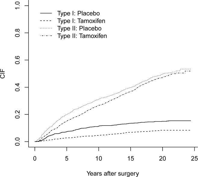
Estimated CIFs for tamoxifen vs placebo for the two types of events in the breast cancer data.

5.2 Analyses using subhazard models

For the data analysis we consider the three covariates of interest: treatment (x_ij1 is 1 for tamoxifen and 0 for placebo), age (x_ij2) and tumor size (x_ij3) as continuous covariates. Let v_i0 and v_i1 be random center effects and random treatment effects (i.e. random treatment-by-center interaction), respectively. Following Ha et al.¹⁰, we consider the three submodels of (1) for the time to Type 1 event, which include the proportional subhazards model without random effects (i.e. Fine-Gray model) and two subhazard frailty models. In other words, we consider the following three models, ${\mathrm{\lambda }}_{1ij}^s(t|v)={\mathrm{\lambda }}_{01}^s(t)\exp ({\eta }_{\mathit{ij}})$ with η_ij allowing two frailty structures (M2 and M3): Here (v_i0, v_i1) ~ BN means that $v_{i0}~N(0,{\sigma }_0^2)$, $v_{i1}~N(0,{\sigma }_1^2)$ and ρ = Corr(v_i0, v_i1).

• M1 (F-G): η_ij = β₁x_ij1 + β₂x_ij2 + β₃x_ij3;

• M2 (Center): η_ij = v_i0 + β₁x_ij1 + β₂x_ij2 + β₃x_ij3, with $v_{i0}~N(0,{\sigma }_0^2)$;

• M3 (Corr): η_ij = v_i0 + (β₁ + v_i1)x_ij1 + β₂x_ij2 + β₃x_ij3, with (v_i0, v_i1) ~ BN,

where ‘F-G’, ‘Center’ and ‘Corr’ indicate Fine-Gray model without frailties, subhazard frailty model with the random center effect v_i0 and subhazard correlated frailty model with ρ = Corr(v_i0, v_i1), respectively. Here M3 ( ${\sigma }_0^2>0$, ${\sigma }_1^2>0$, ρ ≠ 0) is our full model and the others are various simplifications of it by assuming null components, i.e. M1 (v_i0 = 0, v_i1 = 0; ${\sigma }_0^2=0$, ${\sigma }_1^2=0$) and M2 (v_i1 = 0; ${\sigma }_0^2>0$, ${\sigma }_1^2=0$). The estimation results are listed in Table 4.

Table 4.

Results for fitting the three subhazard models to Type 1 event of the breast cancer data

Model	Treatment ${\widehat{\beta }}_1$ (SE)	Age ${\widehat{\beta }}_2$ (SE)	Tumor size ${\widehat{\beta }}_3$ (SE)	${\widehat{\sigma }}_0^2$ (SE)	${\widehat{\sigma }}_1^2$ (SE)	${\widehat{\sigma }}_{01}[\widehat{\rho }]$ (SE)	$-2p_{\beta ,v}(h_w^{\ast })$
M1 (F-G)	−0.667 (0.119)	−0.026 (0.005)	0.082 (0.042)	–	–	–	4870.5
M2 (Center)	−0.672 (0.119)	−0.026 (0.005)	0.081 (0.042)	0.043 (0.051)	–	–	4869.4
M3 (Corr)	−0.658 (0.137)	−0.026 (0.005)	0.079 (0.043)	0.091 (0.026)	0.249 (0.073)	−0.108 [−0.721] (0.037)	4865.7

M1, proportional subhazard model (Fine-Gray model) without frailties;

M2, subhazard shared frailty model with random center effect only;

M3, subhazard correlated frailty model with ρ;

${\widehat{\sigma }}_0^2$ and ${\widehat{\sigma }}_1^2$, the variances of random center effect and random treatment-by-center interaction, respectively;

σ₀₁ and ρ, the corresponding covariance and correlation with ρ = σ₀₁/(σ₀σ₁);

SE, the estimated standard error for regression and frailty parameters;

$p_{\beta ,v}(h_w^{\ast })$, restricted h-likelihood in (9).

In all the three subhazard models the two fixed effects (β_j, j = 1, 2) are significant, except for β₃. In particular, the use of tamoxifen (tamoxifen = 1) significantly reduces the risk of local or regional recurrence (Type 1 event) as compared to patients who receive placebo (placebo= 0). We also observe that overall, there are no substantial changes in the fixed-effects estimates, although the effect of main treatment (β₁) becomes slightly weaker due to the increased standard error when the two random components and their correlation are included as in M3. In M2 and M3, the variance components ( ${\sigma }_0^2$ and ${\sigma }_1^2$) indicate the amount of variation between centers in baseline risk (i.e. center effect) and in the treatment effect, respectively. Here, the estimate and SE of ${\sigma }_1^2$ are relatively larger than those of ${\sigma }_0^2$, which is also confirmed in Figure 2. Furthermore, the correlated model M3 explains the degree of dependency between the two random components (i.e. the random center effect v₀ and the random treatment-by-center interaction v₁). The estimate of $\rho (\widehat{\rho }=-0.721)$ gives a negative value, indicating that the two predicted random components ( ${\widehat{v}}_0$ and ${\widehat{v}}_1$) have a negative correlation. In particular, the estimate of β₁ in M3 is negative; we see that a decreasing value of v_i1 corresponds to a larger treatment effect. Thus, the negative correlation leads to the conclusion that treatment confers more benefit in centers with a higher baseline risk. This is consistent with the findings by Rondeau et al.⁹ in the context of meta-analysis and by Ha et al.¹⁰ in that of multi-center trials.

Figure 2.

Random effects of 167 centers in the breast cancer data (event of interest is Type 1) and their 95% confidence intervals, under subhazard correlated frailty model (M3); (a) random center effects (v_i0); (b) random treatment-by-center interaction (i.e. random treatment effects) (v_i1); Centers are sorted in increasing order of number of patients.

5.3 Investigating and testing for heterogeneity

We demonstrate how to investigate heterogeneity related to treatment effect over centers using confidence intervals^17,18 for frailties of the individual centers. Note that the standard intervals using $p_{\tau }(h_w^{\ast })$ in (9) can be null due to zero estimation of the variance components, especially for small sample sizes or small variance components.^18,33,34 Thus we follow Ha et al.’s¹⁸ modification of (9) to deal with such shrinkage issue¹² for frailty. That is, for estimation of frailty parameters θ we use a further adjusted likelihood, defined by

$$p_{\text{adj}}=p_{\tau }(h_w^{\ast })+\log \det ({\sum }_i),$$ (14)

which leads to non-negative variance-component estimators. Following Ha et al.¹⁸ and (14), the individual (1 − α)-level h-likelihood confidence intervals for the unidimensional components v_k of random effects v are of the form

$${\widehat{v}}_k\pm z_{\alpha /2}·\text{SE}({\widehat{v}}_k-v_k),$$ (15)

where $\widehat{v}$ maximizes the profile h-likelihood $h_w^{\ast }$ in (7), z_α/2 is the normal quantile with probability α/2 in the right tail, and $\text{SE}({\widehat{v}}_k-v_k)$ are obtained from $H{(h_w^{\ast };\widehat{\beta },\widehat{v})}^{-1}$. In particular, Ha et al.¹⁸ have shown via numerical studies that in a general class of frailty models without competing risks, the adjusted h-likelihood interval (15) preserves well the nominal interval. Figure 2 shows the estimates and 95% confidence intervals^17,18 for the random effects in the 167 centers using the subhazard correlated model M3. Here, centers are ordered by the number of patients entered. Figures 2(a) and 2(b) give the confidence intervals for the random center effect (v_i0) and the random treatment-by-center interaction (v_i1), respectively. Overall, the lengths of the intervals are seen to decrease as the number of patients per center increases: see also Vaida and Xu⁸ and Ha et al.¹⁰.

Figure 2(a) indicates overall homogeneity in the baseline risk across 167 centers (i.e. no variation in random center effect). Figure 2(b) also shows there is no substantial variation in the effect of treatment across centers although three centers (148, 164 and 165) among 167 centers noticeably stand out. Note here that the centers (148, 165) and 164 provide the lowest and the highest treatment-by-center interactions, respectively, but that the corresponding three intervals include zero; this indicates there is little treatment-by-center interaction in this data set. Thus, in this multicenter trial there is little variation in the treatment effects across centers and the treatment is shown to be effective, These results suggest that the treatment effect may be generalized to a broader patient population as in the findings by Yamaguchi and Ohashi³⁵ and Ha et al.¹⁰

Now, we show this heterogeneity can also be tested via the restricted h-likelihood in (9). Recently, Katsahian and Boudreau²⁷ proposed how to test such heterogeneity (i.e. variation in random center effect) using the PPL method under the subhazard model (M2) with random center effect only. However, the heterogeneities from random treatment-by center interaction as well as random center effect should be simultaneously tested. For this purpose we again consider the three models in Section 5.2. Note that although we report the SEs of the σ²s in Table 4, one should not use them for testing $H_0:={\sigma }_0^2=0$.^{8, 10} Firstly, the null hypothesis $H_0:={\sigma }_0^2=0$ (i.e. no center effect) lies on the boundary of the parameter space. Consider the difference of deviance $-2p_{\beta ,v}(h_w^{\ast })$ between two models (M1 and M2). As shown in the simulation study of Section 4, under the null hypothesis this LR test statistic asymptotically follows a chi-square mixture $({\chi }_0^2+{\chi }_1^2)/2$.^10,32,36 From Table 4, we obtain the deviance difference between M1 and M2 to be 1.1 (p-value=0.147), indicating that the random center effect is not significant (i.e. ${\sigma }_0^2=0$). Furthermore, the difference in deviance between M2 and M3 is 3.7 (p-value=0.106) with an asymptotic $({\chi }_1^2+{\chi }_2^2)/2$ statistic³⁷, leading to ${\sigma }_1^2=0$. Accordingly, we find that there are no substantial variations for the baseline risk and treatment effect over centers, which confirms the homogeneity evident in Figure 2.

6 Discussion

We have shown that the proposed correlated frailty modelling approach based on the h-likelihood provides systematically more informative results for multi-center competing risk data. We have also demonstrated via a practical example how to investigate the heterogeneity related to treatment effect over centers and how to test such heterogeneity.

Our h-likelihood procedure can be also applied for fitting the cause-specific PH frailty models^7,38, by using the risk set in the classical Cox model. It would be an interesting comprehensive analysis to compare the inference results from both the sub-hazard and cause-specific frailty models for the Type 1 event in the breast cancer dataset presented in Section 5. We have shown via a simulation study that the LR tests based on the h-likelihood perform well under the subhazard shared frailty model (2) with one frailty parameter only. However, a simulation study under the subhazard frailty model (3) with a general correlation structure (4) might be challenging due to the number of parameters to be dealt with, and hence it would be an interesting future work. Another further work is to investigate the performance of the proposed method via a simulation study when the cluster size n_i is random or data-directed unbalanced case¹⁰ because in current simulation settings, n_i is always fixed and at least 10.

The subhazard frailty models (1) implicitly assume that the frailty effects for the event of interest are independent of those for the other types of events (i.e. competing events). Developing an extended frailty modelling approach to allow a correlation between both events would be an interesting topic for future work.

Appendix: Proof of estimating equations in (8)

The weighted partial h-likelihood $h_w^{\ast }$ in (7) can be expressed as

$$h_w^{\ast }=h_w{|}_{{\mathrm{\lambda }}_{01}^s={\widehat{\mathrm{\lambda }}}_{01}^w},$$ (16)

where h_w = ℓ_1w + Σ_iℓ_2i and ${\mathcal{l}}_{1w}={\sum }_k{d}_{(k)}\log {\mathrm{\lambda }}_{01k}^s+{\sum }_{\mathit{ij}}{\delta }_{\mathit{ij}}{\eta }_{\mathit{ij}}-{\sum }_{\mathit{ij}}{\mu }_{\mathit{ij}}$. Here ${\mu }_{\mathit{ij}}={\mathrm{\Lambda }}_{01}^s(y_{\mathit{ij}})w_{\mathit{ij}}\exp ({\eta }_{\mathit{ij}})$ with ${\mathrm{\Lambda }}_{01}^s(y_{\mathit{ij}})={\sum }_k{\mathrm{\lambda }}_{01k}^{s}I\{(i,j)\in R_{(k)}\}$, and

$${\widehat{\mathrm{\lambda }}}_{01k}^w(\beta ,v)=\frac{d_{(k)}}{{\sum }_{(i,j)\in R_{(k)}}{w}_{\mathit{ij}}\exp ({\eta }_{\mathit{ij}})},$$

are solutions of the estimating equations, $\partial h_w/\partial {\mathrm{\lambda }}_{01k}^s=0$, for k = 1, …, D. Thus, Ha et al.’s¹⁰ procedures for standard correlated frailty models without competing risks can be extended to the subhazard model (1) by using $h_w^{\ast }$ in (16). That is, given frailty parameters θ, the MHL estimators of τ = (β^T, v^T)^T are obtained by solving the joint estimating equations, $\partial h_w^{\ast }/\partial \tau =0$. Here, the calculations in Ha and Lee²⁶ and Ha et al.¹⁰ show that

$$\partial h_w^{\ast }/\partial \tau =\partial h_w/\partial \tau {|}_{{\mathrm{\lambda }}_{01}^s={\widehat{\mathrm{\lambda }}}_{01}^w}=\{E^T(\delta -\mu )-F\tau \}{|}_{{\mathrm{\lambda }}_{01}^s={\widehat{\mathrm{\lambda }}}_{01}^w}$$

since ∂h_w/∂τ = (∂η/∂τ)(∂h_w/∂η) with η = Xβ + Zv = Eτ. Here E = (X, Z), $F=\text{BD}(0,{\sum }_1^{-1},\dots ,{\sum }_q^{-1})$, and δ and μ are the n × 1 vectors of δ_ij’s, and μ_ij’s, respectively. Note that the vector μ can be written as a simple form by using a weighted risk indicator matrix M which contains the weight w_ij as well as the risk set R_(k). Let L be the n×1 vector of L_ij’s with $L_{\mathit{ij}}={\mathrm{\Lambda }}_{01}^s(y_{\mathit{ij}})w_{\mathit{ij}}$. Since ${\mathrm{\Lambda }}_{01}^s(y_{\mathit{ij}})={\displaystyle {\sum }_k{\mathrm{\lambda }}_{01k}^{s}I\{(i,j)\in R_{(k)}\}}$ and $w_{\mathit{ij}}=\widehat{G}(y_{(k)})/\widehat{G}(y_{\mathit{ij}}\wedge y_{(k)})$, we have L = MAJ, where M is the n × D weighted-risk indicator matrix whose (ij, k)th element is m_ij,k, $A=\text{diag}({\mathrm{\lambda }}_{01k}^s)$ is the D × D diagonal matrix and J is the D × 1 vector with one. This gives μ = W₀(MAJ) with W₀ = diag{exp(η_ij)}. Note here that m_ij,k are constructed by combining R_(k) and w_ij as in Ruan and Gray³⁰:

$$m_{ij,k}=I\{y_{\mathit{ij}}\ge y_{(k)}\text{or}(y_{\mathit{ij}}\le y_{(k)}\text{and}{\epsilon }_{\mathit{ij}}\ne 1)\}\{\widehat{G}(y_{(k)})/\widehat{G}(y_{\mathit{ij}}\wedge y_{(k)})\}=I\{y_{\mathit{ij}}\ge y_{(k)}\}+I\{y_{\mathit{ij}}\le y_{(k)}\text{and}{\epsilon }_{\mathit{ij}}\ne 1\}\{\widehat{G}(y_{(k)})/\widehat{G}(y_{\mathit{ij}})\}.$$ (17)

This is also equivalent to the weights by Katsahian et al.⁶ and Katsahian and Boudreau²⁷ because m_ij,k are equal to one as long as individuals have not failed by time y_(k) (i.e. y_ij ≥ y_(k)), and below 1 and decreasing over time if they failed from another type (Type 2) before y_(k) (i.e. y_ij ≤ y_(k) and ε_ij ≠ 1), and zero otherwise (e.g. they failed from Type 1 or have been right censored).

Furthermore, using the computation of Ha and Lee²⁶, we have

$$-{\partial }^2{h}_w^{\ast }/\partial {\tau }^2=E^T{W}^{\ast }E+F,$$ (18)

where W* = W₁ − W₂, W₁ = diag(μ), W₂ = (W₀M)C⁻¹(W₀M)^T, $C=\text{diag}\{d_{(k)}/{({\mathrm{\lambda }}_{01k}^s)}^2\}$ is the D × D diagonal matrix, and F = BD(0, U). Following Ha and Lee²⁶ and (18), we can show that given θ, the MHL estimators of τ = (β^T, v^T)^T are obtained from the following score equations:

$$(E^T{W}^{\ast }E+F)\widehat{\tau }=E^T{w}^{\ast },$$

leading to (8). Here w* = W*η + (δ − μ). Note here that the ${\mathrm{\lambda }}_{01k}^s$ terms in W* and w* are evaluated at their estimates ${\widehat{\mathrm{\lambda }}}_{01k}^w=d_{(k)}/M_k^T\psi$, where M_k is the kth component vector of M = (M₁, …, M_D) and ψ is the vector of exp(η_ij)’s. This completes the proof.

References

- 1.Pintilie M. Competing risks: A practical perspective. Wiley; 2006. [Google Scholar]
- 2.Prentice R, Kalbfleisch JD, Peterson AV, Flournoy N, Farewell VT, Breslow NE. The analysis of failure times in the presence of competing risks. Biometrics. 1978;34:541–554. [PubMed] [Google Scholar]
- 3.Fine JP, Gray RJ. A proportional hazards model for the subdistribution of a competing risk. Journal of the American Statstical Association. 1999;94:496–509. [Google Scholar]
- 4.Hougaard P. Analysis of Multivariate Survival Data. New York: Springer; 2000. [Google Scholar]
- 5.Duchateau L, Janssen P. The Frailty Models. New York: Springer; 2008. [Google Scholar]
- 6.Katsahian S, Resche-Rigon M, Chevret S, Porcher R. Analysing multicentre competing risk data with a mixed proportional hazards model for the subdistribution. Statistics in Medicine. 2006;25:4267–4278. doi: 10.1002/sim.2684. [DOI] [PubMed] [Google Scholar]
- 7.Christian NJ. PhD thesis. Department of Biostatistics, University of Pittsburgh; 2011. Hierarchical likelihood inference on clustered competing risk data. [DOI] [PMC free article] [PubMed] [Google Scholar]
- 8.Vaida F, Xu R. Proportional hazards model with random effects. Statistics in Medicine. 2000;19:3309–3324. doi: 10.1002/1097-0258(20001230)19:24<3309::aid-sim825>3.0.co;2-9. [DOI] [PubMed] [Google Scholar]
- 9.Rondeau V, Michiels S, Liquet B, Pignon JP. Investigating trial and treatment heterogeneity in an individual patient data meta-analysis of survival data by means of the penalized maximum likelihood approach. Statistics in Medicine. 2008;27:1894–1910. doi: 10.1002/sim.3161. [DOI] [PubMed] [Google Scholar]
- 10.Ha ID, Sylvester R, Legrand C, MacKenzie G. Frailty modelling for survival data from multi-centre clinical trials. Statistics in Medicine. 2011;30:2144–2159. doi: 10.1002/sim.4250. [DOI] [PMC free article] [PubMed] [Google Scholar]
- 11.Ripatti S, Palmgren J. Estimation of multivariate frailty models using penalized partial likelihood. Biometrics. 2000;56:1016–1022. doi: 10.1111/j.0006-341x.2000.01016.x. [DOI] [PubMed] [Google Scholar]
- 12.Therneau TM, Grambsch PM, Pankratz VS. Penalized survival models and frailty. Journal of Computational and Graphical Statistics. 2003;12:156–175. [Google Scholar]
- 13.Lee Y, Nelder JA. Hierarchical generalized linear models (with discussion) Journal of the Royal Statistical Society, Series B. 1996;58:619–678. [Google Scholar]
- 14.Lee Y, Nelder JA, Pawitan Y. Generalised Linear Models with Random Effects: Unified Analysis via h-Likelihood. Chapman and Hall; 2006. [Google Scholar]
- 15.Fisher B, Costantino J, Redmond C, et al. A randomized clinical trial evaluating tamoxifen in the treatment of patients with node-negative breast cancer who have estrogen receptor-positive tumors. New England Journal of Medicine. 1989;320:479–484. doi: 10.1056/NEJM198902233200802. [DOI] [PubMed] [Google Scholar]
- 16.Fisher B, Dignam J, Bryant J, et al. Five versus more than five years of tamoxifen therapy for breast cancer patients with negative lymph nodes and estrogen receptor- positive tumors. Journal of the National Cancer Institute. 1996;88:1529–1542. doi: 10.1093/jnci/88.21.1529. [DOI] [PubMed] [Google Scholar]
- 17.Lee Y, Nelder JA. Likelihood inference for models with unobservables: another view (with discussion) Statistical Science. 2009;24:255–293. [Google Scholar]
- 18.Ha ID, Vaida F, Lee Y. Interval estimation of random effects in proportional hazards models with frailties. Statistical Methods in Medical Research. 2013 doi: 10.1177/0962280212474059. Published online: 29/January/2013. [DOI] [PMC free article] [PubMed] [Google Scholar]
- 19.Ha ID, Lee Y, Song JK. Hierarchical likelihood approach for frailty models. Biometrika. 2001;88:233–243. [Google Scholar]
- 20.Ha ID, Lee Y, MacKenzie G. Model selection for multi-component frailty models. Statistics in Medicine. 2007;26:4790–4807. doi: 10.1002/sim.2879. [DOI] [PubMed] [Google Scholar]
- 21.Breslow NE. Discussion of Professor Cox’s paper. Journal of the Royal Statistical Society, Series B. 1972;34:216–217. [Google Scholar]
- 22.Fan J, Li R. Variable selection for Cox’s proportional hazards model and frailty model. The Annals of Statistics. 2002;30:74–99. [Google Scholar]
- 23.McGilchrist C. REML estimation for survival models with frailty. Biometrics. 1993;49:221–225. [PubMed] [Google Scholar]
- 24.Pintilie M. Analysing and interpreting competing risk data. Statistics in Medicine. 2007;26:1360–1367. doi: 10.1002/sim.2655. [DOI] [PubMed] [Google Scholar]
- 25.Kuk D, Varadhan R. Model selection in competing risks regression. Statistics in Medicine. 2013;32:3077–3088. doi: 10.1002/sim.5762. [DOI] [PubMed] [Google Scholar]
- 26.Ha ID, Lee Y. Estimating frailty models via Poisson hierarchical generalized linear models. Journal of Computational and Graphical Statistics. 2003;12:663–681. [Google Scholar]
- 27.Katsahian S, Boudreau C. Estimating and testing for center effects in competing risks. Statistics in Medicine. 2011;30:1608–1617. doi: 10.1002/sim.4132. [DOI] [PubMed] [Google Scholar]
- 28.Gray RJ. Flexible methods for analyzing survival data using splines, with applications to breast cancer prognosis. Journal of the American Statstical Association. 1992;87:942–951. [Google Scholar]
- 29.Verweij JM, Van Houwelingen HC. Penalized likelihood in Cox regression. Statistics in Medicine. 1994;13:2427–2436. doi: 10.1002/sim.4780132307. [DOI] [PubMed] [Google Scholar]
- 30.Ruan PK, Gray RJ. Analyses of cumulative incidence functions via nonparametric multiple imputation. Statistics in Medicine. 2008;27:5709–5724. doi: 10.1002/sim.3402. [DOI] [PubMed] [Google Scholar]
- 31.Ha ID, Noh M, Lee Y. Bias reduction of likelihood estimators in semiparametric frailty models. Scandinavian Journal of Statistics. 2010;37:307–320. [Google Scholar]
- 32.Self SG, Liang KY. Asymptotic properties of maximum likelihood estimators and likelihood ratio tests under nonstandard conditions. Journal of the American Statistical Association. 1987;82:605–610. [Google Scholar]
- 33.Morris CN. Mixed model prediction and small area estimation. Test. 2006;15:72–76. [Google Scholar]
- 34.Li H, Lahiri P. An adjusted maximum likelihood method for solving small area estimation problems. Journal of Multivariate Analysis. 2010;101:882–892. doi: 10.1016/j.jmva.2009.10.009. [DOI] [PMC free article] [PubMed] [Google Scholar]
- 35.Yamaguchi T, Ohashi Y. Investigating centre effects in a multi-centre clinical trial of superficial bladder cancer. Statistics in Medicine. 1999;18:1961–1971. doi: 10.1002/(sici)1097-0258(19990815)18:15<1961::aid-sim170>3.0.co;2-3. [DOI] [PubMed] [Google Scholar]
- 36.Ha ID, Lee Y. Multilevel mixed linear models for survival data. Lifetime Data Analysis. 2005;11:131–142. doi: 10.1007/s10985-004-5644-2. [DOI] [PubMed] [Google Scholar]
- 37.Verbeke G, Molenberghs G. The use of score test for inference on variance components. Biometrics. 2003;59:254–262. doi: 10.1111/1541-0420.00032. [DOI] [PubMed] [Google Scholar]
- 38.Gorfine M, Hsu L. Frailty-based competing risks model for multivariate survival data. Biometrics. 2011;67:415–426. doi: 10.1111/j.1541-0420.2010.01470.x. [DOI] [PMC free article] [PubMed] [Google Scholar]
Associated Data
This section collects any data citations, data availability statements, or supplementary materials included in this article.