

Abstract
Three basic electronic properties of molecules, electron density (ED), charge density (CD), and electrostatic potentials (ESP), are dependent on both atomic mobility and occupancy of components in the molecules. Small protein subunits may bind large macromolecular complexes with a reduced occupancy or an increased atomic mobility or both due to affinity‐based functional regulation, and so may substrates, products, cofactors, ions or solvent molecule to the active sites of enzymes. A quantitative theory is presented in this study that describes the dependence of atomic functions on atomic B‐factor in Fourier transforms of the corresponding maps. An application of this theory is described to an experimental ED map at 1.73‐Å resolution, and to an experimental CD map at 2.2‐Å resolution. All the three density functions are linearly proportional to occupancy when the structure factor F(000) term of Fourier transforms of experimental density maps is included. Upon application of this theory to both experimental CD and ESP maps recently reported for photosystem II‐light harvesting complex II supercomplex at 3.2‐Å resolution, the occupancy of two extrinsic protein subunits PsbQ and PsbP is determined to be 20.4 ± 0.2%, and the negative mean ESP value of vitreous ice displaced by the supercomplex on electron scattering path is estimated to be 3% of the mean ESP value of protein α‐helices.
Keywords: atomic mobility, electrostatic potential (ESP), charge density, electron density, electron microscopy (EM), photosystem II (PSII), supercomplex, light‐harvesting complex (LHC), PsbP, PsbQ
Introduction
The distribution of electron density (ED) around the stationary nuclei of neutral atoms in a molecule as well as the distribution of charge density (CD) is well understood, and both are distributed within van der Waals' (vdW) radii of atoms.1 With random Brownian motions of nuclei, both functions spread outwards through probability‐weighted averaging of all possible nuclear locations following Gaussian distributions, that is the convolution of the original functions with Gaussian functions.2 Fourier transforms of these functions are the product of atomic scattering factors and another Gaussian term characterized by atomic B‐factor. As B value increases, these functions are distributed with smaller peak values but wider ranges than the original functions are.
With sufficiently large B values, peaks for bonded atoms may be merged, resulting in unresolvable atomic shapes. A single logarithm–logarithm relationship exists in X‐ray crystallography between the lattice resolution of an experimental ED map and the Wilson B‐factor of the diffraction data.3 This study presents a quantitative theory to describe how the peak maximum for an atom in an ED map varies as a function of atomic B value at sub‐Å resolution, and then extends it to structures at much lower resolution. By using a statistical approach that relies on an accuracy of overall fitting of protein α‐helices for example into experimental maps, this method can bypass the requirement of sub‐Å resolution for accurate determination of each of all the atomic positions. This is particularly useful for de‐convolution of B‐factor and occupancy effects when the occupancy of some component (or some atom) in large macromolecular complexes varies. This theory can be extended to the atomic and molecular electrostatic potential (ESP) function if its absolute reference point is known, or can be used to determine the absolute reference point if it is unknown.
Results and Discussion
Quantitative theory on ED and ESP peak maxima
Atomic ED function is the Fourier transform of X‐ray atomic scattering factor convoluted with atomic B value or atomic mobility, which measures root‐mean‐squares of atomic motion <|r|2> through the relationship of B = 8π2<|r|2>. X‐ray scattering factor f(s) for any atom can be numerically expressed as a sum of four Gaussian terms plus a constant (or five Gaussian functions) as follows4, 5, 6:
| (1) |
where s is sinθ/λ, S = 2s = 2sinθ/λ=1/d, θ is half scattering angle, λ is wavelength in Å, d is resolution in Å, and ai are coefficients of Gaussian functions defined by the term bi with b 5 = 0. Fourier transform of Eq. (1) results in the peak maximum ρ(0) for the atom at r = 0 with atomic B‐factor B upon integration throughout the entire reciprocal space using its volume increment dτ,
| (2) |
When proper B value is included, the effect of Fourier series termination to the peak maximum can be minimized (see below).7, 8, 9, 10, 11 Each atom has its own characteristic ai and bj parameters.
When Eq. (2) is plotted for protein atoms [Fig. 1(A)], it is clear that peak maxima for neutral atoms of H, C, N, and O are sufficiently distinct even when atomic B‐factor increases to >50 Å2. The scattering factor of an atom at the zero‐scattering angle (i.e. the total number of electrons) for the given atom is the sum of all its five Gaussian coefficients ai. The H:C:N:O ratio of peak maxima approaches the asymptotic ratios of total electrons of each atom with increasing B‐factors, 1:6:7:8 when B ≫ bj. The difference in peak maxima between neutral O atom and its anion O‐ form is relatively small with their asymptotic ratio is 8:9. This theory can explain the experimental observations on a relationship between peak maxima and B‐factor values reported for atoms in an X‐ray crystal structure of lysozyme at 0.65‐Å resolution.12
Figure 1.

Peak maximum and B‐factor relationship. (A) Theoretical plot using Eq. 3. (B) Experimental plot for all the backbone O, N, and Cα atoms of E. coli catalase structure reported for 5BV2 (Ref. 16).
One reason for deviating from the theoretical ratio relationship among H:C:N:O atoms is due to crossover contributions from their bonding partners but not due to the spreading of individual atomic ED functions themselves away from the peaks as B value increases. For example, the contribution of C atom at H atom position in a C–H bond can be much larger than the contribution of H atom on itself, making peak for H atom invisible. The contribution of this kind can be estimated using similar integration but with r = d where d is the bond length between C and H atoms [i.e. spherical P(r) density function]. When atomic function is assumed to be spherically symmetric and the interference function is sinc function, that is sin[rS]/[rS], then the resulting ED function is as follows after integration.2
| (3) |
Equation (3) becomes Eq. (2) when r = 0. Both Eqs. (2) and (3) imply that density values are highly dependent on B value (and thereby on the effective resolution, see below).
Given the fact that electron scattering factor for an ion can be numerically fitted using five Gaussian terms for its neutral vdW component plus a Coulomb's charge component,13, 14 integration can be carried out for atomic ESP function ψ(r) as follows:
| (4) |
| (5) |
| (6) |
where c 0 is 0.023934 in atomic unit, a constant for the m 0 e 2/[8πh 2 ɛ 0] term, m 0 is the mass of stationary electron, e is the charge of electron, h is Planck constant, ɛ 0 is the dielectric constant in vacuum where this ion is located, and ΔZ is the atomic partial charge. It should be noted that the fitted ESP's Gaussian parameters for the neutral component of an ion are neither related to the fitted parameters for its ED structure factors, nor related to those of corresponding neutral atoms.13, 15 For neutral atoms, the atomic ESP structure factors can be fitted with four different Gaussian terms with no constant term.15
The above equations for both atomic ED and ESP functions suggest that peak values and shape functions are encoded differently as a function of resolution in their corresponding structure factors. By computationally adjusting B values during Fourier synthesis, one can alter the relative contribution of Coulomb's term to vdW's term. For Mg(II) cation and Cl‐ anion, Coulomb's terms increase relatively to their vdW's terms as B‐factor increases, that is Mg(II) becomes more positive and Cl‐ becomes more negative in ESP at low resolution than at high resolution. Thus, by examining peak maxima as a function of B factor (or resolution), one can gain insight into the Coulomb's component of a species in question, and thus its chemical identity.
Varying occupancy of an atom reduces its atomic functions linearly in all resolution ranges, but does not alter the shapes of its atomic functions. If two atoms of interest have different occupancies but the same B value, the ratio of peak maxima between the two atoms is independent of resolution. If two atoms of interest have different B values but the same occupancy, the ratio of peak maxima is dependent on resolution (and their B values).
Chemical identification of atoms in X‐ray crystallography at 1.73‐Å resolution
An analysis of peak maxima in the experimental ED for backbone atoms (O, N, and Cα) of E. coli catalase16, 17 reported for 5BV2 at 1.73‐Å resolution unambiguously shows that they indeed follow separate traces as a function of B‐factor values as expected from the theory (Fig. 1, Eq. (2)). In the most ordered part of the structure (particularly, the lowest B‐factor region) where atomic B‐factors are the same or similar, the order of the peak maxima is well defined: O > N > Cα atoms.
A reason for peak maxima for the pair of atoms of different types to disobey this order is due to large differences in their B‐factors. For example, for the peak maximum for N atom to be larger than that of O atom, an atomic B‐factor of N has to be smaller than that of O by >5 Å2; and for the peak maximum for C atom to be larger than that of N atom, an atomic B‐factor of C has to smaller than that of N by >10 Å2. These limits can be estimated after drawing horizontal lines in the experimental plot [Fig. 1(B)].
An implication of the above observation is that when the side chains of Asn, Gln, and His residues are accidentally flipped, the resulting incorrect assignment of atom type in the flipped side chains cannot be removed by adjusting their B‐factors during model refinement because it typically has restrained B‐factor differences of 1.5 Å2 between bonded atoms, and of 2.0 Å2 between bond‐angle related atoms. As a consequence, large positive residual peaks will appear at the positions of small atoms that were placed in the position that should be larger, and large negative peaks will appear at the positions of large atoms that should be smaller. Thus, these residual peaks will pinpoint to the modeling errors of this kind occurring at the swapped O and N atoms in the fragments Oδ1–Cγ–Nɛ2 of Asn side chain, and Oɛ1–Cδ–Nɛ2 of Gln side chain, and swapped N and C atoms in the fragment of Nδ1–Cɛ1–Nɛ2–Cδ2 of His side chain.
In fact, several significant residual peaks with the heights >5.5σ in residual difference Fourier maps between the data and model have indeed helped to identify a few remaining modeling errors associated with side chain flips near the end of model refinement of catalase reported for 5BV2.16, 17 The successful application of the peak maxima theory to that structure is due to very low noise levels in its residual maps when its crystallographic R‐factor and free R‐factor are very small (being 8.2% and 13.2%, respectively).16, 17 In this situation, model bias is insignificant. In the presence of significant model bias, the best estimation of B‐factor of the atom in question should be made using an average B from all of its surrounding atoms within 5 Å radius, and the best estimation of peak maximum of the atom is to use an atomic model with this atom deleted. Thus, this procedure can be used to unambiguously establish the chemical identity of the atom in question even before model refinement is fully completed.
The catalase structure just discussed is only one of a few examples in the PDB with very low R‐factors that do not suffer from severe model bias. There are other ways that one can obtain model‐independent experimental ED maps, one of which is de novo non‐crystallographic symmetry (NCS) averaging used in the E. coli YfbU particle structure determination (which contains 16‐fold NCS).18 When the same NCS averaging procedure was applied to another data set of the crystal for this particle at ∼ 1.95‐Å resolution using normalized or sharpened structure factors, the resulting NCS‐averaged maps can readily distinguish among O, N, and C atoms in many places in that structure as well as the added oxygen atoms during data collection, details of which will be described elsewhere.
Experimental charge density and partial charges of atoms at 2.2‐Å resolution
Previously, it was observed that the experimental ESP map along protein backbone is highly affected by atomic partial charges when the resolution of that map permits to see effects of individual peptide dipoles.19 For backbone atoms within each amino acid, variations of B‐factors may be ignored, and peak maxima in the experimental CD maps should mainly reflect variations of partial atomic charges. In the experimental ED maps, O > N > C, but in the observed CD maps, C ≫ O for carbonyl backbone atoms in both α‐helices and β‐strands when the experimental CD map is derived from the EMD‐4116 reported for β‐galactosidase at 2.2‐Å resolution20 (Fig. 2). This reflects the relative order of partial charges present in these atoms.
Figure 2.

Experimental CD map for β‐galactosidase derived from emd‐4116 at 2.2‐Å resolution (Ref. 20) for backbone atoms (N–Cα–C–O in blue, green, cyan, and red) of residues in α‐helices and β‐strands on relative scale. Along each of the N–Cα, Cα–C, and C–O bonds, experimental data are plotted in evenly divided 10 points.
Along the C=O direction in α‐helices, the maximal CD values appear between the two atoms but near C, but in β‐strands, the maximal CD values are on or near C atoms (Fig. 2). It remains unclear whether this distinction is related to the fact that backbone dipoles are aligned in α‐helices, but not in β‐strands. If this is so, environment‐related partial charges are significant. Residues I454 and I455 are next to one another, but the amplitude of peak variations in the experimental CD map between the C and O atoms differ greatly [Fig. 2(B)]. This difference should be mainly attributable to their different environments. Although the coordinate accuracy for individual atoms may not be sufficiently highly in this model, a striking similarity in distribution of the experimental CD maps along N–Cα, Cα–C, and C–O bonds in each residue highlights an accuracy of the overall fitting of secondary structures (Fig. 2).
Determination of subunit occupancy in 3.2‐Å resolution in cryo‐EM maps
The functional role of photosystem II (PSII) extrinsic proteins PsbO, PsbP, and PsbQ is to retain Ca2+ and Cl‐, two essential cofactors for photosynthetic oxygen evolution.21, 22, 23, 24 The binding of PsbQ to PSII within the spinach PSII–Light‐Harvesting Complex II (LHCII) supercomplex requires the co‐binding of PsbP. This supercomplex is dynamic, and subject to light‐dependent regulation. Both PsbQ and PsbP subunits can readily be dissociated from the supercomplex during a high‐salt wash procedure,25 making it possible to define their specific functions in the enzyme through in vitro reconstitution. In the sucrose gradient procedure described by Caffarri et al.,26 PsbQ is completely absent in band 7 (B7), but appears in B8, increases from B8 through B11, and then decreases after B11; and any excessive PsbP appears highly enriched in B1.
Wei et al., adopted the procedure of Caffarri et al. to purify the spinach PSII–LHCII supercomplex, and selected the B9 sample for cryo‐EM image reconstruction in which both PsbQ and PsbP subunits appear at sub‐stoichiometry of unknown molar ratio.26, 27 The actual stoichiometry of these subunits in the final EM map may also be affected by specific procedures of particle selection after EM images being made, which may enrich or deplete them in the supercomplex. Thus, it would be valuable to directly estimate their occupancy from the experimental data.
Within the PSII–LHCII supercomplex structure reported27 for 3JCU derived from EMD‐6617 at ∼3.2 Å resolution, subunits CP43 and PsbQ (subunit IDs of C and Q in the PDB of 3JCU) intimately interact with each other (Fig. 3, S1). At +2.0σ contour level of the experimental CD map3 derived from the ESP map,27 the volume inside the envelope of this contour level for PsbQ is estimated to be approximately the same to the volume inside that of the contour level of ∼+10.0σ for subunit CP43 according to visual inspection [Fig. 3(A)]. This volumetric relationship appears to be maintained as long as the ratio of contour level is kept about one‐to‐five for the two subunits in the CD map.
Figure 3.

Experimental CD map for subunits CP43 and PsbQ and comparison with the EM maps (Ref. 27). (A) CD maps contoured at +2.0σ (salmon) and +10.0σ (blue) with two helices from each subunit are zoomed out. (B–D) Comparison with the original unsharpened (left column), and sharpened (middle, B = −150Å2) ESP maps, and un‐sharped CD map (right), contoured at +1.3σ. Red arrows indicate the location of H120 of PsbQ in each map. Stereodiagrams are available in Supporting Information (Fig. S1).
At +1.3σ contour level, the entire PsbQ is visible in the CD map [Fig. 3(B–D)]. The CD map has a unique property: the volume in general does not extend beyond the vdW radii's of atoms in the molecule plus any atomic motions whereas the volume of the experimental ESP map does. Lowering contour from the +6.5σ to 1.3σ, the volume increases slowly and in similar amount for both CP43 and PsbQ. The spatial resolution for both subunits appears to remain relatively unchanged. For example, the curvature of helical path is clearly visible, but there is no carbonyl bump for both subunits visible at this resolution. This indicates that atomic motions for the two subunits within the supercomplex appear very similar, and that the differences observed here at different contour levels for the two subunits likely reflect their relative occupancy.
On the basis of the visual inspection method just described, the occupancy of PsbQ is estimated to be ∼20% in the supercomplex. This ratio remains similar when the CD maps are examined with computationally reduced resolution of 4.5 Å or 4.0 Å from 3.2 Å. The same occupancy of ∼20% is obtained for subunit PsbP (Fig. 4, S2) as well as for a region of the third extrinsic subunit PsbO comprising residues G236 to V276 (data not shown), which is partly buried underneath PsbP in the supercomplex.27 When PsbP is absent, this region of PsbO no longer appears to bind. The absence of PsbP does not affect the occupancy of the remaining part of PsbO in the supercomplex.
Figure 4.

Experimental CD map for subunits CP47 and PsbP contoured at +1.5σ (salmon) and +6.5σ (blue) (derived from Ref. 27). Views of the entire subunits are available in Supporting Information (Fig. S2).
To further quantify the occupancy, the experimental CD map is plotted in one dimension (1D) along the Cα–Cα line of consecutive backbone peptide units, and arranged in the tail‐to‐head manner for each of the two helices discussed above, one from CP43 and the other from PsbQ [Fig. 5(A,B)]. In this plot, the structure factor F CD(000) term for the CD map is set to be zero because the mean CD value for any large molecule should always be zero. Although the coordinate accuracy of each individual Cα atom may not be sufficiently high for the analysis of peak maxima of individual atoms, the accuracy of overall fitting of helices into the map should be statistically reasonable. According to the equations above, if a positive mean B‐factor difference between subunits PsbQ and CP43 does exist, the density ratio between them increases as the resolution of the Fourier transform reduces. However, the mean CD ratio over 26 residues is 20.2% at 3.2‐Å resolution, and it is 20.6% at computationally reduced 4.0‐Å resolution [Fig. 5(A,B)]. These two ratios are virtually identical, and the ratios of their mean values indeed represent the relative occupancy of subunit PsbQ in the supercomplex, but not likely a B‐factor difference.
Figure 5.
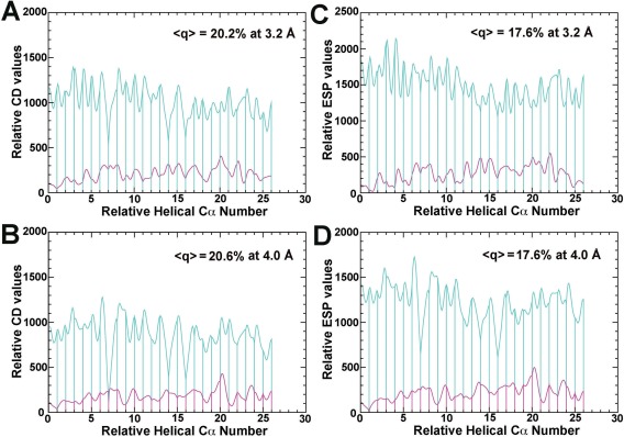
Experimental EM maps (Ref. 27) plotted along Cα–Cα line for helices (residues R154‐Y181, cyan; residues D99‐I124, magenta). Experimental CD maps (A, B) (no sharpening), and ESP maps/B = −150 Å2 (C, D) are calculated at 3.2‐Å resolution (A, C), and at computationally truncated resolution of 4.0 Å (B, D).
The method just described complements with existing crystallographic titration methods for binding‐affinity determination of cofactors in protein crystals.28, 29, 30 In previous methods, the asymptotic value represents the maximal density. In the current method, the maximal density is obtained using an internal reference point.
Mean ESP value of vitreous ice displaced by particles on electron scattering path
Given the known occupancy for subunit PsbQ determined from the experimental CD density above, one can estimate the mean ESP value of the displaced vitreous ice by particles along electron scattering path that was used to measure the EMD‐6617 map.27 It follows. If the structure factor F ESP(000) term is left out in the Fourier transform of the experimental ESP map [Fig. 5(C,D)], the entire ESP curve is shifted by a value of the F ESP(000)/volume ratio. After this shift, the ratio of the mean ESP value between subunits PsbQ and CP43 no longer equals the occupancy of PsbQ [Fig. 5(C,D)]. Through back‐extrapolation, the contribution of the F ESP(000) term is estimated to be ∼‐3.1% relative to the mean ESP value for the entire helix in subunit CP43. Thus, when the contribution of vitreous ice is omitted, the ESP maps have systematically been pushed upwards by 3.1% on average. The negative sign of mean ESP value for ice obtained here is consistent with the sign of the mean ESP value for liquid water previously measured experimentally (i.e., the mean Coulomb's ESP value of liquid water is ∼−900 mV),31 which should be applicable to vitreous ice.
Given the non‐zero ESP value of vitreous ice, varying length of ice displaced by particles affect the EM maps obtained for rectangle‐shaped particles (i.e. the PSII–LHCII supercomplex) far greater than those for the globular particles (i.e. the ribosomes) when the mean ESP values of surrounding ice are used as reference points. The PSII–LHCII supercomplex27 is a rectangle‐shaped transmembrane protein complex with the longest dimension of ∼260 Å approximately along x direction, the width of ∼140 Å along y direction, and shortest membrane dimension of ∼110 Å (or less for lipid bilayer only) along z direction. When projected along z axis, the effective length of electron scattering path of vitreous ice to be displaced by particles is ∼110 Å; and when projected along x axis, it is ∼260 Å. In these two orientations, the maximal length difference is ∼150 Å.
The value obtained for vitreous ice in this study represents an orientation average of all the particle dimensions weighted by orientation‐dependent sampling density (the bound lipid bilayers are part of the PSII–LHCII supercomplex assuming that they remain unchanged in different orientations). Given the large length difference just described, the image contrast for the same particle in these two orientations should differ greatly. Before these ESP images can be averaged after alignment, different zero‐reference points and different scaling factors should be applied.
It is well known that both the thickness of vitreous ice and the selection of specific particles within it are important for cryo‐EM analysis.32 The mean ESP value of water molecules in liquid and crystalline phases and in the vitreous ice form has been extensively studied, starting from the simple elegant, classic Coulson–Eisenberg treatment to more complex theoretical and experimental studies such as high‐energy electron holography.31, 32, 33, 34, 35, 36, 37 It remains an active research subject. It is also known that the mean ESP value of water molecules at the liquid–air interface is far greater than within liquid phase.37 If these observations are applicable to vitreous ice, which should be, an initial electrostatic interaction between this surface potential and an incident electron beam could generate a transient electric force field. This field can then be converted to a mechanic force to cause movements of ice before it finds a new equilibrium position. The displacement motions of ice have indeed been observed, and can be delineated using a dose‐fractionated, ice displacement‐corrected, image reconstruction method.38
The relationship between atomic B‐factor and resolution
In crystallography, lattice resolution is a property of entire data set, related to the Wilson B‐factor of the data set. It is also related to the mean B value of the underlying macromolecular structure in crystal. Some atoms in the structure will have larger B values than the mean, and other will have smaller. Fourier transformation used in model refinement and map calculation is often carried out at one‐third of the lattice spacing, instead of the minimal Nyquist frequency of one half. Although how this rule‐of‐thumb principle in Fourier transformation affects the B‐factor distribution of atoms in models being refined remains unknown, it can partly minimize computational errors for atoms with very small B‐factors. The term atomic resolution is traditionally defined in X‐ray crystallography, typically at sub‐Å lattice spacing, such that the chemical identity of an atom in question can be established unambiguously from the ED peak maximum, ρ(0), and the shape function, ρ(r), at any non‐zero r value relative to its nucleus.1
The effect of possible resolution underestimation in protein crystallography39 on the ED peak maximum for an atom of given B‐factor can be numerically estimated using error‐free simulation (see Methods), that is the percentage contribution of the Fourier terms to the peak maximum beyond the maximal resolution S max that are omitted in calculation. The results obtained show that for any given percentage, the slope of ln[S max] versus ln[B] is approximately ½ for both this error‐free simulation and the experimental data3, 39 because the product B[S max]2 term is dimensionless (Fig. 6). According to this simulation, on average, peak maxima obtained in macromolecular crystallography only represent ∼80% of their theoretical values. The effect of resolution underestimation on atoms with small atomic B factors is much higher than those with large B factors.
Figure 6.

Experimental (black solid line) and simulated (dashed lines) relationship between the maximal resolution S max = 1/d max, and Wilson B‐factor of a data set. (A) The S max versus B plot. (B) The ln[S max] versus ln[B] plot.
The results obtained in this study should not be affected by possible errors in numerically fitted Eqs. (1) and (4). These equations are broken down when sinθ/λ > 2.0, and alternative formulations have been proposed.5 However, very high‐scattering angle data are not practically relevant when they are not experimentally measurable because of Debye–Waller factors.40
The resolution of cryo‐EM maps being reported differs somewhat from one used in crystallography. It tends to be claimed higher than in crystallography so that no information will not be lost when the minimal Nyquist frequency of ½ is used for Fourier sampling. It should be a concern when the molecular functions of the same atomic model with the same mean B‐factor are claimed to have very different resolutions. In fact, the term resolution has been abused commonly in structural biology,41, 42 where terms like super‐resolution, atomic resolution, or near‐atomic resolution often have nothing to do with reality. Atomic‐resolution electron microscopy does exist and emerges in material sciences, that is atomic ESP shape function can indeed be experimentally visualized;43 and that physically differs from what is being currently claimed in the cryo‐EM community for macromolecules.
Methods
Experimental CD maps were calculated from ESP maps as described previously.3 Structure factors for corresponding Fourier transforms were obtained using the programs CCP4 and Phenix,44, 45 which were used for recalculation of maps in any non‐grid point through direct Fourier summation. 1D plots along Cα–Cα line and N–Cα, Cα–C, and C–O bonds are calculated using 10 evenly divided points between start and end points. The experimental map reported for EMD‐4116 was aligned onto EMD‐2984 using Chimera so that the model 5A1A derived from EMD‐2984 could be used to analyze the CD features derived from the realigned EMD‐4166 ESP maps.20, 46, 47
A stationary phenylalanine amino acid is placed in P1 unit cell with a = b=c = 20 Å and α = β = γ = 90°, and its error‐free X‐ray structure factors are calculated to a resolution of 0.2 Å and sorted in the descending order of reciprocal resolution, S = 1/d. The magnitude of the Fourier transform at its Cβ atom position is calculated using terms with the descending order of reciprocal resolution and is compared with the total Fourier transform of the crystal at this position as a function of atomic B‐factor. This calculation can be represented in formulation as follows.
| (7) |
| (8) |
In the above two equations, ρ(0) represents the peak value of the total Fourier transform at the Cβ coordinate, ρS max(0,B) is the peak value using the terms within the resolution limit S max = 1/d max, O(B,S max) is the Fourier transform of the omitted high‐resolution terms beyond the resolution limit, δ(B,S max) represents the percentage contribution of the omitted terms, and f(S) is the X‐ray structure factors (or X‐ray scattering factor). When the percentage of the omitted Fourier transform δ(B,S max) reaches 1%, 3%, 5%, 10%, 15%, and 20% of the total Fourier transform, the reciprocal resolution cut‐off S max is obtained for a given B value. The results are then plotted in the form of S max versus B and in the natural logarithm form of ln[S max] versus ln[B], and are compared with the experimental data adopted from recent studies (Fig. 6).3, 39 The results obtained here are independent of specific molecule used in this study, or specific atomic coordinates, or the upper limit of 0.2‐Å resolution used in the study. All of them only affect the accuracy of the plots in a small region of very small B‐factor with B < 2.5 Å2.
Supporting information
Supporting Information
Acknowledgments
The author thanks Professor Xinzheng Zhang for providing the information of the B‐factor value (‐150 Å2) used to sharpen their ESP map (EMD‐6617).
Conflict of interest statement: The author declares that he has no conflict of interest.
References
- 1. Bader RFW (1990) Atoms in molecules: a quantum theory. Oxford, New York: Clarendon Press. [Google Scholar]
- 2. Moore P ( 2012) Visualizing the invisible: imaging techniques for the structural biologist. Oxford, New York: Oxford University Press. [Google Scholar]
- 3. Wang J (2017) Experimental charge density from electron microscopic maps. Protein Sci 26:1619–1626. [DOI] [PMC free article] [PubMed] [Google Scholar]
- 4. Cromer DT, Mann JB (1968) X‐ray scattering factors computed from numerical Hartree‐Fock wave functions. Los Alamos Scientific Laboratory Report LA‐3816.
- 5. Fox AG, O'Keefe MA, Tabbernor MA (1989) Relativistic Hartree‐Fock X‐ray and electron atomic scattering factors at high angles. Acta Cryst A45:786–793. [Google Scholar]
- 6. Waasmaier D, Kirfel A (1989) New analytic scattering‐factor functions for free atoms and ions. Acta Cryst A51:416–431. [Google Scholar]
- 7. Sakurai T (1967) Peak heights of electron density and Patterson function in crystal. Acta Cryst 23:862–865. [Google Scholar]
- 8. Scheringer C (1977) Simple method of estimating effects of series termination and thermal smearing on peak heights. Acta Cryst A 33:588–592. [Google Scholar]
- 9. Scheringer C (1977) Temperature factors for internuclear density units. 2. Considerations with respect to experimental accuracy. Acta Cryst A 33:430–433. [Google Scholar]
- 10. Scheringer C (1977) Temperature factors for internuclear density units. 1. Theory in harmonic approximation. Acta Cryst A 33:426–429. [Google Scholar]
- 11. Scheringer C (1977) Interpretation of anisotropic temperature factors. 3. Anharmonic motions. Acta Cryst A 33:879–884. [Google Scholar]
- 12. Wang J, Dauter M, Alkire R, Joachimiak A, Dauter Z (2007) Triclinic lysozyme at 0.65 A resolution. Acta Cryst D 63:1254–1268. [DOI] [PubMed] [Google Scholar]
- 13. Peng LM (1998) Electron scattering factors of ions and their parameterization. Acta Cryst A 54:481–485. [Google Scholar]
- 14. Peng LM, Dudarev SL, Whelan MJ (1998) Electron scattering factors of ions and dynamical RHEED from surfaces of ionic crystals. Phys Rev B 57:7259–7265. [Google Scholar]
- 15. Peng LM (1999) Electron atomic scattering factors and scattering potentials of crystals. Micron 30:625–648. [Google Scholar]
- 16. Wang J, Lomkalin IV (2015) Crystal structure of E. coli HPII catalase variant. PDB entry released on 2015‐06‐24.
- 17. Wang J (2017) Systematic analysis of residual density suggests that a major limitation in well‐refined X‐ray structures of proteins is the omission of ordered solvent. Protein Sci 26:1012–1023. [DOI] [PMC free article] [PubMed] [Google Scholar]
- 18. Wang J, Wing RA (2014) Diamonds in the rough: a strong case for the inclusion of weak‐intensity X‐ray diffraction data. Acta Cryst D 70:1491–1497. [DOI] [PMC free article] [PubMed] [Google Scholar]
- 19. Wang J, Videla PE, Batista VS (2017) Effects of aligned alpha‐helix peptide dipoles on experimental electrostatic potentials. Protein Sci 26:1692–1697. [DOI] [PMC free article] [PubMed] [Google Scholar]
- 20. Bartesaghi A, Merk A, Banerjee S, Matthies D, Wu X, Milne JL, Subramaniam S (2015) 2 A resolution cryo‐EM structure of beta‐galactosidase in complex with a cell‐permeant inhibitor. Science 348:1147–1151. [DOI] [PMC free article] [PubMed] [Google Scholar]
- 21. Roose JL, Frankel LK, Mummadisetti MP, Bricker TM (2016) The extrinsic proteins of photosystem II: update. Planta 243:889–908. [DOI] [PubMed] [Google Scholar]
- 22. Ifuku K (2014) The PsbP and PsbQ family proteins in the photosynthetic machinery of chloroplasts. Plant Physiol Biochem 81:108–114. [DOI] [PubMed] [Google Scholar]
- 23. Bricker TM, Frankel LK (2011) Auxiliary functions of the PsbO, PsbP and PsbQ proteins of higher plant Photosystem II: a critical analysis. J Photochem Photobiol B 104:165–178. [DOI] [PubMed] [Google Scholar]
- 24. Ifuku K, Ido K, Sato F (2011) Molecular functions of PsbP and PsbQ proteins in the photosystem II supercomplex. J Photochem Photobiol B 104:158–164. [DOI] [PubMed] [Google Scholar]
- 25. Seidler A (1994) Expression of the 23 kDa protein from the oxygen‐evolving complex of higher plants in Escherichia coli. Biochim Biophys Acta 1187:73–79. [DOI] [PubMed] [Google Scholar]
- 26. Caffarri S, Kouril R, Kereiche S, Boekema EJ, Croce R (2009) Functional architecture of higher plant photosystem II supercomplexes. EMBO J 28:3052–3063. [DOI] [PMC free article] [PubMed] [Google Scholar]
- 27. Wei X, Su X, Cao P, Liu X, Chang W, Li M, Zhang X, Liu Z (2016) Structure of spinach photosystem II–LHCII supercomplex at 3.2 A resolution. Nature 534:69–74. [DOI] [PubMed] [Google Scholar]
- 28. Wang J, Yu P, Lin TC, Konigsberg WH, Steitz TA (1996) Crystal structures of an NH2‐terminal fragment of T4 DNA polymerase and its complexes with single‐stranded DNA and with divalent metal ions. Biochemistry 35:8110–8119. [DOI] [PubMed] [Google Scholar]
- 29. Gao Y, Yang W (2016) Capture of a third Mg(2)(+) is essential for catalyzing DNA synthesis. Science 352:1334–1337. [DOI] [PMC free article] [PubMed] [Google Scholar]
- 30. Nakamura T, Zhao Y, Yamagata Y, Hua YJ, Yang W (2012) Watching DNA polymerase eta make a phosphodiester bond. Nature 487:196–201. [DOI] [PMC free article] [PubMed] [Google Scholar]
- 31. Gabdoulline RR, Zheng C, Vanderkooi G (1997) The mean electrostatic potential difference between liquid water and vacuum by MD simulation. J Mol Liq 71:1–10. [Google Scholar]
- 32. Feja B, Aebi U (1999) Determination of the inelastic mean free path of electrons in vitrified ice layers for on‐line thickness measurements by zero‐loss imaging. J Microsc‐Oxford 193:15–19. [DOI] [PubMed] [Google Scholar]
- 33. Coulson CA, Eisenberg D (1966) Interactions of H2O molecules in ice. I. Dipole moment of an H2O molecule in ice. Proc R Soc Lon Ser A 291:445–453. [Google Scholar]
- 34. Coulson CA, Eisenberg D (1966) Interactions of H2O molecules in ice. 2. Interaction energies of H2O molecules in ice. Proc R Soc Lon Ser A 291:454–459. [Google Scholar]
- 35. Takahashi T (1969) Electric potential of liquid water on an ice surface. J Atmos Sci 26:1253–1258. [Google Scholar]
- 36. Takahashi T (1969) Electric potential of a rubbed ice surface. J Atmos Sci 26:1259–1265. [Google Scholar]
- 37. Kathmann SM, Kuo IFW, Mundy CJ, Schenter GK (2011) Understanding the surface potential of water. J Phys Chem B 115:4369–4377. [DOI] [PubMed] [Google Scholar]
- 38. Li X, Mooney P, Zheng S, Booth CR, Braunfeld MB, Gubbens S, Agard DA, Cheng Y (2013) Electron counting and beam‐induced motion correction enable near‐atomic‐resolution single‐particle cryo‐EM. Nat Methods 10:584–590. [DOI] [PMC free article] [PubMed] [Google Scholar]
- 39. Wang J (2015) Estimation of the quality of refined protein crystal structures. Protein Sci 24:661–669. [DOI] [PMC free article] [PubMed] [Google Scholar]
- 40. Peng LM, Ren G, Dudarev SL, Whelan MJ (1996) Debye‐Waller factors and absorptive scattering factors of elemental crystals. Acta Cryst A 52:456–470. [Google Scholar]
- 41. Wlodawer A, Dauter Z (2017) 'Atomic resolution': a badly abused term in structural biology. Acta Cryst D 73:379–380. [DOI] [PMC free article] [PubMed] [Google Scholar]
- 42. Chiu W, Holton J, Langan P, Sauter NK, Schlichting I, Terwilliger T, Martin JL, Read RJ, Wakatsuki S (2017) Responses to 'Atomic resolution': a badly abused term in structural biology. Acta Cryst D 73:381–383. [DOI] [PubMed] [Google Scholar]
- 43. Urban KW (2009) Is science prepared for atomic‐resolution electron microscopy?. Nat Mater 8:260–262. [DOI] [PubMed] [Google Scholar]
- 44. Winn MD, Ballard CC, Cowtan KD, Dodson EJ, Emsley P, Evans PR, Keegan RM, Krissinel EB, Leslie AGW, McCoy A, McNicholas SJ, Murshudov GN, Pannu NS, Potterton EA, Powell HR, Read RJ, Vagin A, Wilson KS (2011) Overview of the CCP4 suite and current developments. Acta Cryst D 67:235–242. [DOI] [PMC free article] [PubMed] [Google Scholar]
- 45. Adams PD, Afonine PV, Bunkoczi G, Chen VB, Davis IW, Echols N, Headd JJ, Hung LW, Kapral GJ, Grosse‐Kunstleve RW, McCoy AJ, Moriarty NW, Oeffner R, Read RJ, Richardson DC, Richardson JS, Terwilliger TC, Zwart PH (2010) PHENIX: a comprehensive Python‐based system for macromolecular structure solution. Acta Cryst D 66:213–221. [DOI] [PMC free article] [PubMed] [Google Scholar]
- 46. Yang Z, Lasker K, Schneidman‐Duhovny D, Webb B, Huang CC, Pettersen EF, Goddard TD, Meng EC, Sali A, Ferrin TE (2012) UCSF Chimera, MODELLER, and IMP: an integrated modeling system. J Struct Biol 179:269–278. [DOI] [PMC free article] [PubMed] [Google Scholar]
- 47. Kimanius D, Forsberg BO, Scheres SH, Lindahl E (2016) Accelerated cryo‐EM structure determination with parallelisation using GPUs in RELION‐2. Elife 5:e18722. [DOI] [PMC free article] [PubMed] [Google Scholar]
Associated Data
This section collects any data citations, data availability statements, or supplementary materials included in this article.
Supplementary Materials
Supporting Information