Controlling mRNA Translation

Abstract

The ribosomal density along different parts of the coding regions of the mRNA molecule affect various fundamental intracellular phenomena including: protein production rates, global ribosome allocation and organismal fitness, ribosomal drop off, co-translational protein folding, mRNA degradation, and more. Thus, regulating translation in order to obtain a desired ribosomal profile along the mRNA molecule is an important biological problem.

We study this problem using a dynamical model for mRNA translation, called the ribosome flow model (RFM). In the RFM, the mRNA molecule is modeled as chain of n sites. The n state-variables describe the ribosomal density profile along the mRNA molecule, whereas the transition rates from each site to the next are controlled by n + 1 positive constants. To study the problem of controlling the density profile, we consider some or all of the transition rates as time-varying controls.

We consider the following problem: given an initial and a desired ribosomal density profile in the RFM, determine the time-varying values of the transition rates that steer the system to this density profile, if they exist. More specifically, we consider two control problems. In the first, all transition rates can be regulated and the goal is to steer the ribosomal density profile and the protein production rate from a given initial value to a desired value. In the second, a single transition rate is controlled and the goal is to steer the production rate to a desired value. In the first case, we show that the system is controllable, i.e. the control is powerful enough to steer the system to any desired value, and we provide simple closed-form expressions for constant control functions (or transition rates) that asymptotically steer the system to the desired value. In the second case, we show that we can steer the production rate to any desired value in a feasible region determined by the other constant transition rates. We discuss some of the biological implications of these results.

I. Introduction

The process in which the genetic information coded in the DNA is transformed into functional proteins is called gene expression. It consists of two major steps: transcription of the DNA code into messenger RNA (mRNA) by RNA polymerase, and translation of the mRNA into proteins. During the translation step, macro-molecules called ribosomes unidirectionally traverse the mRNA, decoding it codon by codon into a corresponding chain of amino-acids that is folded co-translationally and post-translationally to become a functional protein. The rate in which proteins are produced during the translation step is called the protein translation rate or protein production rate.

Translation takes place in all organisms and tissues under almost all conditions. Thus, developing a better understanding of how translation is regulated has important implications to many scientific disciplines, including medicine, evolutionary biology, and synthetic biology. Developing and analyzing computational models of translation may provide important insights on this biological process. Such models can also aid in integrating and analyzing the rapidly increasing experimental findings related to translation (see, e.g., [8], [51], [41], [6], [45], [10], [36]).

Controlling the expression of heterologous genes in a host organism in order to synthesize new proteins, or to improve certain aspects of the host fitness, is an essential challenge in biotechnology and synthetic biology [40], [29], [3], [52], [2]. Computational models of translation are particularly important in this context, as they allow simulating and analyzing the effect of various manipulations of the gene expression machinery and/or the genetic material, and can thus save considerable time and effort by guiding biologists towards promising experimental directions.

The ribosome flow along the mRNA is regulated by various translation factors (e.g., initiation and elongation factors, tRNA and Aminoacyl tRNA synthetase concentrations, and amino-acid concentrations) in order to achieve both a suitable ribosomal density profile along the mRNA, and a desired protein production rate. Indeed, it is known that the ribosomal density profile and the induced ribosome speed profile along the mRNA molecule can affect various fundamental intracellular phenomena. For example, it is known that the folding of translated proteins may take place co-translationally, and inaccurate translation speed can contribute to protein miss-folding [12], [22], [55]. It is also known that the profile of ribosome density may affect the degradation of mRNA, ribosomal collisions, abortion and allocation, transcription, and more [12], [22], [23], [13], [55], [52], [35].

Thus, a natural question is whether it is possible, by controlling the transition rates along the mRNA, to steer the ribosome density along the mRNA molecule from any initial profile to any desired profile in finite time. In the language of control theory, the question is whether the system is controllable (see, e g. [48]). Controllability of networked systems is recently attracting considerable interest (see e.g. [24]). An important problem in this context is to determine a minimal set of “driver nodes” within the network such that controlling these nodes makes the entire network controllable (see e.g. [30]).

Controllability of mRNA translation is also important in synthetic biology, e.g. in order to design cis or trans intra-cellular elements that yield a desired ribosome density profile (or to determine if such a design is possible). Another related question arises in evolutionary systems biology, namely, determine if a certain translation-related phenotype can be obtained by evolution.

Our study is also related to cancer evolution. Indeed, it is well-known that cancerous cells undergo evolution that modulates their translation regime. It has been suggested that various mutations that accumulate during tumorigenesis may affect both translation initiation [16], [25] and elongation [53], [50] of genes related to cell proliferation, metabolism, and invasion. Specifically, the results reported in the recent study [16] support the conjecture that cancerous mutations can significantly change the ribosome density profile on the mRNAs of dozen of genes.

The standard mathematical model for ribosome flow is the totally asymmetric simple exclusion process (TASEP) [46], [56]. In this model, particles hop unidirectionally along an ordered lattice of L sites. Every site can be either free or occupied by a particle, and a particle can only hop to a free site. This simple exclusion principle models particles that have “volume” and thus cannot overtake one other. The hops are stochastic and the rate of hoping from site i to site i + 1 is denoted by γ_i. A particle can hop to [from] the first [last] site of the lattice at a rate α [β]. The flow through the lattice converges to a steady-state value that depends on L and the parameters α, γ₁,…, γ_L−1, β. In the context of translation, the lattice models the mRNA molecule, the particles are ribosomes, and simple exclusion means that a ribosome cannot overtake a ribosome in front of it. TASEP has become a fundamental model in non-equilibrium statistical mechanics, and has been applied to model numerous natural and artificial processes [44].

The ribosome flow model (RFM) [39] is a deterministic model for translation that can be derived via a dynamic mean-field approximation of TASEP [44, section 4.9.7] [4, p. R345]. In the RFM, mRNA molecules are coarse-grained into n consecutive sites of codons (or groups of codons). The state variable x_i(t): ℝ₊ → [0, 1], i = 1, …, n, describes the normalized ribosomal occupancy level (or density) of site i at time t, where x_i(t) = 1 [x_i(t) = 0] indicates that site i is completely full [empty] at time t. Thus, the vector [x₁(t) … x_n (t)]′ describes the complete ribosomal density profile along the mRNA molecule at time t. A variable denoted R(t) describes the protein production rate at time t. A nonnegative parameter λ_i, i = 0, …, n, controls the transition rate from site i to site i + 1, where λ₀ [λ_n] is the initiation [exit] rate.

In order to better understand how translation is regulated, we consider the RFM with some or all of the constant transition rates replaced by time-varying control functions that take non-negative values for all time t. The idea here that we can control these functions as desired.

We consider two control problems. In the first, all the n + 1 λ_is are replaced by control functions and the problem is to control these functions such that the ribosomal density profile and the production rate are steered from a given initial value to a desired value. We use the term “augmented profile” to indicate the combination of the ribosomal density profile and the production rate. In the second control problem, a single λ_i is replaced by a control u(t) and the problem is to control u(t) such that the production rate is steered to a desired value. Note that in the first problem the n + 1-dimensional vector describing the augmented profile is controlled using n + 1 control functions, and in the second problem a single variable is controlled using a scalar control.

We show that in both cases the resulting control system is controllable, i.e. the control is always “powerful” enough to steer the system from any initial state to any desired state in finite time. We also show that there always exists a control that steers the system as desired, and is the time concatenation of two controls:

$$u(t)=\{\begin{array}{ll}v,\hfill & t\in [0,T-\epsilon ),\hfill \\ w(t),\hfill & t\in [T-\epsilon ,T],\hfill \end{array}$$ (1)

with ε > 0 and very small. The constant control v is given in a simple and explicit expression that depends only on the desired final state. It guarantees that this state becomes the unique attracting steady-state ribosomal density and production rate of the RFM dynamics. For example, in the problem of controlling the density profile and the production rate to desired final values x^f and R^f respectively (“f” for final), the solution of the controlled RFM for any initial condition x(0) and R(0) satisfies

$$\underset{t\to \text{∞}}{\text{lim}}x(t)=x^f,$$

$$\underset{t\to \text{∞}}{\text{lim}}R(t)=R^f.$$ (2)

This means that for all practical reasons, one may simply apply the constant control u(t) ≡ v for all t > 0. Note that means that the exact values of x(0) and R(0), i.e. the initial values of the density profile and production rate, are actually not needed. This is important, as accurately measuring x(0) and R(0) in practice may be difficult. The control w(t) in is needed only to guarantee that x(T) = x^f and R(T) = R^f for some finite time T. The existence of such a w(t) follows from standard accessibility arguments, but w(t) is not given explicitly.

Different aspects of translation regulation, usually under natural conditions, have been studied before (see, for example, [17]). There are also a few studies on experimental and computational heuristics for mRNA translation engineering and optimization (see, for example, [43], [49]), and studies related to the way translation regulation is encoded in the transcript (e.g. [57], [32]). However, to the best of our knowledge, this is the first study on controlability of translation in a realistic model for translation. Also, previous studies on translation optimization only considered protein levels or production rate (e.g. [43]), but not the problem of controlling the entire profile of mRNA decoding rates as is done here.

The remainder of this paper is organized as follows. The following section provides a brief overview of the RFM and its generalizations into a control system. In order to make this paper accessible to a larger audience, Appendix A provides a very brief review of controllability, while demonstrating some of the concepts using the RFM. Section III presents our main results on the controlled RFM. We also discuss the biological ramifications of our results. To streamline the presentation, all the proofs are placed in Appendix B.

II. Ribosome Flow Model

In this section, we quickly review the RFM and describe its generalizations into a control system. The dynamics of the RFM with n sites is given by n non-linear first-order ordinary differential equations:

$${\dot{x}}_1={\mathrm{\lambda }}_0(1-x_1)-{\mathrm{\lambda }}_1{x}_1(1-x_2),$$

$${\dot{x}}_2={\mathrm{\lambda }}_1{x}_1(1-x_2)-{\mathrm{\lambda }}_2{x}_2(1-x_3),$$

$${\dot{x}}_3={\mathrm{\lambda }}_2{x}_2(1-x_3)-{\mathrm{\lambda }}_3{x}_3(1-x_4),$$

$$⋮$$

$${\dot{x}}_{n-1}={\mathrm{\lambda }}_{n-2}{x}_{n-2}(1-x_{n-1})-{\mathrm{\lambda }}_{n-1}{x}_{n-1}(1-x_n),$$

$${\dot{x}}_n={\mathrm{\lambda }}_{n-1}{x}_{n-1}(1-x_n)-{\mathrm{\lambda }}_n{x}_n.$$ (3)

If we define x₀(t): = 1 and x_n+1(t):= 0 then (3) can be written more succinctly as

$$\begin{array}{cc}{\dot{x}}_i={\mathrm{\lambda }}_{i-1}{x}_{i-1}(1-x_i)-{\mathrm{\lambda }}_i{x}_i(1-x_{i+1}),& i=1,\dots ,n\end{array}.$$ (4)

Recall that the state variable x_i(t): ℝ₊ → [0, 1] describes the normalized ribosomal occupancy level (or density) of site i at time t, where x_i(t) = 1 [x_i(t) = 0] indicates that site i is completely full [empty] at time t. Eq. (4) can be explained as follows. The flow of ribosomes from site i to site i + 1 is λ_ix_i(t)(1 − x_i+1(t)). This flow is proportional to x_i(t), i.e. it increases with the occupancy level at site i, and to (1 − x_i+1(t)), i.e. it decreases as site i + 1 becomes fuller. This corresponds to a “soft” version of the simple exclusion principle in TASEP. Note that the maximal possible flow from site i to site i + 1 is the transition rate λ_i. Eq. (4) thus states that the time derivative of state-variable x_i is the flow entering site i from site i − 1, minus the flow exiting site i to site i + 1.

The ribosome exit rate from site n at time t is equal to the protein production rate at time t, and is denoted by R(t):= λ_nx_n(t) (see Fig. 1). Note that x_i is dimensionless, and every rate λ_i has units of 1/time.

Fig. 1.

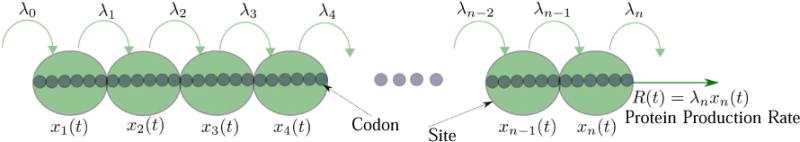
The RFM models a chain of n sites of codons (or groups of codons). The state variable x_i(t) ∈ [0, 1] represents the normalized ribosome occupancy of site i at time t. The elongation rate from site i to site i + 1 is λ_i, with λ₀ [λ_n] denoting the initiation [exit] rate. The production rate at time t is R(t) = λ_nx_n(t).

A system where each state variable describes the amount of “material” in some compartment, and the dynamics describes the flow of material within the compartments and also with the surrounding environment is called a compartmental system [19]. Compartmental systems proved to be useful models in various biological domains including physiology, pharmacokinetics, population dynamics, and epidemiology [5], [15], [18]. The RFM is clearly a nonlinear compartmental system, with x_i denoting the normalized amount of “material” in compartment i, and the flow follows a “soft” simple exclusion principle. The controllability of linear compartmental system has been addressed in several papers [20], [14].

Let x(t, a) denote the solution of (3) at time t ≥ 0 for the initial condition x(0) = a. Since the state-variables correspond to normalized occupancy levels, we always assume that a belongs to the closed n-dimensional unit cube:

$$C^n:=\{x\in {ℝ}^n:x_i\in [0,1],i=1,\dots ,n\}.$$

It has been shown in [27] that if a ∈ Cⁿ then x(t, a) ∈ Cⁿ for all t ≥ 0, that is, Cⁿ is an invariant set of the dynamics. Let int(Cⁿ) denote the interior of Cⁿ, and let ∂Cⁿ denote the boundary of Cⁿ. Ref. [27] has also shown that the RFM is a tridiagonal cooperative dynamical system [47], and that (3) admits a unique steady-state point e(λ₀, …, λ_n) ∈ int(Cⁿ) that is globally asymptotically stable, that is, lim_t→∞ x(t, a) = e for all a ∈ Cⁿ (see also [26]). This means that the ribosome density profile always converges to a steady-state profile that depends on the rates, but not on the initial condition. In particular, the production rate R(t) = λ_nx_n(t) converges to a steady-state value:

$$R:={\mathrm{\lambda }}_n{e}_n.$$ (5)

At steady-state (i.e, for x = e), the left-hand side of all the equations in (3) is zero, so

$${\mathrm{\lambda }}_0(1-e_1)={\mathrm{\lambda }}_1{e}_1(1-e_2)={\mathrm{\lambda }}_2{e}_2(1-e_3)⋮={\mathrm{\lambda }}_{n-1}{e}_{n-1}(1-e_n)={\mathrm{\lambda }}_n{e}_n=R.$$ (6)

This yields

$$\begin{array}{cc}R={\mathrm{\lambda }}_i{e}_i(1-e_{i+1}),& i=0,\dots ,n,\end{array}$$ (7)

where e₀:= 1 and e_n+1:= 0.

Remark 1

One may view (6) as a mapping from the rates [λ₀, …, λ_n]′ to the steady-state density profile and production rate [e₁ … e_n R]′. For the purposes of this paper, it is important to note that this mapping is invertible. Indeed, Eq. (7) implies that given a desired steady-state density profile and production rate [e₁ … e_n R]′ ∈ (0, 1)ⁿ × ℝ₊₊ one can immediately determine the transition rates that yield this profile, namely,

$$\begin{array}{cc}{\mathrm{\lambda }}_i=\frac{R}{e_i(1-e_{i+1})},& i=0,\dots ,n,\end{array}$$ (8)

where e₀:= 1, and e_n+1:= 0.

Note that (8) implies that λ_i increases with R and e_i+1, and decreases with e_i. This is intuitive, as a larger λ_i implies larger rate of ribosomes flow from site i to site i + 1, as well as an increase in the steady-state production rate [33]. Thus, given a desired profile with larger R and e_i+1, and a smaller e_i, the required transition rates include a larger value for λ_i.

From a biophysical point of view, this means that if there are no constraints on the transition rates then we can engineer any desired density profile together with a desired production rate. This is not trivial since in the RFM (and any other reasonable translation model) each of the state variables is affected by all the transition rates. In addition to applications in functional genomics and molecular evolution, the observation in Remark 1 is also related to problems in synthetic biology where the goal is to re-engineer the mRNA molecule so as to obtain a desired density profile and production rate (see Fig. 2).

Fig. 2.

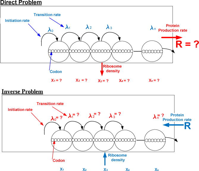
Upper part: Previous studies considered the direct problem: given the RFM parameters, i.e. the set of transition rates, λ_i, analyze the dynamics of the RFM ribosome densities x_i, and the production rate R. Lower part: here we consider the inverse problem: given a desired profile of ribosomal densities x_i, i = 1, …, n, and a desired production rate R, find the set of transition rates λ_i that steer the dynamics to this profile.

For more on the analysis of the RFM using tools from systems and control theory, see [54], [33], [34], [28], [38]. The RFM models translation on a single isolated mRNA molecule. A network of RFMs, interconnected through a common pool of “free” ribosomes has been used to model simultaneous translation of several mRNA molecules while competing for the available ribosomes [37] (see also [1] for some related ideas).

In this paper, we analyze the regulation of translation using the RFM. To do this, we first introduce two generalizations of the RFM into a control system.

A. The Controlled RFM

1) State- and Output-Controllability: Assume that all the rates λ₀, …, λ_n can be controlled. Thus, we replace every λ_i in the RFM by a function u_i(t): ℝ₊ → ℝ₊. The set of admissible controls $𝕌$ includes all the functions that are measurable, bounded and take non-negative values for all t ≥ 0. In the context of translation, controlling the u_i(t)s corresponds to dynamically varying translation factors that regulate the initiation, elongation, and exit rates along the mRNA molecule.

The problem we consider is whether it is possible, using the n + 1 control functions, to steer x and R from any initial condition to any desired conditions x^f ∈ int(Cⁿ) and R^f ∈ ℝ₊₊ in finite time.

Of course, independently controlling all the transition rates may be difficult to do in practice, so we also consider another controlled version of the RFM.

B. Output Controllability

Pick i ∈ {0, …, n}. Replace the single rate λ_i(t) by a scalar non-negative control function u(t). This models the case where a single transition rate can be controlled. In this case, we are interested in using u(t) to steer only the production rate R to a desired value R^f in finite time.

The problem we consider is whether it is possible to steer R from any initial condition to any feasible value. Of course, the set of feasible values is determined by the other, fixed, transition rates.

We show that both control problems described above are controllable. In other words, the control authority is always powerful enough to obtain any feasible desired density profile and/or production rate. This is a primarily theoretical result. However, we also show that there exist constant controls that asymptotically steer the controlled RFM to the desired densities/production rate. In the problem of controlling all the rates, these constant values are given in a simple and closed-form expression. In the second control problem, this constant value can be easily found numerically using a simple line search.

Our results are biologically relevant in several important applications. First, the problem we study, namely controlling the entire ribosomal profile using the transition rates, seems to be a fundamental problem in synthetic biology, and our results suggest that it can be addressed using a combination of mathematical, computational, and experimental approaches. Our results also provide an initial but explicit solution to this problem. While the model and problems may be relatively simple, they may provide a reasonable approximation to the biological solution in some cases. They may also be used as a starting point for addressing and solving similar problems in more comprehensive models of translation.

The next section describes our main results. Readers who are not familiar with controllability analysis may consult Appendix A for a quick review of this topic.

III. Main Results

As noted above, we consider two control problems for the RFM. We now describe their exact mathematical formulation.

A. State- and Output-Controllability

Let Ω:= Cⁿ × ℝ₊. Assume first that all the n + 1 transition rates can be controlled. The control is then u(t) = [u₀(t), …, u_n(t)]′ and the dynamics of the controlled RFM with output R(t) is described by:

$$\begin{array}{cc}{\dot{x}}_i(t)=u_{i-1}(t)x_{i-1}(t)(1-x_i(t))-u_i(t)x_i(t)(1-x_{i+1}(t)),& i=1,\dots ,n,\end{array}$$

$$R(t)=u_n(t)x_n(t).$$ (9)

We define the admissible set $𝕌$ as the set of measurable and bounded controls taking values in ${ℝ}_{+}^{n+1}$ for all time t.

Problem 1

Given arbitrary x^s, x^f ∈ int(Cⁿ) and R^s, R^f ∈ ℝ₊₊, does there always exist a time T ≥ 0 and a control $u\in 𝕌$ such that x(T, u, x^s) = x^f and R(T, u, R^s) = R^f?

Our first main result shows that the answer to this question is yes.

Theorem 1

The controlled RFM (9) is state- and output-controllable on int(Ω).

This means that the control is “powerful” enough to steer the system, in finite time, from any initial augmented profile to any desired final.

However, Theorem 1 is mainly of theoretical interest, as it does not entail a description of the required control. The next result provides a simple closed-form solution for a control that asymptotically steers the system to x^f and R^f from any initial condition. In other words, it practically solves the control synthesis problem.

Proposition 1

Fix an arbitrary $x^f={\left[x_1^f\dots x_n^f\right]}^{\prime }\in \text{int}(C^n)$ and R^f ∈ ℝ₊₊. Define $v\in {ℝ}_{++}^{n+1}$ by

$$\begin{array}{cc}{v}_i:=\frac{R^f}{x_i^f(1-x_{i+1}^f)},& i=0,\dots ,n,\end{array}$$ (10)

where $x_0^f:=1$ and $x_{n+1}^f:=0$. Then for any x^s ∈ Cⁿ and any R^s ∈ ℝ₊ applying the constant control u(t) ≡ v in (9) yields

$$\begin{array}{cc}\underset{t\to \text{∞}}{\text{lim}}x(t,u,x^s)=x^f,& \underset{t\to \text{∞}}{\text{lim}}R(t,u,R^s)=R^f\end{array}.$$ (11)

This means that the controlled RFM (9) is asymptotically state- and output-controllable on int(Ω). An important property of v is that it does not depend on x^s nor R^s, but only on the desired profile x^f and R^f. This is important as measuring x^s, that is, the initial ribosomal profile along the mRNA, may be difficult due to the current limitations in measuring ribosome densities (see, for example, [7], [9], [11]).

The proof of Proposition 1 follows immediately from Remark 1. Indeed, using the constant control u(t) ≡ v amounts to setting the desired density profile x^f as the steady-state densities of the dynamics, and R^f as the steady-state production rate. Since this steady-state is globally asymptotically stable on int(Ω), this implies (11). ■

It is important to emphasize the difference between Theorem 1 and Proposition 1. The first result guarantees the ability of steering the density profile and production rate to the desired values in finite time, but does not provide an explicit control. Proposition 1 provides an explicit, closed-form expression for fixed controls that achieve the desired goal, but only asymptotically.

Example 1

Consider the controlled RFM with dimension n = 5. Suppose that we would like to steer the ribosomal density profile along the mRNA molecule to [0.8 0.1 0.1 0.1 0.1]′, and the production rate to 1.5. The profile here is motivated by the fact that low ribosome abundance after the ORF reduces ribosome “traffic jams” that may lead to ribosome drop off. Setting x^f = [0.8 0.1 0.1 0.1 0.1]′, R^f = 1.5, and applying (10) yields

$$v={[30/425/1250/350/350/315]}^{\prime }.$$

Fig. 3 depicts the error |x(t, u, x^s) − x^f)|₁ + |R(t, u, R^s) − R^f|₁ (where |z|₁ denotes the L₁ norm of the vector z) for the initial conditions x^s = [0.5 0.5 0.5 0.5 0.5]′, R^s = 0.5, and the control u(t) ≡ v. It may be observed that the error decays at an exponential rate to zero. Thus, this control steers the system arbitrarily close to the desired final density profile x^f and production rate R^f. □

Fig. 3.

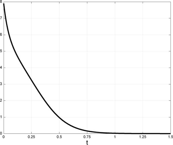
The error |x(t) − x^f)|₁ + |R(t) − R^f |₁ as a function of t.

Example 1 suggests that even though Proposition 1 provides only an asymptotic solution, the given fixed controls provide a good practical solution.

B. Output Controllability

Pick i ∈ {0, 1, …, n} and c > 0. Fix arbitrary values for the rates λ_j > 0, j ≠ i, and assume that we can control the single transition rate λ_i within the range [0, c]. This means that λ_i is replaced by a time-varying control u_i, and the set of admissible controls $𝕌$ is the set of measurable scalar functions taking values in [0, c] for all t ≥ 0. This problem represents a more realistic scenario, as we do not assume that we can control all the translation rates along the mRNA, and also the allowed control action is bounded by the value c.

In this case, we are controlling a single variable and thus we do not aim to regulate the entire ribosomal density, but only the production rate R(t), i.e. we are regulating the output. Of course, not every value of R(t) is possible, because of the other, fixed transition rates. One can in principle define the reachable set of R(t) based on the fact that the state trajectories evolve on Cⁿ. For example, if i ≠ n then R(t) = λ_nx_n(t) implies that one can define the reachable set as [0, λ_n]. However, this definition is not really relevant. Indeed, assume that some rate λ_k is much smaller than all the other rates and also much smaller than c. Then regardless of the specific control used it is clear that after some time R(t) will also be small, as λ_k will be the limiting factor, and so after some time it will become impossible to steer the production rate to every desired value in the set [0, λ_n].

We define a more meaningful reachable set for the production rate as follows. For every time T ≥ 0 and every initial condition x₀ ∈ Cⁿ, let Ωⁱ(T, x₀) ⊂ ℝ₊ denote the set of production rates that can be attained at some time t ≥ T with x(0) = x₀. Define the large-time reachable set of R as

$${\mathrm{\Omega }}^i(x_0):={\cap }_{T\ge 0}{\mathrm{\Omega }}^i(T,x_0).$$

Although the RFM is a nonlinear model, this set can be characterized explicitly.

Proposition 2

For ℓ₀, …, ℓ_n > 0 define a (n + 2) × (n + 2) symmetric, tridiagonal, and componentwise nonnegative matrix A = A(ℓ₀, …, ℓ_n) by

$$A:=\left[\begin{array}{ccccccc}0& {\text{ℓ}}_0^{-1/2}& 0& 0& \dots & 0& 0\\ {\text{ℓ}}_0^{-1/2}& 0& {\text{ℓ}}_1^{-1/2}& 0& \dots & 0& 0\\ 0& {\text{ℓ}}_1^{-1/2}& 0& {\text{ℓ}}_2^{-1/2}& \dots & 0& 0\\ & & & ⋮& & & \\ 0& 0& 0& \dots & {\text{ℓ}}_{n-1}^{-1/2}& 0& {\text{ℓ}}_n^{-1/2}\\ 0& 0& 0& \dots & 0& {\text{ℓ}}_n^{-1/2}& 0\end{array}\right]$$ (12)

Let ζ_MAX(A) denote the maximal eigenvalue of A.¹ Then for any x₀ ∈ Cⁿ,

$${\mathrm{\Omega }}^i=[0,M],$$ (13)

where M:= (ζ_MAX(A(λ₀, …, λ_i−1, c, λ_i+1, …, λ_n)))⁻².

Note that (13) implies that Ωⁱ does not depend on x₀, but only on the parameters λ_j, j ≠ i, and the value c.

Remark 2

Consider the case c → ∞. Then c^−1/2 → 0, so the largest eigenvalue of A(λ₀, …, λ_i−1, c, λ_i+1, …, λ_n) tends to

$$\text{max}\{{\zeta }_{\mathit{MAX}}(A({\mathrm{\lambda }}_0,\dots ,{\mathrm{\lambda }}_{i-1})),{\zeta }_{\mathit{MAX}}(A({\mathrm{\lambda }}_{i+1},\dots ,{\mathrm{\lambda }}_n))\},$$

so

$$M=min\{{({\zeta }_{\mathit{MAX}}(A({\mathrm{\lambda }}_0,\dots ,{\mathrm{\lambda }}_{i-1})))}^{-2},{({\zeta }_{\mathit{MAX}}(A({\mathrm{\lambda }}_{i+1},\dots ,{\mathrm{\lambda }}_n)))}^{-2}\}.$$ (14)

In other words, when the transition rate from site i to site i + 1 goes to infinity the maximal possible steady-state production rate will be the minimum of two steady-state production rates: the first [second] in an RFM of length i − 1 [n − i − 1] and parameters λ₀, …, λ_i−1 [λ_i+1, …, λ_n]. This demonstrates how in this case the other, fixed rates, being the limiting factors, determine the feasible set for the production rate.

From the biological point of view this means that if the transition rate along some region of the mRNA is very high (and thus not rate limiting) the production rate will depend only on the transition rates before and after this region, as these include the rate limiting factor. Also, the large-time reachable set for the production rate will be constrained by the rate limiting transition rates.

Example 2

Consider a controlled RFM with length n = 3, rates

$${\mathrm{\lambda }}_0=1,{\mathrm{\lambda }}_1=2,{\mathrm{\lambda }}_3=3,$$ (15)

and control u(t) = λ₂(t). Suppose that the admissible set $𝕌$ is the set of functions taking values in [0, c], with c = 15. Fig. 4 depicts (ζ_MAX(A(1, 2, λ₂, 3))⁻², for λ₂ ∈ [0, 15]. It may be seen that this is a strictly increasing function of λ₂. A calculation yields (all numbers are to four digit accuracy) (ζ_MAX (A(1, 2, 15, 3)))⁻² = 0.6538, so Ω² = [0, 0.6538].

Fig. 4.

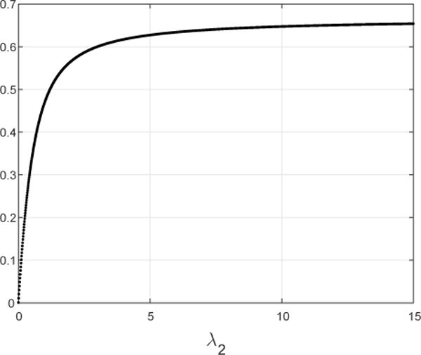
Maximal steady-state production rate (ζ_MAX(A(1, 2, λ₂, 3)))⁻² for λ₂ ∈ [0, 15].

Note that if we take c → ∞ then (14) yields

$$min\{{({\zeta }_{\mathit{MAX}}(\left[\begin{array}{ccc}0& 1& 0\\ 1& 0& 2^{-1/2}\\ 0& 2^{-1/2}& 0\end{array}\right]))}^{-2},{({\zeta }_{\mathit{MAX}}(\left[\begin{array}{cc}0& 3^{-1/2}\\ 3^{-1/2}& 0\end{array}\right]))}^{-2}\}=min\{2/3,3\}=2/3.$$

□

The next result analyzes the output controllability in Ωⁱ.

Proposition 3

The controlled RFM with λ_i replaced by a control u(t) is output-controllable in int(Ωⁱ). This means that regulating a single transition rate is still “powerful” enough to steer the production rate from any initial value to any desired final value R^f ∈ int(Ωⁱ) in finite time.

It follows from the proof of Proposition 2 (see Appendix B) that the controlled RFM is asymptotically controllable in Ωⁱ, even when $𝕌$ is restricted to constant controls only. Furthermore, since ζ_MAX(A(ℓ₀, …, ℓ_n)) is a strictly decreasing function of every ℓ_i, finding the constant value c that asymptotically steers the system to a desired value R^f ∈ int(Ω) can be easily solved numerically using a simple line search. The next example demonstrates this.

Example 3

Consider again the controlled RFM in Example 2. Recall that the admissible set $𝕌$ is the set of functions taking values in [0, c], with c = 15. Assume that our goal is to asymptotically steer the production rate to, say, R^f = 1/2. A simple line search shows that the corresponding value of λ₂ should be λ₂ ≈ 1.2 (in this particular case this can also be verified analytically using (14)). Indeed, (6) implies that for the rates in (15) and λ₂ = 1.2 the equilibrium point is e = [1/2 1/2 1/6]′, so R = λ₃e₃ = 1/2. Thus, the control u(t) ≡ 1.2 asymptotically steers the system output to R = 1/2. □

C. Sensitivity analysis

In practice, the applied controls are never exactly equal to the desired values and therefore it is important to understand the effect of small perturbations in the control values on the desired augmented profile. Since we are basically considering constant controls, it is enough to study the sensitivity of the steady-state density profile of the RFM to small changes in the λ_i’s. The sensitivity of the steady-state production rate R with respect to the λ_is has been studied in [34].

Proposition 4

Consider the RFM with dimension n, and let e:= [e₁ … e_n]′ denote the corresponding equilibrium point in int(Cⁿ). Pick i ∈ {0, …, n}. Then $\frac{\partial }{\partial {\mathrm{\lambda }}_i}{e}_k$ exists for all k, and

$$\frac{\partial }{\partial {\mathrm{\lambda }}_i}{e}_k<0,\mathit{for}\mathit{all}k\le i,$$

$$\frac{\partial }{\partial {\mathrm{\lambda }}_i}{e}_k>0,\mathit{for}\mathit{all}k>i.$$ (16)

Thus, increasing λ_i decreases [increases] the steady-state densities in sites 1, …, i [sites i + 1, …, n]. This is reasonable, as increasing λ_i increases the transition rate from site i to site i + 1 (see also [37] for some related considerations).

Example 4

Recall from Example 1 that for the RFM with n = 5 the control

$$u(t)\equiv [{30/425/1250/350/350/315]}^{\prime },$$

yields the steady-state augmented profile:

$${[eR]}^{\prime }={[0.80.10.10.10.11.5]}^{\prime }.$$ (17)

Let ũ(t) ≡ [30/4 25/12 (50/3) + ε 50/3 50/3 15]′, with ε:= 0.2 i.e. the same transition rates as before, but with ε added to λ₂. Using (6) shows that ũ yields the steady-state augmented profile

$${[\stackrel{\sim }{e}\stackrel{\sim }{R}]}^{\prime }={[0.79980.09890.10010.10010.10011.5013]}^{\prime }$$

(all numbers are to four digit accuracy). Comparing this to (17) shows that the steady-state values at sites 1, 2 decreased, and those at sites 3, 4, 5 increased. □

IV. DISCUSSION

Regulating the ribosomal density profile along the mRNA molecule, and not only the protein production rate, is an important problem in evolutionary biology, biotechnology, and synthetic biology because this density profile affects various fundamental intracellular processes including mRNA degradation, protein folding, ribosomal allocation and abortion, and more (see, for example, [55], [23], [13], [21], [31], [52]). It seems that there are still considerable gaps in our understanding of how the density profile is regulated, and how it can be re-engineered. In this paper, we addressed this issue by analyzing a mathematical model for ribosome flow, the RFM, using tools from systems and control theory.

Our results indicate that if we are able to control the transition rates along the different parts of the mRNA then we can steer the system to any desired ribosomal density profile. Also, controlling a single transition rate allows to steer the protein production rate to any desired value within a feasible range that is determined by the other, fixed transition rates. In both cases, using fixed rates is practically enough, and we show how these can be determined explicitly. These results are not trivial, as the occupation levels at different sites are interdependent due to the nonlinear excluded volume interactions between ribosomes.

Our results are based on the RFM that, as any mathematical model, is a simplification of (the biological) reality. For example, the RFM does not encapsulate some of the complex interactions between the transcript features and translation (see, e.g., [51], [42], [52]). Nevertheless, using the RFM allows one to pose the controllability problem in a well-structured way, and study it rigorously using tools from systems and control theory. We believe that our analytical results may lead to new biological insights and suggest novel and interesting biological experiments. For example, it has been suggested that higher ribosome density contributes to a higher mRNA half life in S. cerevisiae [13]. However, it is difficult to determine if the correlation is due to a larger abundance of ribosomes along the entire coding region or maybe only the ribosome density at the 5′ end of the coding region is relevant. It is also possible that this relation is due to a higher number of pre-initiation complexes at the 5′UTR (that contribute to a higher initiation rate). Specifically, it is possible that only higher pre-initiation density or ribosome density at the 5′ end is important since the degradation starts from this region. Both factors are expected to correlate with higher ribosome density along the entire coding region, and a natural question is how can we design an experiment that can separate between the two possible explanations?

The results reported here suggest that we can design a synthetic library (that can be studied in-vitro and/or in-vivo) with different strains that have different initiation rates, but identical ribosome densities along the coding regions, or strains with different levels of ribosome densities at the first codons (or any other segment) of the coding regions, but similar ribosome densities in the rest of the coding region. Using such libraries may help in understanding exactly which factor contributes to the higher mRNA half life.

We believe that the results reported in this study may contribute in the future towards a better understanding of the molecular evolution of translation. Since usually a change in a transition rate is related to mutation/change in the mRNA codons composition, obtaining a desired ribosomal density profile and production rate involves introducing changes in the nucleotide composition of the transcript. Thus, an important future study should combine controllability analysis with models of molecular evolution.

Other topics for further research include the following. First, from the biological point of view a relevant problem is controllability when only some of the transition rates can be controlled, and each rate can take values in a discrete set of possible values only. Indeed, the admissible rates are limited by factors such as the concentrations of initiation and elongation factors, and the biophysical properties of the ribosome, mRNA, and translation factors. In this case, it is clear that we cannot obtain any desired density profile, and an interesting problem may be to determine the rate values that yield the “best” approximation for a given desired profile. This requires a biologically relevant definition of this best approximation, i.e., a measure of distance between two profiles that is biologically relevant.

Second, as noted above, the RFM is the mean-field approximation of TASEP. Our results naturally raise the question of whether TASEP is controllable (in some stochastic sense). It is also interesting to examine if the analytical results obtained for the RFM can be used to synthesize suitable hopping rates for the stochastic TASEP model. In other words, suppose that we are given a desired profile P for the RFM, and determine the corresponding constant rates v_is using (10). Does using these rates (perhaps after some normalization) as the TASEP hopping rates yield the steady-state profile P in TASEP as well?

Finally, TASEP has been used to model and analyze many other applications, for example, traffic flow. The RFM can also be used to study these applications, and controllability may be important here as well. For example, a natural question is can the density along a traffic lane be steered to any arbitrary profile by regulating speed signs along different sections of the lane?

APPENDIX A: review of controllability

Controllability is a fundamental property of control systems, but it is not necessarily well-known outside of the systems and control community. For the sake of completeness, we briefly review this topic here. For more details, see e.g. [48].

Consider the control system

$$\dot{x}=f(x,u),$$

$$y=h(x,u),$$ (18)

where x: ℝ₊ → ℝⁿ is the state vector, u: ℝ₊ → ℝ^m is the control, and y: ℝ₊ → ℝ^k is the output. Let $𝕌$ denote the set of admissible controls. Assume that the trajectories of this system evolve on a state space Ω ⊆ ℝⁿ. Given an initial condition a ∈ Ω and a desired final condition b ∈ Ω, a natural control problem is: find a time T ≥ 0, and an admissible control u: [0, T] → ℝ^m such that

$$x(T,u,a)=b.$$

In other words, u steers the system from a to b in time T. Of course, such a control may not always exist. This leads to the following definition.

Definition 1

System (18) is said to be state-controllable on Ω if for any a, b ∈ Ω there exist a time T ≥ 0, and a control $u\in 𝕌$ such that x(T, u, a) = b.

Sometimes it is enough to steer the output to a desired condition. This leads to the following definition.

Definition 2

System (18) is said to be output-controllable on some set Ψ ⊆ ℝ^k if for any p, q ∈ Ψ there exist a time T ≥ 0, and a control $u\in 𝕌$ that steers the output from y(0) = p to y(T) = q.

Controllability is thus a theoretical property, but it is important in many applications, as it implies that the problem of determining a suitable control, i.e. the control synthesis problem, always admits a solution. From here on we focus on state-controllability. The notions for output-controlability are analogous.

Another useful notion, that is weaker than controllability, is called asymptotic controllability.

Definition 3

System (18) is said to be asymptotically state-controllable on Ω if for any a, b ∈ Ω there exists a control $u\in 𝕌$ such that

$$\underset{t\to \text{∞}}{\text{lim}}x(t,u,a)=b.$$

Note that this implies that for any neighborhood V of b, there exists a time T_s ≥ 0, and a control $u_s\in 𝕌$ such that x(T_s, u_s, a) ∈ V.

For nonlinear control systems, analyzing controllability or asymptotic controllability is not trivial. There exists a weaker theoretical notion that can be analyzed effectively using Lie-algebraic techniques. For a ∈ Ω, define the reachable set from a by

$$RS(a):=\{x(t,u,a):t\ge 0,u\in 𝕌\}.$$

In other words, RS(a) is the set of all states that can be reached at some time t ≥ 0 starting from x(0) = a. The system (18) is said to be accessible from a if the set RS(a) has a non empty interior. In other words, the control is powerful enough to allow steering the trajectories emanating from a to a “full set” of directions.

Example 5

Consider the scalar system $\dot{x}=u$, with Ω = ℝ. Let $𝕌$ be the set of measurable functions taking non negative values for all time t. Pick a ∈ Ω. Then RS(a) = [a, ∞), so the systen is accessible from a. However, the system is not controllable on Ω, as there does not exist any control $u\in 𝕌$ that steers a to a point b with b < a. □

Our results for the controlled RFM are based on showing that it is asymptotically state-controllable, using constant controls, and combining this with a Lie-algebraic sufficient condition for accessibility to deduce state-controllability.

To describe a sufficient condition for accessibility, consider the control affine system:

$$\dot{x}=f\left(x\right)+{\displaystyle \sum _{i=1}^m{g}_i\left(x\right)u_i},$$ (19)

and assume that $0\in 𝕌$. For two vector fields f, g: ℝⁿ → ℝⁿ, $\text{let}[f,g]:=\frac{\partial g}{\partial x}f-\frac{\partial f}{\partial x}g$. This is another vector field called the Lie-bracket of f and g. For example, if f(x) = Ax and g(x) = Bx then [f, g](x) = (BA−AB)x. It is useful to introduce a notation for iterated Lie brackets. These can be defined inductively by letting ${\text{ad}}_f^{0}g:=g$, ${\text{ad}}_f^{1}g:=\left[f,g\right]$, and ${\text{ad}}_f^{k}g:=\left[f,a{d}_f^{k-1}g\right]$ for any integer k ≥ 1.

The Lie algebra A_LA associated with (19) is the linear subspace that is generated by {f, g₁,…, g_m} and is closed under the Lie bracket operation. Let

$$A_{LA}\left(x_0\right):=\left\{p\left(x_0\right):p\in A_{LA}\right\}.$$

Roughly speaking, it can be shown that if small-time solutions of (19) emanating from a point x₀ and corresponding to piecewise constant controls “cover” a k-dimensional set, with k ≤ n, then A_LA(x₀) = ℝ^k. This yields the following sufficient condition for accessibility.

Theorem 2

If A_LA(x₀) = ℝⁿ at some point x₀ then (19) is accessible from x₀.

The next result applies Theorem 2 to analyze accessibility in the RFM when either the entry rate or exit rate is replaced by a control.

Fact 1

Consider the n-dimensional RFM with a single rate λ_i replaced by a scalar control u(t). If i = 0 or i = n then the control system is accessible from any point x ∈ int(Cⁿ).

Proof of Fact 1. Consider the controlled RFM obtained by replacing λ₀ by u(t), leaving the other rates as strictly positive constants. Let z₀(x):= λ₀(1 − x₁), z_j(x):= λ_jx_j(1 − x_j+1), for j = 1,…, n − 1, and z_n(x):= λ_nx_n. The controlled RFM satisfies:

$$\dot{x}=f\left(x\right)+g\left(x\right)u,$$ (20)

where f:= [−z₁ z₁ − z₂ z₂ – z_{3 …} z_n−1 – z_n]′, and g:= [1 − x₁ 0 _… 0]′. Let $p^k\left(x\right):=\left({\text{ad}}_f^{k}g\right)\left(x\right)$. A calculation shows that for all k ∈ {0,…, n − 1},

$$p^k={\left[p_1^k\dots p_k^k{p}_{k+1}^{k}0\dots 0\right]}^{\prime },$$

with $p_{k+1}^k={\left(-1\right)}^k{\displaystyle {\prod }_{j=1}^{k+1}\left(1-x_j\right)}{\displaystyle {\prod }_{\text{ℓ}=1}^k{\mathrm{\lambda }}_{\text{ℓ}}}$. Note that $p_{k+1}^k\ne 0$ for all x ∈ int(Cⁿ), so the n vector fields p⁰,…, pⁿ⁻¹ are linearly independent, and thus span ℝⁿ. Thus, the controlled RFM is accessible from any x ∈ int(Cⁿ).

Now consider the case where λ_n is replaced by a control u(t). For j = 1,…, n, let q_j(t):= 1 − x_n+1−j(t). Then

$$\begin{array}{l}{\dot{q}}_1=\left(1-q_1\right)u-{\mathrm{\lambda }}_{n-1}{q}_1\left(1-q_2\right),\\ {\dot{q}}_2={\mathrm{\lambda }}_{n-1q1}\left(1-q_2\right)-{\mathrm{\lambda }}_{n-2q2}\left(1-q_3\right),\\ ⋮\\ {\dot{q}}_n={\mathrm{\lambda }}_{1qn-1}\left(1-q_n\right)-{\mathrm{\lambda }}_{0qn}.\end{array}$$

This is a controlled RFM with the initiation rate replaced by a control u(t). It follows from the analysis above that this control system is accessible in int(Cⁿ), and this completes the proof. ■

Another sufficient condition for accessibility is based on linearizing the control system around an equilibrium point. For our purposes, it is enough to state this condition for the control affine system (19) with m = 1, i.e. the system:

$$\dot{x}=f\left(x\right)+g\left(x\right)u.$$ (21)

Theorem 3

[48, Ch. 3] Suppose that f(e) = 0 and that 0 ∈ int $𝕌$. Consider the linear control system

$$\dot{z}=Az+ub,$$

where $A:=\frac{\partial f}{\partial x}\left(e\right)$ and b:= g(e). If the n×n matrix [b Ab …Aⁿ⁻¹b] has rank n then (21) is accessible from some neighborhood of e.²

Example 6

Consider the RFM with n = 2, i.e.

$$\dot{x}={\mathrm{\lambda }}_0\left(1-x_1\right)-{\mathrm{\lambda }}_1{x}_1\left(1-x_2\right),$$

$$\dot{x}={\mathrm{\lambda }}_1{x}_1\left(1-x_2\right)-{\mathrm{\lambda }}_2{x}_2,$$ (22)

with λ_i > 0. The equilibrium point e of this system satisfies λ₀(1 − e₁) = λ₁e₁(1 − e₂) = λ₂e₂. Suppose now that we can control the transition rate from site 1 to site 2. To study state-controllability in the neighborhood of e, consider the control system

$${\dot{x}}_1={\mathrm{\lambda }}_0\left(1-x_1\right)-\left({\mathrm{\lambda }}_1+u\right)x_1\left(1-x_2\right),$$

$${\dot{x}}_2=\left({\mathrm{\lambda }}_1+u\right)x_1\left(1-x_2\right)-{\mathrm{\lambda }}_2{x}_2,$$ (23)

where $𝕌$ is the set of measurable functions taking values in [−ε, ε] for some sufficiently small ε > 0. This system is in the form (21) with f(x) = [λ₀(1−x₁) − λ₁x₁(1 − x₂) λ₁x₁(1 − x₂) − λ₂x₂]′, and g(x) = x₁(1−x₂) [−1 1]′. Note that f(e) = 0. To apply Theorem 3, calculate $A=\left[\begin{array}{cc}-{\mathrm{\lambda }}_0-{\mathrm{\lambda }}_1\left(1-e_2\right)& {\mathrm{\lambda }}_1{e}_1\\ {\mathrm{\lambda }}_1\left(1-e_2\right)& -{\mathrm{\lambda }}_1{e}_1-{\mathrm{\lambda }}_2\end{array}\right]$, b = e₁(1 − e₂) [−1 1]′ and

$$\left[bAb\right]=e_1\left(1-e_2\right)\left[\begin{array}{c}-1{\mathrm{\lambda }}_0+{\mathrm{\lambda }}_1\left(1-e_2\right)+{\mathrm{\lambda }}_1{e}_1\\ 1-{\mathrm{\lambda }}_1\left(1-e_2\right)-{\mathrm{\lambda }}_1{e}_1-{\mathrm{\lambda }}_2\end{array}\right].$$

Note that det $\left(\left[bAb\right]\right)=e_1^2{\left(1-e_2\right)}^2\left({\mathrm{\lambda }}_2-{\mathrm{\lambda }}_0\right)$. Since e ∈ int(C²), Theorem 3 implies that if λ₀ ≠ λ₂ then (23) is accessible in a neighborhood of e.

Now consider (23) with λ₀ = λ₂. Then z:= x₁ + x₂ satisfies

$$\dot{z}={\mathrm{\lambda }}_0\left(1-z\right).$$

Thus, any trajectory with x₁(0) + x₂(0) = 1 satisfies x₁(t) + x₂(t) ≡ 1 for any control u, and this implies that in this case (23) is not accessible and not state-controllable on C². Summarizing, in this case the condition in Theorem 3 allows us to completely analyze the accessibility of (23). □

This example may suggest that accessibility is lost when one of the internal (or elongation) rates λ_i, i ∈ {1, …, n − 1}, is replaced by a control, at least for some values of the other rates. However, the next example shows that is not necessarily true.

Example 7

Consider the RFM with n = 3, i.e.

$${\dot{x}}_1={\mathrm{\lambda }}_0\left(1-x_1\right)-{\mathrm{\lambda }}_1{x}_1\left(1-x_2\right),$$

$${\dot{x}}_2={\mathrm{\lambda }}_1{x}_1\left(1-x_2\right)-{\mathrm{\lambda }}_2{x}_2\left(1-x_3\right),$$

$${\dot{x}}_2={\mathrm{\lambda }}_2{x}_2\left(1-x_3\right)-{\mathrm{\lambda }}_3{x}_3,$$

with λ_i > 0. Suppose that we can control the transition rate from site 1 to site 2, so we consider the control system:

$${\dot{x}}_1={\mathrm{\lambda }}_0\left(1-x_1\right)-x_1\left(1-x_2\right)u,$$

$${\dot{x}}_2=x_1\left(1-x_2\right)u-{\mathrm{\lambda }}_2{x}_2\left(1-x_3\right),$$

$${\dot{x}}_2={\mathrm{\lambda }}_2{x}_2\left(1-x_3\right)-{\mathrm{\lambda }}_3{x}_3.$$ (24)

We may ignore the term x₁(1 − x₂) multiplying u, as it is strictly positive for all x ∈ int(C³). Thus, the control system is in the form (21) with f(x) = [λ₀(1 − x₁) −λ₂x₂(1 − x₃) λ₂x₂(1 − x₃) − λ₃x₃]′, and g(x) = [−1 1 0]′. A calculation yields

$$v^1:=\left[f,g\right]={\left[-{\mathrm{\lambda }}_0{\mathrm{\lambda }}_2\left(1-x_3\right)-{\mathrm{\lambda }}_2\left(1-x_3\right)\right]}^{\prime },$$

$$v^2:=\left[\left[f,\left[f,g\right]\right],\left[f,g\right]\right]={\left[0{\mathrm{\lambda }}_2^2\left({\mathrm{\lambda }}_3\left(2-x_3\right)-{\mathrm{\lambda }}_2{\left(1-x_3\right)}^2\right){\mathrm{\lambda }}_2^2\left({\mathrm{\lambda }}_2{\left(1-x_3\right)}^2-{\mathrm{\lambda }}_3\right)\right]}^{\prime },$$

and

$$v^3:=\left[v^2,v^1\right]={\left[0{\mathrm{\lambda }}_2^3\left({\mathrm{\lambda }}_3{x}_3+{\mathrm{\lambda }}_2{\left(1-x_3\right)}^2\right)-{\mathrm{\lambda }}_2^3\left({\mathrm{\lambda }}_2{\left(1-x_3\right)}^2+{\mathrm{\lambda }}_3\right)\right]}^{\prime },$$

so

$$\text{det}\left(\left[v^1{v}^2{v}^3\right]\right)=2{\mathrm{\lambda }}_0{\mathrm{\lambda }}_2^5{\mathrm{\lambda }}_3^2\left(1-x_3\right).$$

Since this is different from zero for all x ∈ int(C³), we conclude that (24) is accessible from every x ∈ int(C³). □

Appendix B: Proofs

Proof of Theorem 1. We begin by defining a new control system obtained by replacing λ_i, i ∈ {0, …, n−1}, in the RFM (3) by a control function u_i(t): ℝ₊ → ℝ₊ (but leaving λ_n as a constant rate). This yields

$$\dot{x}=g_0(x)+{\displaystyle \sum _{i=1}^n{u}_{i-1}{g}_i}(x),$$ (25)

where g₀(x):= [0 … 0 – λ_nx_n]′, g₁(x):= [1 –x₁ 0 … 0]′, and for any j ≥ 2, g_j(x) contains the value −x_j−1(1 − x_j) in its (j − 1)’th coordinate, the value x_j−1(1 − x_j) in its j’th coordinate, and the value 0 otherwise. For example, for n = 4:

$$g_0(x)={\left[\begin{array}{cccc}0& 0& 0& -{\mathrm{\lambda }}_4{x}_4\end{array}\right]}^{\prime },$$

$$g_1(x)={\left[\begin{array}{cccc}1-x_1& 0& 0& 0\end{array}\right]}^{\prime },$$

$$g_2(x)={\left[\begin{array}{cccc}-x_1(1-x_2)& x_1(1-x_2)& 0& 0\end{array}\right]}^{\prime },$$

$$g_3(x)={\left[\begin{array}{cccc}0& -x_2(1-x_3)& x_2(1-x_3)& 0\end{array}\right]}^{\prime },$$

$$g_4(x)={\left[\begin{array}{cccc}0& 0& -x_3(1-x_4)& x_3(1-x_4)\end{array}\right]}^{\prime }.$$

Pick x^f ∈ int(Cⁿ) and z ∈ ℝⁿ. Then it is straightforward to show that

$$z={\displaystyle \sum _{i=1}^n{\alpha }_i{g}_i(x^f),}$$

where

$${\alpha }_i:=\frac{{\sum }_{k=i}^n{z}_k}{x_{i-1}^f(1-x_i^f)},$$

with $x_0^f:=1$. Note that since x^f ∈ int(Cⁿ), α_i is well-defined for all i = 1,…,n. We conclude that the vector fields g₁(x^f),…, g_n(x^f) span ℝⁿ. This implies, by known accessibility results (see, e.g. [48, Ch. 4]), that there exists a set V = V (x^f) ⊆ int(Cⁿ), that has a nonempty interior in ℝⁿ, and such that every p ∈ V can be steered to x^f in finite time. Fix arbitrary q ∈ int(V) and x^s ∈ Cⁿ. By Proposition 1, there exist constant controls u₀, …, u_n−1 such that lim_t→∞ x(t, u, x^s) = q. Therefore there exists a time τ > 0 such that x(τ, u, x^s) ∈ V. The control u(t), t ∈ [0, τ], can now be time-concatenated to a control w that steers x(τ, u, x^s) to x^f. Up to now, we only used u = [u₀ … u_n−1]′ (with λ_n > 0 fixed) and found a control u that steers x(0) = x^s to x(T) = x^f. In particular, this control steers $x_n(0)=x_n^s$ to $x_n(T)=x_n^f$. Now replace λ_n by a control u_n, and set $u_n(t)\equiv \frac{R^f}{x_n^f}$. Then R(T) = u_n(T)x_n(T) =R^f, and this completes the proof.

Remark 3

Note that the construction above may lead to a production rate R(t) that is discontinuous at t = 0. This can be easily overcome using any control u_n(t) that smoothly interpolates between the values $u_n(0):=\frac{R^s}{x_n^s}$ and $u_n(T):=\frac{R^f}{x_n^f}$. For example, u_n(t) could be picked linear in t. Also, we can take $u_n(t)\equiv \frac{R^s}{x_n^s}$ for t ∈ [0, T − ε] and then a smooth interpolation between this value and $\frac{R^f}{x_n^f}$on t ∈ [T − ε, T]. This way u_i(t) is constant on [0, T − ε] for all i = 1, …, n.

Proof of Proposition 2. Consider the RFM with rates λ₀, …, λ_n. It was shown in [33, Proposition 1] that R is a strictly increasing function of every λ_i. This means that in order to analyze Ωⁱ in the controlled RFM with $u\in 𝕌$ it is enough to consider the reachable set for the controls u(t) ≡ 0 and u(t) ≡ c. It has been shown in [33] that for the rates λ₀, …, λ_n, the steady state production rate is R = (ζ_MAX(A(λ₀, …, λ_n)))⁻²ⁿ. Thus for the two controls above R(t) in the controlled RFM converges to 0 and to M:= (ζ_MAX (A(λ₀, …, λ_i−1, c, λ_i, …, λ_n)))⁻², respectively. We conclude that Ωⁱ = [0, M]. ■

Proof of Proposition 3. Pick R^f ∈ int(Ωⁱ). Our goal is to show that there exist a finite time T ≥ 0 and a control $u\in 𝕌$ that steers R(t) to R^f in time T. We consider two cases.

Case 1. Suppose that i ≠ n. Since R^f ∈ int(Ωⁱ), there exists ε > 0 such that (R^f − ε) ∈ Ωⁱ and (R^f + ε) ∈ Ωⁱ. Therefore, there exist v⁻, v⁺ ∈ [0, c] such that for the control u⁻(t) ≡ v⁻ [u⁺(t) ≡ v⁺] the production rate converges to R^f − ε [R^f +ε] for any x₀. Applying u⁻ for a sufficiently long time T₁ yields R(T₁) < R^f. Now applying u⁺ for a sufficiently long time T₂ yields R(T₁ + T₂) > R^f. Since R(t) is continuous, this implies that there exists T ∈ [T₁, T₁ + T₂] such that R(T) = R^f.

Case 2. Suppose that i = n, i.e. R(t) = u(t)x_n(t). The argument used in Case 1 does not hold as is because now a discontinuity in u yields a discontinuity in R(t). However, it is clear that we can design a control u by concatenating u(t) ≡ v⁻ for t ∈ [0, T₁], then a function of time satisfying u(T₁) = v⁻ and u(T₁ + τ) = v⁺, with τ > 0, and finally u(t) ≡ v⁺ for t ≥ T₁ + τ, and that this will steer R(t) to R^f at some final time T. ■

Proof of Proposition 4. It has been shown in [33] that $\frac{\partial R}{\partial {\mathrm{\lambda }}_i}$ exists and is strictly positive for all i ∈ {0, …, n} Combining this with (6) implies that $\frac{\partial e_k}{\partial {\mathrm{\lambda }}_i}$ exists for all k ∈ {1, …, n} and all i ∈ {0, …, n}. Pick i ∈ {1, …, n − 2}. Differentiating (6) with respect to λ_i yields

$$-{\mathrm{\lambda }}_0{e}_1^{\prime }={\mathrm{\lambda }}_1{e}_1^{\prime }(1-e_2)-{\mathrm{\lambda }}_1{e}_1{e}_2^{\prime }={\mathrm{\lambda }}_2{e}_2^{\prime }(1-e_3)-{\mathrm{\lambda }}_2{e}_2{e}_3^{\prime }⋮={\mathrm{\lambda }}_{i-1}{e}_{i-1}^{\prime }(1-e_i)-{\mathrm{\lambda }}_{i-1}{e}_{i-1}{e}_i^{\prime }=e_i(1-e_{i+1})+{\mathrm{\lambda }}_i{e}_i^{\prime }(1-e_{i+1})-{\mathrm{\lambda }}_i{e}_i{e}_{i+1}^{\prime }={\mathrm{\lambda }}_{i+1}{e}_{i+1}^{\prime }(1-e_{i+2})-{\mathrm{\lambda }}_{i+1}{e}_{i+1}{e}_{i+2}^{\prime }⋮={\mathrm{\lambda }}_{n-1}{e}_{n-1}^{\prime }(1-e_n)-{\mathrm{\lambda }}_{n-1}{e}_{n-1}{e}_n^{\prime }={\mathrm{\lambda }}_n{e}_n^{\prime }=R^{\prime },$$ (26)

where we use the notation $f^{\prime }:=\frac{\partial f}{\partial {\mathrm{\lambda }}_i}$. Since R′ > 0, we conclude that $e_1^{\prime }<0$. Now the equation ${\mathrm{\lambda }}_1{e}_1^{\prime }(1-e_2)-{\mathrm{\lambda }}_1{e}_1{e}_2^{\prime }=R^{\prime }$, and the fact that e ∈ (0, 1)ⁿ yield $e_2^{\prime }<0$. Continuing in this fashion yields $e_j^{\prime }<0$ for all j ≤ i. The last equality in (26) yields ${\mathrm{\lambda }}_1{e}_n^{\prime }>0$, so $e_n^{\prime }<0$. Now the equality ${\mathrm{\lambda }}_{n-1}{e}_{n-1}^{\prime }(1-e_n)-{\mathrm{\lambda }}_{n-1}{e}_{n-1}{e}_n^{\prime }=R^{\prime }$ yields $e_{n-1}^{\prime }>0$, and continuing in this fashion yields $e_j^{\prime }>0$ for all j > i. This completes the proof for the case i ∈ {1, …, n − 2}. The proof when i ∈ {0, n − 1, n} is similar. ■

References

- 1.Algar RJR, Ellis T, Stan GB. Modelling essential interactions between synthetic genes and their chassis cell. Proc 53rd IEEE Conf on Decision and Control. 2014:5437–5444. [Google Scholar]
- 2.Arava Y, Wang Y, Storey JD, Liu CL, Brown PO, Herschlag D. Genome-wide analysis of mRNA translation profiles in Saccharomyces cerevisiae. Proceedings of the National Academy of Sciences. 2003;100(7):3889–3894. doi: 10.1073/pnas.0635171100. [DOI] [PMC free article] [PubMed] [Google Scholar]
- 3.Binnie C, Cossar JD, Stewart DI. Heterologous biopharmaceutical protein expression in Streptomyces. Trends Biotechnol. 1997;15(8):315–20. doi: 10.1016/s0167-7799(97)01062-7. [DOI] [PubMed] [Google Scholar]
- 4.Blythe RA, Evans MR. Nonequilibrium steady states of matrix-product form: a solver’s guide. J Phys A: Math Theor. 2007;40(46):R333–R441. [Google Scholar]
- 5.Brauer F. Compartmental models in epidemiology. In: Brauer F, van den Driessche P, Wu J, editors. Mathematical Epidemiology, ser Lecture Notes in Mathematics. Vol. 1945. Springer; Berlin Heidelberg: 2008. pp. 19–79. [Google Scholar]
- 6.Chu D, Zabet N, von der Haar T. A novel and versatile computational tool to model translation. Bioinformatics. 2012;28(2):292–3. doi: 10.1093/bioinformatics/btr650. [DOI] [PubMed] [Google Scholar]
- 7.Dana A, Tuller Determinants of translation elongation speed and ribosomal profiling biases in mouse embryonic stem cells. PLOS Computational Biology. 2012;8(12):e1002755. doi: 10.1371/journal.pcbi.1002755. [DOI] [PMC free article] [PubMed] [Google Scholar]
- 8.Dana A, Tuller T. Efficient manipulations of synonymous mutations for controlling translation rate–an analytical approach. J Comput Biol. 2012;19:200–231. doi: 10.1089/cmb.2011.0275. [DOI] [PubMed] [Google Scholar]
- 9.Dana A, Tuller T. Mean of the typical decoding rates: a new translation efficiency index based on ribosome analysis data. G3: Genes, Genomes, Genetics. 2014 doi: 10.1534/g3.114.015099. [DOI] [PMC free article] [PubMed] [Google Scholar]
- 10.Deneke C, Lipowsky R, Valleriani A. Effect of ribosome shielding on mRNA stability. Phys Biol. 2013;10(4) doi: 10.1088/1478-3975/10/4/046008. 046008. [DOI] [PubMed] [Google Scholar]
- 11.Diament A, Tuller T. Ribosome profiling resolution in practice. under review. 2016 [Google Scholar]
- 12.Drummond DA, Wilke CO. Mistranslation-induced protein misfolding as a dominant constraint on coding-sequence evolution. Cell. 2008;134:341–352. doi: 10.1016/j.cell.2008.05.042. [DOI] [PMC free article] [PubMed] [Google Scholar]
- 13.Edri S, Tuller T. Quantifying the effect of ribosomal density on mRNA stability. PLoS One. 2014;9:e102308. doi: 10.1371/journal.pone.0102308. [DOI] [PMC free article] [PubMed] [Google Scholar]
- 14.Hayakawa Y, Hosoe S, Hayashi M, Ito M. On the structural controllability of compartmental systems. IEEE Trans Automat Control. 1984;29(1):17–24. [Google Scholar]
- 15.Holza M, Fahrb A. Compartment modeling. Advanced Drug Delivery Reviews. 2001;48:249–264. doi: 10.1016/s0169-409x(01)00118-1. [DOI] [PubMed] [Google Scholar]
- 16.Hsieh AC, Liu Y, Edlind MP, Ingolia NT, Janes MR, Sher A, Shi EY, Stumpf CR, Christensen C, Bonham MJ, Wang S, Ren P, Martin M, Jessen K, Feldman ME, Weissman JS, Shokat KM, Rommel C, Ruggero D. The translational landscape of mTOR signalling steers cancer initiation and metastasis. Nature. 2012;485:55–61. doi: 10.1038/nature10912. [DOI] [PMC free article] [PubMed] [Google Scholar]
- 17.Jackson R, Hellen C, Pestova T. The mechanism of eukaryotic translation initiation and principles of its regulation. Nat Rev Mol Cell Biol. 2010;11(2):113–27. doi: 10.1038/nrm2838. [DOI] [PMC free article] [PubMed] [Google Scholar]
- 18.Jacquez JA. Biology and Medicine. 3rd. Ann Arbor, MI: BioMedware; 1996. Compartmental Analysis. [Google Scholar]
- 19.Jacquez JA, Simon CP. Qualitative theory of compartmental systems. SIAM Review. 1993;35(1):43–79. doi: 10.1016/s0025-5564(02)00131-1. [DOI] [PubMed] [Google Scholar]
- 20.Johnson LE. Control and controllability in compartmental systems. Mathematical Biosciences. 1976;30(1–2):181–190. [Google Scholar]
- 21.Kimchi-Sarfaty C, Oh JM, Kim IW, Sauna ZE, Calcagno AM, Ambudkar SV, Gottesman MM. A “silent” polymorphism in the MDR1 gene changes substrate specificity. Science. 2007;315:525–528. doi: 10.1126/science.1135308. [DOI] [PubMed] [Google Scholar]
- 22.Kimchi-Sarfaty C, Schiller T, Hamasaki-Katagiri N, Khan MA, Yanover C, Sauna ZE. Building better drugs: developing and regulating engineered therapeutic proteins. Trends Pharmacol Sci. 2013;34(10):534–548. doi: 10.1016/j.tips.2013.08.005. [DOI] [PubMed] [Google Scholar]
- 23.Kurland C. Translational accuracy and the fitness of bacteria. Annu Rev Genet. 1992;26:29–50. doi: 10.1146/annurev.ge.26.120192.000333. [DOI] [PubMed] [Google Scholar]
- 24.Liu Y-Y, Slotine J-J, Barabasi A-L. Controllability of complex networks. Nature. 2011;473:167–173. doi: 10.1038/nature10011. [DOI] [PubMed] [Google Scholar]
- 25.Loayza-Puch F, Drost J, Rooijers K, Lopes R, Elkon R, Agami R. p53 induces transcriptional and translational programs to suppress cell proliferation and growth. Genome Bio. 2013;14(4):1–12. doi: 10.1186/gb-2013-14-4-r32. [DOI] [PMC free article] [PubMed] [Google Scholar]
- 26.Margaliot M, Sontag ED, Tuller T. Entrainment to periodic initiation and transition rates in a computational model for gene translation. PLoS ONE. 2014;9(5):e96039. doi: 10.1371/journal.pone.0096039. [DOI] [PMC free article] [PubMed] [Google Scholar]
- 27.Margaliot M, Tuller T. Stability analysis of the ribosome flow model. IEEE/ACM Trans Computational Biology and Bioinformatics. 2012;9:1545–1552. doi: 10.1109/TCBB.2012.88. [DOI] [PubMed] [Google Scholar]
- 28.Margaliot M, Tuller T. Ribosome flow model with positive feedback. J Royal Society Interface. 2013;10:20130267. doi: 10.1098/rsif.2013.0267. [DOI] [PMC free article] [PubMed] [Google Scholar]
- 29.Moks T, Abrahmsen L, Holmgren E, Bilich M, Olsson A, Pohl G, Sterky C, Hultberg H, Josephson SA. Expression of human insulin-like growth factor I in bacteria: use of optimized gene fusion vectors to facilitate protein purification. Biochemistry. 1987;26(17):5239–44. doi: 10.1021/bi00391a005. [DOI] [PubMed] [Google Scholar]
- 30.Olshevsky A. Minimal controllability problems. IEEE Trans Control of Network Systems. 2014;1(3):249–258. [Google Scholar]
- 31.Pechmann S, Frydman J. Evolutionary conservation of codon optimality reveals hidden signatures of cotranslational folding. Nat Struct Mol Biol. 2013;20(2):237–43. doi: 10.1038/nsmb.2466. [DOI] [PMC free article] [PubMed] [Google Scholar]
- 32.Plotkin JB, Kudla G. Synonymous but not the same: the causes and consequences of codon bias. Nat Rev Genet. 2010;12:32–42. doi: 10.1038/nrg2899. [DOI] [PMC free article] [PubMed] [Google Scholar]
- 33.Poker G, Zarai Y, Margaliot M, Tuller T. Maximizing protein translation rate in the nonhomogeneous ribosome flow model: A convex optimization approach. J Royal Society Interface. 2014;11(100):20140713. doi: 10.1098/rsif.2014.0713. [DOI] [PMC free article] [PubMed] [Google Scholar]
- 34.Poker G, Margaliot M, Tuller T. Sensitivity of mRNA translation. Sci Rep. 2015;5(12795) doi: 10.1038/srep12795. [DOI] [PMC free article] [PubMed] [Google Scholar]
- 35.Proshkin S, Rahmouni A, Mironov A, Nudler E. Cooperation between translating ribosomes and RNA polymerase in transcription elongation. Science. 2010;328(5977):504–8. doi: 10.1126/science.1184939. [DOI] [PMC free article] [PubMed] [Google Scholar]
- 36.Racle J, Picard F, Girbal L, Cocaign-Bousquet M, Hatzimanikatis V. A genome-scale integration and analysis of Lactococcus lactis translation data. PLOS Computational Biology. 2013;9(10):e1003240. doi: 10.1371/journal.pcbi.1003240. [DOI] [PMC free article] [PubMed] [Google Scholar]
- 37.Raveh A, Margaliot M, Sontag ED, Tuller T. A model for competition for ribosomes in the cell. 2015 doi: 10.1098/rsif.2015.1062. submitted. [Online]. Available: http://arxiv.org/abs/1508.02408. [DOI] [PMC free article] [PubMed]
- 38.Raveh A, Zarai Y, Margaliot M, Tuller T. Ribosome flow model on a ring. IEEE/ACM Trans Computational Biology and Bioinformatics. 2015;12(6):1429–1439. doi: 10.1109/TCBB.2015.2418782. [DOI] [PubMed] [Google Scholar]
- 39.Reuveni S, Meilijson I, Kupiec M, Ruppin E, Tuller T. Genome-scale analysis of translation elongation with a ribosome flow model. PLOS Computational Biology. 2011;7:e1002127. doi: 10.1371/journal.pcbi.1002127. [DOI] [PMC free article] [PubMed] [Google Scholar]
- 40.Romanos MA, Scorer CA, Clare JJ. Foreign gene expression in yeast: a review. Yeast. 1992;8(6):423–88. doi: 10.1002/yea.320080602. [DOI] [PubMed] [Google Scholar]
- 41.Ruppin TT, Kupiec M, E Determinants of protein abundance and translation efficiency in S. cerevisiae. PLOS Computational Biology. 2007;3:2510–2519. doi: 10.1371/journal.pcbi.0030248. [DOI] [PMC free article] [PubMed] [Google Scholar]
- 42.Sabi R, Tuller T. A comparative genomics study on the effect of individual amino acids on ribosome stalling. BMC genomics. 2015 doi: 10.1186/1471-2164-16-S10-S5. [DOI] [PMC free article] [PubMed] [Google Scholar]
- 43.Salis H, Mirsky E, Voigt C. Automated design of synthetic ribosome binding sites to control protein expression. Nat Biotechnol. 2009;27(10):946–50. doi: 10.1038/nbt.1568. [DOI] [PMC free article] [PubMed] [Google Scholar]
- 44.Schadschneider A, Chowdhury D, Nishinari K. Stochastic Transport in Complex Systems: From Molecules to Vehicles. Elsevier; 2011. [Google Scholar]
- 45.Shah P, Ding Y, Niemczyk M, Kudla G, Plotkin J. Rate-limiting steps in yeast protein translation. Cell. 2013;153(7):1589–601. doi: 10.1016/j.cell.2013.05.049. [DOI] [PMC free article] [PubMed] [Google Scholar]
- 46.Shaw LB, Zia RKP, Lee KH. Totally asymmetric exclusion process with extended objects: a model for protein synthesis. Phys Rev E. 2003;68 doi: 10.1103/PhysRevE.68.021910. 021910. [DOI] [PubMed] [Google Scholar]
- 47.Smith HL. Monotone Dynamical Systems: An Introduction to the Theory of Competitive and Cooperative Systems, ser Mathematical Surveys and Monographs. Providence, RI: Amer Math Soc. 1995;41 [Google Scholar]
- 48.Sontag ED. Mathematical Control Theory: Deterministic Finite Dimensional Systems. 2nd. New York: Springer; 1998. [Google Scholar]
- 49.Sun L, Xiong Y, Bashan A, Zimmerman E, Daube SS, Peleg Y, Albeck S, Unger T, Yonath H, Krupkin M, Matzov R, Yonath A. A recombinant collagen-mRNA platform for controllable protein synthesis. Chembiochem. 2015;16(10):1415–9. doi: 10.1002/cbic.201500205. [DOI] [PMC free article] [PubMed] [Google Scholar]
- 50.Tomlinson VA, Newbery HJ, Wray NR, Jackson J, Larionov A, Miller WR, Dixon JM, Abbott CM. Translation elongation factor eEF1A2 is a potential oncoprotein that is overexpressed in two-thirds of breast tumours. BMC Cancer. 2005;5(1):1–7. doi: 10.1186/1471-2407-5-113. [DOI] [PMC free article] [PubMed] [Google Scholar]
- 51.Tuller T, Veksler I, Gazit N, Kupiec M, Ruppin E, Ziv M. Composite effects of the coding sequences determinants on the speed and density of ribosomes. Genome Biol. 2011;12(11):R110. doi: 10.1186/gb-2011-12-11-r110. [DOI] [PMC free article] [PubMed] [Google Scholar]
- 52.Tuller T, Zur H. Multiple roles of the coding sequence 5′ end in gene expression regulation. Nucleic Acids Res. 2015;43(1):13–28. doi: 10.1093/nar/gku1313. [DOI] [PMC free article] [PubMed] [Google Scholar]
- 53.Waldman YY, Tuller T, Sharan R, Ruppin E. TP53 cancerous mutations exhibit selection for translation efficiency. Cancer Res. 2009;69:8807–13. doi: 10.1158/0008-5472.CAN-09-1653. [DOI] [PubMed] [Google Scholar]
- 54.Zarai Y, Margaliot M, Tuller T. Explicit expression for the steady-state translation rate in the infinite-dimensional homogeneous ribosome flow model. IEEE/ACM Trans Computational Biology and Bioinformatics. 2013;10:1322–1328. doi: 10.1109/TCBB.2013.120. [DOI] [PubMed] [Google Scholar]
- 55.Zhang G, Hubalewska M, Ignatova Z. Transient ribosomal attenuation coordinates protein synthesis and co-translational folding. Nat Struct Mol Biol. 2009;16(3):274–80. doi: 10.1038/nsmb.1554. [DOI] [PubMed] [Google Scholar]
- 56.Zia R, Dong J, Schmittmann B. Modeling translation in protein synthesis with TASEP: A tutorial and recent developments. J Statistical Physics. 2011;144:405–428. [Google Scholar]
- 57.Zur H, Tuller T. New universal rules of eukaryotic translation initiation fidelity. PLOS Computational Biology. 2013;9(7):e1003136. doi: 10.1371/journal.pcbi.1003136. [DOI] [PMC free article] [PubMed] [Google Scholar]