Regularization Parameter Selection for Penalized-likelihood List-mode Image Reconstruction in PET

Abstract

Penalized likelihood (PL) reconstruction has demonstrated potential to improve image quality of positron emission tomography (PET) over unregularized ordered-subsets expectation-maximization (OSEM) algorithm. However, selecting proper regularization parameters in PL reconstruction has been challenging due to the lack of ground truth and variation of penalty functions. Here we present a method to choose regularization parameters using a cross-validation log-likelihood (CVLL) function. This new method does not require any knowledge of the true image and is directly applicable to list-mode PET data. We performed statistical analysis of the mean and variance of the CVLL. The results show that the CVLL provides an unbiased estimate of the log-likelihood function calculated using the noise free data. The predicted variance can be used to verify the statistical significance of the difference between CVLL values. The proposed method was validated using simulation studies and also applied to real patient data. The reconstructed images using optimum parameters selected by the proposed method show good image quality visually.

1. Introduction

Iterative image reconstruction has been widely used for positron emission tomography (PET) to improve image quality. Maximum likelihood (ML) expectation maximization (EM) algorithm and its accelerated variant ordered-subset (OS) EM (Hudson and Larkin, 1994) estimate images from projections by maximizing the log-likelihood of measured data. Generally, statistical image reconstruction can achieve higher image quality compared to filtered back projection (FBP), because it can model data noise distributions and non-ideal system responses. However, a true ML solution is usually very noisy. As a result, ML algorithm is often stopped at early iterations before convergence and post-filtering is applied in clinical applications.

Penalized likelihood (PL) image reconstruction incorporates a penalty function into the objective function to control noise. It is also known as maximum a posteriori (MAP) reconstruction in the Bayesian framework (Qi and Leahy, 2006). One or more regularization parameters are usually required to balance the relative strength between the log-likelihood function and the penalty function. Larger regularization parameter leads to smoother images but also blurs small objects and edges. The selection of optimal parameters is rather challenging since it depends not only on the penalty itself but also on the unknown images. Different penalty functions have different effects on PL image reconstruction, so a regularization parameter that is suitable for one penalty function usually does not work well for other penalty functions. One approach is to choose the regularization parameters to achieve a desired spatial resolution by theoretically analyzing the noise and resolution properties of PL reconstructions (Fessler and Rogers, 1996, Qi and Leahy, 2000). Furthermore, the penalty function can be designed to maximize the lesion detectability if prior knowledge of the lesion is available (Yang et al., 2013). However, the theoretical analysis only works for quadratic penalty functions and cannot be applied to edge-preserving regularizations.

There is also a large body of parameter selection methods that seek to minimize the total predicted mean squared error (MSE) (Thompson et al., 1991). Since the true MSE is impractical to compute, many approximate methods have been developed, including the L-curve method (Hansen and O'Leary, 1993), the χ² method, and generalized cross validation (GCV) (Thompson et al., 1991). The most attractive one is the use of Stein’s unbiased risk estimate (SURE) (Stein, 1981), which provides an unbiased estimation of the true MSE without requiring the noise-free data. SURE was originally developed for Gaussian noise. Modifications have been proposed to tackle Poisson noise in the applications of image deconvolution (Hudson and Lee, 1998, Bardsley† and Laobeul, 2008, Carlavan and Blanc-Féraud, 2012). Zanella et al (Zanella et al., 2009) also proposed a discrepancy principle for image denoising in Poisson noise. In PET, SURE has been used to select the low-pass filter for the FBP reconstruction (Pawitan and O'Sullivan, 1993). Recently, Zhou et al applied a Monte Carlo SURE-based parameter selection method to PL image reconstruction in PET (Zhou and Qi, 2014). The key component of SURE computation is the first-order derivative of the image estimator with respect to the data. Closed-form solution is generally unavailable since the PL estimator is a nonlinear function of data and is computed using an iterative algorithm. Even when a closed-form expression is available, evaluation of the Jacobian matrix often involves inversion of a huge matrix, which can be difficult to compute due to the large matrix size.

Since PET data follow a Poisson distribution, MSE based criterion is less desirable. Here we propose a cross-validation method based on the Poisson log-likelihood function. Cross validation has been proposed to select the number of iterations in ML EM algorithm for both conventional PET (Llacer et al., 1993) and dynamic PET reconstruction (Selivanov et al., 2001). In these papers, the measured data were randomly separated into two identically distributed datasets and both datasets were reconstructed using the other dataset for cross validation. The final reconstructed image is the sum of the two optimal reconstructions.

Here we use the cross validation method to select regularization parameters in PL reconstruction. We divide the events unequally, using majority of the events for reconstruction and leaving a small fraction of events out for validation. The ratio between counts for reconstruction and for cross validation will be determined based on the statistical analysis of the variance. Similar to the SURE-based parameter selection method, it does not require any knowledge of the true image, but has a much simpler form and less computational burden. We demonstrate the effectiveness of the proposed method using both simulation and real data.

The rest of this paper is organized as follows. Section 2 introduces the penalized likelihood reconstruction and the proposed cross validation method. Section 3 describes the details of the simulation setup and patient data acquisition. Reconstructed images and quantitative studies are shown in Section 4. Finally, we discuss important findings in Section 5 and draw conclusions in Section 6.

2. Methods

2.1 Penalized likelihood reconstruction

In PET image reconstruction, the measured data y can be modeled as a collection of independent Poisson random variables whose mean ȳ(x) is related to the unknown emission image x through an affine transform

$$\overline{\mathit{y}}(\mathit{x})=\mathit{\text{Px}}+\mathit{r}$$

where P = {p_i,j} ∈ ℝ^M×N denotes the probability of detecting an emission event from pixel j, j ∈ 1,…,N, at detector pair i, i ∈ 1,…,M, and r denotes the mean of background scattered and random events. The expectation of the background, r, is estimated before reconstruction, and is treated as a known vector during the reconstruction. The PL reconstruction is obtained by maximizing a penalized likelihood function

$${\hat{\mathit{x}}}_{\beta }(\mathit{y})={\text{arg max}}_{x\ge 0}\{\mathrm{L}(\mathit{y}|\mathit{x})-\beta \mathrm{U}(\mathit{x};\delta )\}$$

where L (y|x) is the Poisson log-likelihood function defined as

$$\mathrm{L}(\mathit{y}|\mathit{x})=\sum _i\{y_i\text{ ln}({(\mathit{\text{Px}}+\mathit{r})}_i)-{(\mathit{\text{Px}}+\mathit{r})}_i\}$$

and U(x; δ) is the penalty function with β and δ being the regularization parameters.

2.2 Cross validation

All penalty functions in PL reconstructions require one (β) or more (β, δ) parameters. Selecting the proper values of the regularization parameters often requires the knowledge of the true image, such as those based on the mean squared error (MSE) either in the image domain or the sinogram domain. Here we propose a parameter selection method that does not rely on the ground truth based on cross validation.

Let y₁ and y₂ denote two independent identically distributed noisy realizations, and x̂_β (y₁) and x̂_β (y₂) denote the respective reconstructed images with the regularization parameter(s) β ¹. We propose to select the optimum regularization parameter(s) by maximizing the cross-validation log-likelihood (CVLL) function that is defined as the log-likelihood function value of x̂_β (y₂) based on data y₁

$$\text{CVLL}(\beta )\triangleq L({\mathit{y}}_1|{\hat{\mathit{x}}}_{\beta }({\mathit{y}}_2)).$$ (1)

Because the two datasets are independent, the reconstructed image from one dataset can only fit to the true signal, but not the noise, in the other dataset. As we will show later, equation (1) is an unbiased estimate of the log-likelihood function computed from the noise-free data

$$L(\overline{\mathit{y}}|{\hat{\mathit{x}}}_{\beta }({\mathit{y}}_2))=\sum _i\{{\overline{y}}_i\text{ ln}{[\mathit{P}{\hat{\mathit{x}}}_{\beta }({\mathit{y}}_2)+\mathit{r}]}_i-{[\mathit{P}{\hat{\mathit{x}}}_{\beta }({\mathit{y}}_2)+\mathit{r}]}_i\}$$

which we refer to as the true log-likelihood. This measurement represents how well the reconstructed image explains the noise-free data, and would be one of the golden standards if the noise-free data could be measured.

In addition to modeling of Poisson distribution, another advantage of the CVLL over the traditional projection-space MSE (PMSE) is that it can be directly applied to list-mode PET data. The CVLL in the list-mode format can be written as

$$\text{CVLL}(\beta )\triangleq \sum _{k=1}^{K_1}\text{ln}(\sum _{j=1}^N{p}_{i_k,j}{[{\hat{\mathit{x}}}_{\beta }({\mathit{y}}_2)]}_j+{\mathit{r}}_{i_k})-\sum _{j=1}^N{s}_j{[{\hat{\mathit{x}}}_{\beta }({\mathit{y}}_2)]}_j$$ (2)

where K₁ is the total number of events in data y₁, i_k denotes the LOR index of the kth event in data y₁, and $s_j\triangleq {\sum }_{i=1}^M{p}_{i,j}$ is the sensitivity of the jth voxel. For list-mode time-of-flight (TOF) data, calculating CVLL has much less computational burden than calculating the projection MSE because there is no need to calculate every sinogram bin and every time bin in the forward projection.

In practice, there is only one dataset. In order to perform the CVLL calculation, the dataset will be split into two parts by random sampling, one for reconstruction and the other for cross validation. Previous studies have split data equally into two datasets and perform two sets of reconstructions. Here we only use a small fraction of the data that is necessary for cross validation. When the count levels between the reconstruction and validation datasets are different, a scale factor is used to compensate for the difference in the count levels. Specifically, if only $(\frac{1}{\alpha })$ events in y₁ are used for cross validation, the formula becomes

$${\text{CVLL}}_{\alpha }(\beta )=\alpha \sum _{k=1}^{K_1/\alpha }\text{ln}(\sum _{j=1}^N{p}_{i_k,j}{[{\hat{\mathit{x}}}_{\beta }({\mathit{y}}_2)]}_j+{\mathit{r}}_{i_k})-\sum _{j=1}^N{s}_j{[{\hat{\mathit{x}}}_{\beta }({\mathit{y}}_2)]}_j$$ (3)

2.3. Mean and Variance of the CVLL

Here we analyze the mean and variance of the CVLL to determine the minimum amount of data for cross validation. Let y_n,i denote the measured data and ȳ_n,i denote the expected number of events in LOR i, where n =1,2 represent two independent realizations. For a given emission image x, ȳ_1,i = ȳ_2,i = ȳ(x)_i. For convenience, we define that

$${\mathit{p}}_{\beta ,n}\triangleq \mathit{P}{\hat{\mathit{x}}}_{\beta }({\mathit{y}}_n)+\mathit{r}$$

as the forward projection of the estimated image x̂ from dataset y_n using parameter β.

The CVLL can be written as

$$\text{CVLL}(\beta )={\sum }_i\{y_{1,i}\text{ ln}{[{\mathit{p}}_{\beta ,2}]}_i-{[{\mathit{p}}_{\beta ,2}]}_i\}.$$

Since ${\{y_{1,i}\}}_{i=1}^{K_1}$ are independent Poisson variables and p_β,2 is a constant once the reconstructed image x is fixed, the expectation and variance of CVLL with respect to the cross-validation dataset are given by

$$E[\text{CVLL}(\beta )]=\sum _i\text{ln}{[{\mathit{p}}_{\beta ,2}]}_i\overline{\mathit{y}}{(\mathit{x})}_i-\sum _i{[{\mathit{p}}_{\beta ,2}]}_i$$

and

$$\mathit{\text{var}}[\text{CVLL}(\beta )]={\sum }_i{\text{ln}}^2({[{\mathit{p}}_{\beta ,2}]}_i)\overline{\mathit{y}}{(\mathit{x})}_i.$$

It shows that the CVLL is an unbiased estimate of the true log-likelihood function computed using the noise-free data ȳ(x)_i with a predictable variance. If only a fraction $(\frac{1}{\alpha })$ of events are used in the CVLL calculation, a simple calculation can show E[CVLL_α(β)] = E[CVLL(β)] and var[CVLL_α(β)] = α×var[CVLL(β)], i.e., CVLL_α is an unbiased estimation of the true log-likelihood independent of α value and the variance of CVLL_α is linearly proportional to α, which is the ratio of number of events for reconstruction over the number of events for cross validation.

In this work, we focus on finding the maximum point of the CVLL with respect to the regularization parameter β. Therefore, we are interested in the difference between CVLL values, not the CVLL value itself. Let β_r denote a reference point, which is roughly close to the optimal point. We are going to calculate the expectation and variance of CVLL(β) − CVLL(β_r) as below.

$$\begin{gathered} \text{CVLL}(\beta )-\text{CVLL}({\beta }_r)=(\sum _i{y}_{1,i}\text{ ln}({[{\mathit{p}}_{\beta ,2}]}_i)-{[{\mathit{p}}_{\beta ,2}]}_i)-(\sum _i{y}_{1,i}\text{ ln}({[{\mathit{p}}_{{\beta }_r,2}]}_i)-{[{\mathit{p}}_{{\beta }_r,2}]}_i) \\ =\sum _i{y}_{1,i}\text{ ln}\frac{{[{\mathit{p}}_{\beta ,2}]}_i}{{[{\mathit{p}}_{{\beta }_r,2}]}_i}+{[{\mathit{p}}_{{\beta }_r,2}]}_i-{[{\mathit{p}}_{\beta ,2}]}_i \end{gathered}$$

Hence the expectation of the difference is

$$E[\text{CVLL}(\beta )-\text{CVLL}({\beta }_r)]=\sum _i\overline{\mathit{y}}{(\mathit{x})}_i\text{ ln}\frac{{[{\mathit{p}}_{\beta ,2}]}_i}{{[{\mathit{p}}_{{\beta }_r,2}]}_i}+{[{\mathit{p}}_{{\beta }_r,2}]}_i-{[p_{\beta ,2}]}_i$$ (4)

and the variance of the difference is

$$\begin{gathered} \mathit{\text{var}}(\text{CVLL}(\beta )-\text{CVLL}({\beta }_r))=\mathit{\text{var}}\left(\sum _i{y}_{1,i}\text{ ln}\frac{{[{\mathit{p}}_{\beta ,2}]}_i}{{[{\mathit{p}}_{{\beta }_r,2}]}_i}\right)+\mathit{\text{var}}(\mathit{\text{const}}) \\ =\sum _i{(\text{ln}\frac{{[{\mathit{p}}_{\beta ,2}]}_i}{{[{\mathit{p}}_{{\beta }_r,2}]}_i})}^2\mathit{\text{var}}(y_{1,i}) \\ =\sum _i{(\text{ln}\frac{{[{\mathit{p}}_{\beta ,2}]}_i}{{[{\mathit{p}}_{{\beta }_r,2}]}_i})}^2\overline{\mathit{y}}{(\mathit{x})}_i \end{gathered}$$

If the cross-validation dataset has only $\frac{1}{\alpha }$ events of the reconstruction dataset, the variance of the difference will be

$$\mathit{\text{var}}({\text{CVLL}}_{\alpha }(\beta )-{\text{CVLL}}_{\alpha }({\beta }_r))=\alpha \sum _i({\text{ln}\frac{{[{\mathit{p}}_{\beta ,2}]}_i}{{[{\mathit{p}}_{{\beta }_r,2}]}_i})}^2\overline{\mathit{y}}{(\mathit{x})}_i$$ (5)

Equation (5) also shows that the variance of the difference is linearly proportional to α. This allows us to predict the variance according to α and estimate the minimum fraction of data for the cross validation to achieve a certain accuracy in the optimum parameter estimation. By accuracy we mean obtaining a standard deviation that is small enough to make the difference reliable. While in reality the noiseless data ȳ(x)_i is unavailable, the variance in (5) can be estimated using the measured data in the place of ȳ(x)_i (Li et al., 2004). Examples of this approach are given in Section 4.1.2 and 4.2.2.

3. Simulation and patient data

3.1 Simulation setup

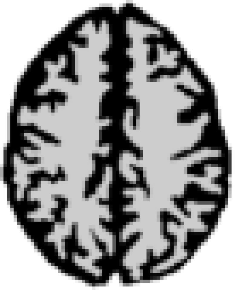
We simulated a clinical whole-body PET scanner operated in a 2D imaging mode. The scanner consists of 40 detector blocks arranged in a ring of diameter 90.9 cm. Each block contains 16 scintillation crystals. The individual crystal size is 4 mm (transaxial) ×12 mm (radial). An accurate system matrix was precomputed using a multi-ray tracing method that models the solid angle effect and photon penetration (Huesman et al., 2000). A Hoffman brain phantom shown in Figure 1 was forward projected to generate a noise-free sinogram. Noisy realizations were obtained by introducing independent Poisson noise to the noiseless projection. Two different count levels (250k and 500k) were examined. The mean of scattered and random events was assumed to be uniform across all sinogram bins. The final sinogram contains about 30% randoms and scatters. Images were reconstructed into a 102×102 pixel array of 2-mm square pixels using MAP-EM algorithm with a quadratic penalty function (De Pierro, 1995).

Figure 1.

The digital Hoffman brain phantom.

For quantitative evaluation, we compared the CVLL with the true log-likelihood function. We studied the mean and variance of the CVLL as a function of different cross-validation count levels (1%, 5%, 10%, 25%, 50% and 100%) of the reconstruction counts level, (which are equivalent to α = 100, 20, 10, 4, 2, 1, respectively). We computed the theoretically predicted variance using Equation (5) and validated the results using the sample variance from 500 independent realizations.

To examine the importance of datasets independence, we generate a series of cross-validation datasets by combining y₂ and y₁ with different ratio as

$${\mathit{y}}_m=(1-\xi ){\mathit{y}}_1+\xi {\mathit{y}}_2$$

with ξ = 0, 0.2, 0.3, 0.5, 1. Note ξ = 0 represents the true cross validation and ξ = 1 is completely self-validation, because datasets y₁ and y₂ are independent. The CVLL will be calculated using equation (3) with y₁ replaced by y_m. The reconstructed dataset y₂ remains the same.

3.2. Patient data study

The clinical data come from a Toshiba whole-body TOF PET/CT. The scanner consists of 40 detector blocks arranged in a ring of diameter 90.9 cm. Each block contains 16×48 lutetium-based scintillation crystals. The individual crystal size is 4 mm (transaxial) × 4 mm (axial) × 12 mm (radial). The timing resolution is approximately 400 ps. For a whole-body scan, eight 50% overlapping bed positions were combined into one dataset with 216 virtual rings in the axial direction. The dataset was divided into 4 independent identically distributed (i.i.d.) datasets with a total number of counts about 115 million each. One dataset was used for reconstruction and the other three datasets were used to generate cross-validation datasets by resampling the list-mode data. Resampling means to randomly choose a certain number of events from the other three datasets without replacement. Here “without replacement” means one event cannot appear twice in a single realization. One hundred realizations were generated at different count levels to compute the mean and standard deviation of the CVLL difference. An ordered-subset list-mode MAP-EM algorithm was used to reconstruct images, with 10 subsets and 5 iterations. Images were reconstructed using 150×150×216 voxels with a voxel size of 4×4×4 mm³. The attenuation factors were obtained from the CT scan. The normalization factors were computed based on a uniform cylinder scan. Randoms were estimated using the delayed window method. Scatters were estimated using the single-scatter simulation.

In addition to the quadratic penalty, we also studied a patch-based Fair penalty which has a form of

$$U(\mathit{x})=\sum _j\varphi \left(\sqrt{\sum _{k\in N_j}{\omega }_{\mathit{\text{jk}}}\sum _{l=1}^{n_l}{h}_l{(x_{j_l}-x_{k_l})}^2}\right)$$

where j_l denotes the lth voxel in the patch of voxel j, k_l denotes the lth voxel in the patch of voxel k. n_l is the total number of voxels in a patch. h_l is a positive weighting factor equal to the normalized inverse spatial distance between voxel j_l and voxel j with

$$\sum _{l=1}^{n_l}{h}_l=1$$

ϕ(t) is the Fair (a.k.a Lange) function

$${\varphi }_{\text{Fair}}(t)=\delta (\frac{|t|}{\delta }-\text{log}(1+\frac{|t|}{\delta }))$$

The derivative of the Fair function is

$${\varphi }_{\text{Fair}}^{\prime }(t)=\frac{t}{|t|+\delta }$$

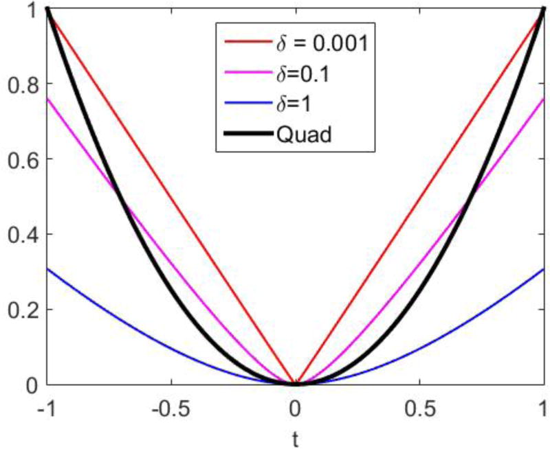
Therefore, the Fair function is equivalent to L₁ penalty when δ ≪ |t|, and approaches a quadratic function when δ ≫ |t|, as shown in Figure 2.

Figure 2.

Fair penalty functions with different δ.

4. Results

4.1. Simulation results

4.1.1 Mean and variance of CVLL

Figure 3 shows the reconstructed images using the quadratic penalty with different regularization strengths. The count level for the images in the top row is 250K and for the bottom row is 500K. As expected, the image becomes smoother from left to right as the regularization strength increases. The β values were chosen to show a range of reconstructed images that include both un-regularized images and over-smoothed images.

Figure 3.

Reconstructed images of Hoffman brain phantom. From left to right: β = 0, 2⁻¹⁷, 2⁻¹⁶, 2⁻¹⁵, 2⁻¹⁴, 2⁻¹³, 2⁻¹², 2⁻¹¹, 2⁻¹⁰. Top row: count level of 250K. Bottom row: count level of 500K.

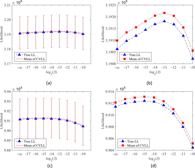
Figure 4 compares the true log-likelihood (LL) and CVLL at different count levels. The cross-validation count level is the same as the reconstruction count level (i.e., α = 1). The error bars were estimated from 500 independent realizations. We can see that as the regularization strength varies, there is a maximum point in the true log-likelihood curve. It is consistent with our knowledge that a proper regularization parameter can reduce the noise in reconstructed images and improve image quality, but a poorly selected regularization parameter, either too large or too small, will result in worse reconstructed images. More importantly, the CVLL curves yield the same maximum point as the true log-likelihood. Hence, the CVLL can be used to select regularization parameters that maximize the true log-likelihood without knowing the ground truth. Comparing Figure 4 (b) and (d), we can see that when the count level decreases, the optimum regularization parameters increase. This is as expected because noisier datasets require stronger regularization strength to suppress the noise. Finally, as predicted, the CVLL is an unbiased estimation of the true log-likelihood. Although the variance of the absolute CVLL value is much larger than the difference of the mean, it does not prevent us from choosing the optimal regularization parameters because the CVLL values of different β are highly correlated. In fact, all 500 CVLL curves yields the same optimal parameters as the true log-likelihood.

Figure 4.

Comparison of the true log-likelihood and CVLL as a function of regularization parameter β for the quadratic penalty. (a): count level of 250K. (b): (a) without error bar. (c) count level of 500K. (d): (c) without error bar.

4.1.2. Mean and variance of CVLL difference

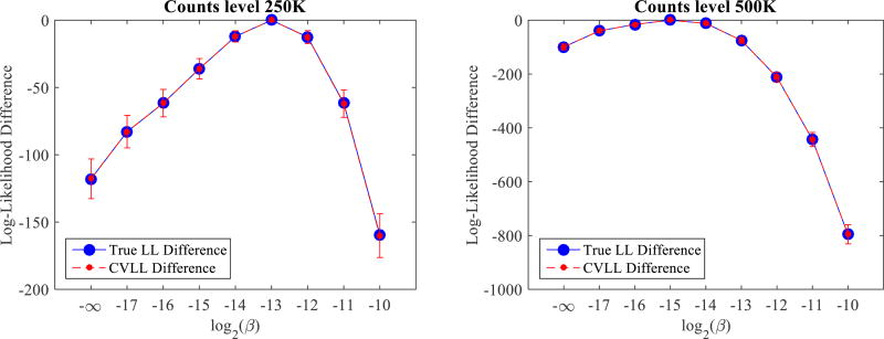
Figure 5 shows the mean and standard deviation of the CVLL difference with comparison to the true log-likelihood difference. All curves are normalized to their peak values. We can see that the CVLL difference predict the true LL difference very well and that the optimal β values (2⁻¹³ for 250K and 2⁻¹⁵ for 500K) are reliable with the current count level (α = 1) for cross validation. It also shows that as β moves away from the reference β_r, the standard deviation of CVLL difference increases. This is expected because the difference between x̂_β and x̂_βr increases.

Figure 5.

The mean and standard deviation of CVLL difference. Left: 250K. Right: 500K.

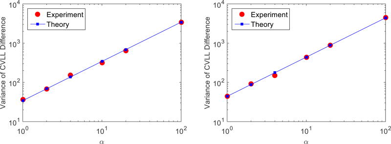
Figure 6 shows that the variance of the CVLL difference as a function of cross-validation count level. We replaced the noiseless data ȳ(x)_i in Equation (5) with noisy data y_1,i. Each experimental point in the figure was obtained by the average of 500 independent noisy realizations. The standard deviation of the variance estimation is smaller than the size of the symbol (not shown). The results show that the variance of CVLL difference is inversely proportional to the cross-validation count level, as predicted by Equation (5). Therefore, with an estimate of the variance at a given count level, one can easily predict the variance of the CVLL difference at any other count level, which is useful to find the minimum number of events for the cross validation to get a reliable estimate of an optimal β. For example, if the number of counts for cross validation is doubled, the variance of the CVLL difference is going to be halved. Hence, if the variance of CVLL is desired to be reduced by a factor of n, the number of events for cross validation should be increased by a factor of n.

Figure 6.

Variance of CVLL difference between β = 2⁻¹⁴ and β = 2⁻¹³ as a function of count ratio α. Left: reconstruction count level of 250K. Right: reconstruction count level of 500K.

As shown in Figure 5, the closest mean and standard deviation of CVLL difference are 12.0 ± 4.7 and 11.9 ± 4.9, for 250k and 500k count levels, respectively. Therefore, the maximum α that can be used while keeping the standard deviation less than the CVLL difference are ${(\frac{12}{4.7})}^2=6.5$ and ${(\frac{11.9}{4.9})}^2=5.9$ for 250k and 500k counts level, respectively, for this phantom image.

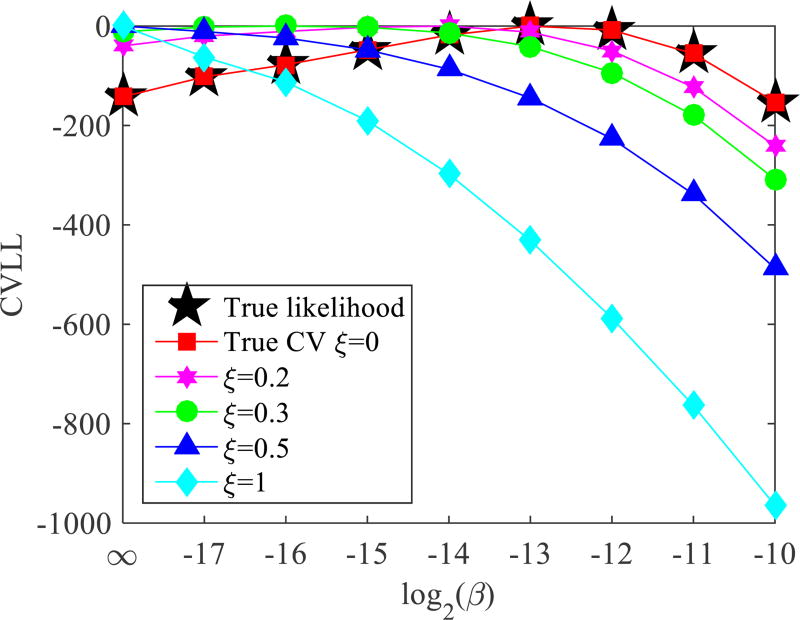
Figure 7 shows the importance of data independence in cross validation. The curve of black stars shows the true log-likelihood, and other color curves show the CVLL with validation data including different proportion (ξ) of reconstruction data. All curves are normalized with respect to their own peaks. As the correlation between the reconstruction data and validation data increases, the optimal β predicted by the CVLL becomes smaller and is pushed further away from the true optimal β. In the case of self-validation (ξ = 1), the predicted optimal β becomes zero and the reconstruction becomes the maximum likelihood estimation. These results clearly show that it is critical to maintain independence between the reconstruction data and validation data.

Figure 7.

Cross validation log likelihood when including different fraction of the reconstruction data. All curves are normalized with respect to their own peak values. The count level is 250k.

4.2. Patient data reconstructions

4.2.1. Parameter selection for the quadratic penalty

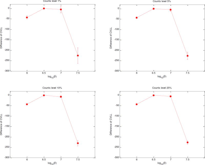
Figure 8 shows the mean and standard deviation of the CVLL difference computed from 100 realizations. The range of the β value is different from that used for the 2D simulation because the image intensity of the patient image is very different from that of the 2D phantom image. We studied the CVLL using 1%, 5%, 10%, or 25% count levels of the reconstruction dataset, which corresponds to α values of 100, 20, 10, 4, respectively. The reference point was chosen at β = 10^6.5 It yields the maximum CVLL across all cross-validation count levels, which is consistent with the analytical result that the estimation is unbiased, independent of the count level. With 1% cross-validation data, we can determine that β = 10^6.5 and β = 10⁷ result in higher CVLL values than either β = 10⁶ or β = 10^7.5. When the count level exceeds 10%, we are certain that β = 10^6.5 provides a higher CVLL than β = 10⁷. Therefore, β = 10^6.5 is the best regularization parameter among the regularization strengths examined here. However, since the CVLL values of β = 10^6.5 and β = 10⁷ are very close, the optimal β value is likely somewhere in-between, which can be estimated by fitting the three highest CVLL points to a quadratic function.

Figure 8.

Mean and standard deviation of the CVLL difference with respect to the reference point at β = 10^6.5 using different count levels in the cross validation.

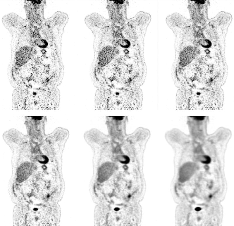
Figure 9 shows the reconstructed image of the patient data using different β values. The two best images selected by the CVLL are on the upper right (β = 3×10⁶) and lower left (β = 10⁷). Visually these images have acceptable image quality, i.e. neither too noisy nor too blurry.

Figure 9.

Reconstructed images with β = 0, 10⁶, 3×10⁶, 10⁷, 3×10⁷, 10⁸, using quadratic penalty function.

4.2.2. Parameter selection for the edge-preserving Fair penalty

The Fair penalty has two parameters, regularization strength β and a built-in tuning parameter δ. Hence we performed a two-dimension search for β and δ simultaneously. Since the mean intensity of reconstructed images is around 10⁻⁶ and the difference between neighboring voxels is on the same order, we chose δ = 2×10⁻¹², 2×10⁻⁷, 2×10⁻⁶, 2×10⁻⁵, which covers the transition range from the L₁ penalty to the quadratic penalty, according to the derivative of the Fair penalty.

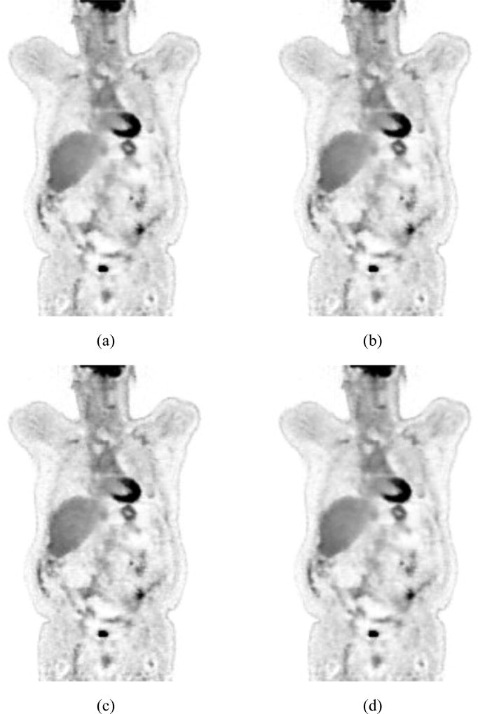
Table I shows the CVLL function value of the patch-based Fair penalty with different β and δ. The CVLL was calculated using α = 1, i.e. the count level for reconstruction and the count level for cross validation were the same. Since the CVLL curve has a single peak as a function of β, there is no need to calculate every slot in the table once we can identify the optimal β value. For small δ values, the optimal β value is 70, while for δ = 2×10⁻⁵, the optimal β value is 90. The latter matches the quadratic penalty result, because the Fair penalty approaches a quadratic penalty with parameter of $\frac{\beta }{\delta }=4.5\times {10}^6$. Figure 10 shows the reconstructed images of patch-based Fair penalty using the optimal β selected by the CVLL for different δ.

Table I.

CVLL of patch-based Fair penalty reconstruction.

β /δ	2×10−12	2×10−7	2×10−6	2×10−5
50	−22836997	−22837021	−22837104	−22837248
70	−22836963	−22836990	−22837078	−22837215
90	−22836975	−22837003	−22837086	−22837202
100	- -	- -	- -	−22837279

Figure 10.

Patch-based Fair penalty reconstruction. (a): δ = 2×10⁻¹², β = 70. (b): δ = 2×10⁻⁷, β = 70. (c): δ = 2×10⁻⁶, β = 70. (d): δ = 2×10⁻⁵, β = 90.

Table II shows the corresponding CVLL difference and its standard deviation. Since the variance is inversely proportional to the cross-validation count level, we can predict that the minimum fraction of events for a reliable estimate of the optimal β in the table. For example, when δ = 2×10⁻⁷, the CVLL difference between β = 70 and β = 90 is 13 with a standard deviation of 5.4. The maximum α value that we can use while still keeping the standard deviation to be less than 13 would be ${(\frac{13}{5.4})}^2=5.8$. Since the total counts for reconstruction is 115 million, the required number of events for cross validation is 115/5.8 = 19.8 million.

Table II.

CVLL difference and its standard deviation using β = 70 as the reference.

β / δ	2×10−12	2×10−7	2×10−6	2×10−5
50	−34 ± 6.6	−31 ± 6.5	−26 ± 5.9	−33 ± 4.2
70	0	0	0	0
90	−12 ± 5.5	−13 ± 5.4	−12 ± 4.9	13 ± 3.5
100	- -	- -	- -	−64 ± 5.1

5. Discussion

We have proposed a practical method to select regularization parameters in penalized likelihood reconstruction based on the cross-validation log-likelihood (CVLL). Statistical analysis shows that the CVLL function is an unbiased estimate of the log-likelihood calculated from the noise-free data. The proposed method does not require any prior knowledge of the true image nor the noiseless projection, and can be applied to a wide range of penalty functions and reconstruction algorithms. While a series of images with different regularization parameters need to be reconstructed to calculate the CVLL, there is no need to have multiple realizations. Therefore, the computational cost is greatly reduced compared with a lesion detectability study or Monte Carlo based SURE method. Simulation study shows that as the regularization strength varies, there is a maximum point in the true log-likelihood curve. More importantly, CVLL curve calculated from the proposed method reaches the maximum value at the same parameter as the true log-likelihood curve. In our simulation study, all 500 independent CVLL curves yield the same optimal parameter as the ground truth, and the mean of CVLL difference is unbiased, as predicted.

In practice, measured data need to be split into two parts, one for reconstruction and the other for cross validation. It is important to keep the reconstruction dataset and the cross validation dataset independent. Otherwise, the cross validation result will be problematic, as shown in Figure 7. Apparently, most events should be reserved for reconstruction and the number of events for cross validation should be kept as little as possible. The variance analysis provides a practical way to estimate the minimum number of cross-validation events to keep the CVLL result reliable. We can start with an initial α value (e.g., α = 6, which corresponds to 85% for reconstruction and 15% for cross-validation) and perform reconstruction and cross validation. Based on the resulting variance estimated using Equation (5) and the CVLL difference, we can then find the proper α value for a pre-determined variance as described in Section 4.2.2. The criterion that we used here is to have the standard deviation of the CVLL difference to be less than the CVLL difference itself, although a more (or less) stringent criterion could also be used. However, because a more stringent criterion would require more events in the validation dataset, a compromise has to be made to keep most events for reconstruction. Similarly the maximum α value is also affected by the step size of the regularization parameters. For the quadratic penalty in the simulation, we used a 2× ratio between adjacent β values, which corresponds to a 15–20% change in the FWHM of the spatial resolution measured using the method suggested by Gong et al (Gong et al., 2016). A larger ratio between β values would result in a larger CVLL difference and hence would require less validation events to satisfy the same criterion.

In the simulation, we have shown that the optimal regularization strength decreases, as the number of counts increases. It is consistent with our expectation that higher SNR data require less regularization. While the optimal regularization parameters can be affected by the number of counts, as well as the PET scanner characteristics, such as scanner geometry, detector resolution, field-of-view, etc., the applicability of the proposed method is not affected by these parameters because the CVLL is an unbiased estimate of the log-likelihood function computed using the noise free data regardless of the count level. We have shown that the proposed method can be applied to 2D non-TOF PET in the simulation as well as fully 3D TOF PET in the real experiment. In addition to the results shown in Section 4, we have also tested the simulation data with the count level ranging from 50k to 2M and found that the proposed method can identify the optimal β with similar accuracy and precision.

The results in Section 4 show that the perceptual quality of images selected by the proposed method is reasonable, although it may not be perfect, because the proposed method is based on an objective global figure of merit instead of human perception. It is possible that the proposed method does not agree with a subjective figure of merit, similar to the image mean squared error, which has been widely criticized, especially when dealing with perceptual important signals, such as speech and images (Wang and Bovik, 2009). Another interesting direction is to investigate the correlation between CVLL and local figure of merits, such as lesion contrast curve or lesion detectability.

6. Conclusion

We have presented a regularization parameter selection method based on the cross validation log-likelihood (CVLL) for penalized likelihood PET image reconstruction. The proposed method finds the optimal regularization parameter(s) that maximize the CVLL and does not require any knowledge of the true image. Our simulation and real data studies showed that the proposed method works well for PL reconstruction. Besides regularization parameter selection, the proposed method can also be applied to the selection of other reconstruction parameters, such as the iteration number and post-reconstruction filter in the ML-EM algorithm.

References

- Bardsley† JM, Laobeul ND. Tikhonov regularized Poisson likelihood estimation: theoretical justification and a computational method. Inverse Problems in Science and Engineering. 2008;16:199–215. [Google Scholar]
- Carlavan M, Blanc-FÉraud L. Sparse Poisson noisy image deblurring. IEEE Transactions on Image Processing. 2012;21:1834–1846. doi: 10.1109/TIP.2011.2175934. [DOI] [PubMed] [Google Scholar]
- De pierro AR. A modified expectation maximization algorithm for penalized likelihood estimation in emission tomography. IEEE Transactions on Medical Imaging. 1995;14:132–137. doi: 10.1109/42.370409. [DOI] [PubMed] [Google Scholar]
- Fessler JA, Rogers WL. Spatial resolution properties of penalized-likelihood image reconstruction: space-invariant tomographs. IEEE Transactions on Image processing. 1996;5:1346–1358. doi: 10.1109/83.535846. [DOI] [PubMed] [Google Scholar]
- Gong K, Cherry SR, Qi J. On the assessment of spatial resolution of PET systems with iterative image reconstruction. Phys Med Biol. 2016;61:N193–202. doi: 10.1088/0031-9155/61/5/N193. [DOI] [PMC free article] [PubMed] [Google Scholar]
- Hansen PC, O'leary DP. The use of the L-curve in the regularization of discrete ill-posed problems. SIAM Journal on Scientific Computing. 1993;14:1487–1503. [Google Scholar]
- Hudson HM, Larkin RS. Accelerated image reconstruction using ordered subsets of projection data. IEEE Transactions on Medical Imaging. 1994;13:601–609. doi: 10.1109/42.363108. [DOI] [PubMed] [Google Scholar]
- Hudson HM, Lee TC. Maximum likelihood restoration and choice of smoothing parameter in deconvolution of image data subject to Poisson noise. Computational Statistics & Data Analysis. 1998;26:393–410. [Google Scholar]
- Huesman RH, Klein GJ, Moses WW, Qi J, Reutter BW, Virador PR. List-mode maximum-likelihood reconstruction applied to positron emission mammography (PEM) with irregular sampling. IEEE Transactions on Medical Imaging. 2000;19:532–537. doi: 10.1109/42.870263. [DOI] [PubMed] [Google Scholar]
- Li Q, Asma E, Qi J, Bading JR, Leahy RM. Accurate estimation of the Fisher information matrix for the PET image reconstruction problem. IEEE transactions on medical imaging. 2004;23:1057–1064. doi: 10.1109/TMI.2004.833202. [DOI] [PubMed] [Google Scholar]
- Llacer J, Veklerov E, Coakley KJ, Hoffman EJ, Nunez J. Statistical analysis of maximum likelihood estimator images of human brain FDG PET studies. IEEE transactions on medical imaging. 1993;12:215–231. doi: 10.1109/42.232250. [DOI] [PubMed] [Google Scholar]
- Pawitan Y, O'sullivan F. Data-dependent bandwidth selection for emission computed tomography reconstruction. IEEE Transactions on Medical Imaging. 1993;12:167–172. doi: 10.1109/42.232245. [DOI] [PubMed] [Google Scholar]
- Qi J, Leahy RM. Resolution and noise properties of MAP reconstruction for fully 3-D PET. IEEE Transactions on Medical Imaging. 2000;19:493–506. doi: 10.1109/42.870259. [DOI] [PubMed] [Google Scholar]
- Qi J, Leahy RM. Iterative reconstruction techniques in emission computed tomography. Physics in Medicine and Biology. 2006;51:541–578. doi: 10.1088/0031-9155/51/15/R01. [DOI] [PubMed] [Google Scholar]
- Selivanov VV, Lapointe D, Bentourkia MH, Lecomte R. Cross-validation stopping rule for ML-EM reconstruction of dynamic PET series: effect on image quality and quantitative accuracy. IEEE Transactions on Nuclear Science. 2001;48:883–889. [Google Scholar]
- Stein CM. Estimation of the mean of a multivariate normal distribution. The Annals of Statistics. 1981:1135–1151. [Google Scholar]
- Thompson AM, Brown JC, Kay JW, Titterington DM. A study of methods of choosing the smoothing parameter in image restoration by regularization. IEEE Transactions on Pattern Analysis and Machine Intelligence. 1991;13:326–339. [Google Scholar]
- Wang Z, Bovik AC. Mean squared error: love it or leave it? A new look at signal fidelity measures. IEEE Signal Processing Magazine. 2009;26:98–117. [Google Scholar]
- Yang L, Zhou J, Ferrero A, Badawi RD, Qi J. Regularization design in penalized maximum-likelihood image reconstruction for lesion detection in 3D PET. Physics in Medicine and Biology. 2013;59:403–419. doi: 10.1088/0031-9155/59/2/403. [DOI] [PMC free article] [PubMed] [Google Scholar]
- Zanella R, Boccacci P, Zanni L, Bertero M. Efficient gradient projection methods for edge-preserving removal of Poisson noise. Inverse Problems. 2009;25:045010. [Google Scholar]
- Zhou J, Qi J. Monte Carlo SURE-based regularization parameter selection for penalized-likelihood image reconstruction; 2014 IEEE 11th International Symposium on Biomedical Imaging (ISBI); 2014. pp. 1095–1098. [Google Scholar]