Artifact removal in the context of group ICA: A comparison of single‐subject and group approaches

Abstract

Independent component analysis (ICA) has been widely applied to identify intrinsic brain networks from fMRI data. Group ICA computes group‐level components from all data and subsequently estimates individual‐level components to recapture intersubject variability. However, the best approach to handle artifacts, which may vary widely among subjects, is not yet clear. In this work, we study and compare two ICA approaches for artifacts removal. One approach, recommended in recent work by the Human Connectome Project, first performs ICA on individual subject data to remove artifacts, and then applies a group ICA on the cleaned data from all subjects. We refer to this approach as Individual ICA based artifacts Removal Plus Group ICA (IRPG). A second proposed approach, called Group Information Guided ICA (GIG‐ICA), performs ICA on group data, then removes the group‐level artifact components, and finally performs subject‐specific ICAs using the group‐level non‐artifact components as spatial references. We used simulations to evaluate the two approaches with respect to the effects of data quality, data quantity, variable number of sources among subjects, and spatially unique artifacts. Resting‐state test–retest datasets were also employed to investigate the reliability of functional networks. Results from simulations demonstrate GIG‐ICA has greater performance compared with IRPG, even in the case when single‐subject artifacts removal is perfect and when individual subjects have spatially unique artifacts. Experiments using test–retest data suggest that GIG‐ICA provides more reliable functional networks. Based on high estimation accuracy, ease of implementation, and high reliability of functional networks, we find GIG‐ICA to be a promising approach. Hum Brain Mapp 37:1005–1025, 2016. © 2015 Wiley Periodicals, Inc.

INTRODUCTION

Independent component analysis (ICA) has been widely applied to identify maximally independent sources from a set of observed data. As a data driven technique, ICA has some appealing advantages over conventional techniques for extracting brain functional networks from functional magnetic resonance imaging (fMRI) data. Different from the traditional general linear model (GLM) method, there is no requirement of deciding a hemodynamic response function or a specific time series while applying ICA. In addition, ICA does not require users to select prior regions of interest (ROI), whose selection could be difficult due to that the resulting networks are sensitive to their shape, location and intersubject variability [Du et al., 2012]. Therefore, ICA is applicable for complex task‐related experiments [Jarrahi et al., 2015; van de Ven et al., 2008] and resting‐state experiments with no explicit stimuli or task [Baggio et al., 2015; Du et al., 2015].

There are two ways to apply ICA on fMRI data analysis: spatial ICA [McKeown et al., 1998] and temporal ICA [Calhoun et al., 2001b]. Among the ICA‐based techniques, spatial ICA (sICA) is by far the most widely used approach, which decomposes the individual‐subject fMRI data matrix (size: number of time points $\times$ number of voxels) as a production of time courses (TCs) matrix (size: number of time points $\times$ number of components) and spatially independent components (ICs) matrix (size: number of components $\times$ number of voxels). The meaningful ICs are regarded as brain functional networks, and the voxels with high z‐scores in each functional network indicate the coherently activated regions. The corresponding TC of one functional network reflects the temporal fluctuation of the network. The remainder of this article is focused on sICA, so in the following ICA is used to denote sICA for simplicity.

Although ICA has been successful in the analysis of fMRI data, one of the challenges is in labeling ICs, which include not only meaningful functional networks, but also various artifacts‐related components arising from imaging and non‐neural physiological activity. In addition, the other shortcoming of ICA is that the number of sources is unknown. Although the number of sources can be estimated by information theoretic principles, such as a modified minimum description length (MDL) criteria [Li et al., 2007], different methods could result in desperate numbers [Zuo et al., 2010]. It is also known that the order of the ICs obtained from individual‐subject ICA is random, which makes the ICs of different subjects not directly comparable. Therefore, issues like identifying functional networks, deciding the number of sources, as well as matching the estimated ICs across subjects become more challenging when analyzing multi‐subject fMRI data.

In multi‐subject applications of ICA to fMRI data, typically one of two approaches is adopted [Calhoun et al., 2009]. The first approach applies ICA to each subject's data and establishes correspondence of ICs across subjects using subjective identification [Calhoun, 2001; McKeown et al., 1998], spatial matching with a predefined template [Greicius et al., 2004], clustering [Esposito et al., 2005; Moritz et al., 2003], or cross‐correlation [Schopf et al., 2010]. However, sometimes it is difficult to effectively establish correspondence of functional networks across subjects due to that some identified networks from different subjects are not similar enough to match. The problem could become more troublesome in the case where the estimated numbers of components from different subjects are various or disparate. An alternative approach, often referred to as group ICA [Beckmann et al., 2009; Calhoun and Adali, 2012; Calhoun et al., 2001a, 2009], implements a group‐level ICA on all data, and then computes subject‐specific ICs and their associated TCs based on the estimated group ICs. Group ICA establishes direct correspondence of ICs across subjects, avoiding the difficulties of matching components. Group ICA approaches include spatial concatenation [Svensen et al., 2002], temporal concatenation [Beckmann et al., 2009; Calhoun et al., 2001a, 2009] and tensor organization [Beckmann and Smith, 2005; Lee et al., 2008] methods, and the temporal concatenation methods are most widely applied. In order to reconstruct the individual‐subject results, typical temporal concatenation based group ICA approaches utilize either PCA‐based back‐reconstruction [Calhoun et al., 2001a; Erhardt et al., 2011] or regression‐based [Beckmann et al., 2009; Erhardt et al., 2011] method, both of which can capture moderate degrees of individual variability well [Allen et al., 2012], but may not be optimal for artifacts that can be completely unique across subjects.

In this article, we study and compare two approaches for artifacts removal in applying ICA to multi‐subject fMRI data. One approach, currently recommended in recent work from the Human Connectome Project [Smith et al., 2013], first performs ICA on individual‐subject data to remove artifacts, and then applies a dual regression based group ICA on the cleaned data of all subjects. We refer to this approach as Individual ICA based artifacts Removal Plus Group ICA (IRPG). IRPG is well‐suited for extreme intersubject variability in artifacts sources, but the difficulties of identifying artifacts‐related ICs for each individual data as well as determining the appropriate number of ICs to estimate may pose problems in practical application. This is particularly the case if many subjects are involved, although machine learning approaches (e.g., training classifiers) can help mitigate the difficulties of artifacts identification to a degree. There are several techniques to automatically identify artifacts‐related ICs, though most rely on some variant of supervised learning. Perlbarg et al. [2007] removed artifacts by matching ICs with known spatial patterns of physiological noise. De Martino et al. [2007] represented ICs in a multidimensional space of descriptive measures, “IC fingerprints,” which were then used to classify the ICs by feeding the features into a support vector machine. Tohka et al. [2008] proposed an improved decision tree method with a richer set of spatial and temporal features for artifacts removal. [Griffanti et al., 2014; Salimi‐Khorshidi et al., 2014] used a hierarchical fusion of classifiers to recognize artifacts associated ICs based on more than 180 features. Sochat et al. [2014] adopted a sparse logistic regression with elastic net regularization method based on more features to automatically identify artifacts, and showed a high accuracy of classification. In this work, we apply a toolbox released by Sochat et al. [2014] to identify subject‐level artifact ICs in IRPG.

An alternative approach, called Group Information Guided ICA (GIG‐ICA) [Du and Fan, 2013], extracts group ICs by implementing group‐level ICA on all data, and then uses the estimated non‐artifact group ICs as references to compute individual functional networks based on a new one‐unit ICA with reference algorithm [Du and Fan, 2011; Du and Fan, 2013]. Compared with IRPG, GIG‐ICA does not require identification of artifacts for each subject. Instead, GIG‐ICA takes advantage of the fact that components which show similarity among subjects (e.g., the networks of interest) tend to not be corrupted by the unique artifacts [Calhoun et al., 2001a]. GIG‐ICA allows for additional flexibility in individual subjects by re‐optimizing the independence of subject‐specific functional networks, while still preserving the correspondence of functional networks across subjects. GIG‐ICA estimates the individual functional networks using a multiple‐objective optimization framework, which simultaneously optimizes the independence of individual networks as well as the correspondence between group ICs and individual networks. A previous study [Du and Fan, 2013] indicated that GIG‐ICA is able to achieve functional networks with higher accuracy compared with traditional group ICA methods, which include the PCA‐based back‐reconstruction algorithms (i.e., GICA1, GICA2, and GICA3) [Calhoun et al., 2001a; Erhardt et al., 2011] as well as the dual regression based approach. In addition, GIG‐ICA has been shown to be successful in identifying the subtle difference among symptom‐related diseases, such as schizophrenia, bipolar disorder, and schizoaffective disorder [Du et al., 2014b, 2015].

In the following sections, we firstly describe IRPG and GIG‐ICA methods in detail, and then evaluate and compare their performances using both simulations and real fMRI data. In addition, we also examine the traditional group ICA (GICA) approach without removing artifacts for a comparison. Simulations‐based experiments assess the accuracy of ICs/TCs obtained from the three methods using datasets with different quality and quantity, variable number of sources among subjects, and unique artifacts. We also perform those methods on resting‐state test‐retest fMRI data to extract functional networks. Since the ground truth for real data is unknown, reliability measures are used to evaluate the estimated functional networks, consistent with previous studies [Griffanti et al., 2014; Zuo et al., 2010]. We predict that GIG‐ICA would more accurately and reliably estimate individual functional networks, since the method optimizes the independence of subject‐specific networks. Preliminary results of this study have been reported in a article [Du et al., 2014a].

MATERIALS AND METHODS

In this section, we introduce the frameworks and relevant parameters for IRPG, GIG‐ICA and GICA, and then describe simulations and real fMRI data based experiments.

Algorithmic Frameworks

IRPG

The framework of IRPG is shown in Figure 1A. It involves the following steps:

Figure 1.

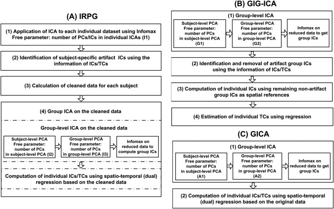
Frameworks of methods. (A) Framework of Individual ICA based artifacts Removal Plus Group ICA (IRPG). IRPG involves individual ICA, identification of subject‐specific artifact ICs, calculation of cleaned data for each subject, group‐level ICA on the cleaned data, and computation of individual ICs/TCs using dual regression. (B) Framework of Group Information Guided ICA (GIG‐ICA). GIG‐ICA involves group‐level ICA on group data, identification and removal of artifact group ICs, computation of individual ICs using the remaining non‐artifact group ICs as spatial references, and estimation of individual TCs using regression. (C) Framework of traditional Group ICA (GICA). GICA involves group‐level ICA on group data and computation of individual ICs/TCs using dual regression.

1. Application of ICA with Infomax algorithm [Bell and Sejnowski, 1995] on each individual‐subject dataset.

2. Identification of subject‐specific artifact ICs.

3. Calculation of cleaned data for each subject.

4. Group ICA on the cleaned data from all subjects.

In the step (2), for simulations, the artifact ICs are identified based on the information of ground‐truth artifact ICs; for real fMRI data, the artifact ICs are selected using a machine learning approach. In the step (3), for real fMRI data, we regress the artifact ICs related TCs out of the original data to obtain the cleaned individual data, which is consistent with the articles from the Human Connectome Project [Griffanti et al., 2014; Salimi‐Khorshidi et al., 2014]. The used equation is: $X_{\mathrm{n}\mathrm{e}\mathrm{w}}=X_{\mathrm{o}\mathrm{l}\mathrm{d}}‐{\mathrm{T}\mathrm{C}}_{\mathrm{A}\mathrm{r}\mathrm{t}}·({{\mathrm{T}\mathrm{C}}_{\mathrm{A}\mathrm{r}\mathrm{t}}}^{+}·X_{\mathrm{o}\mathrm{l}\mathrm{d}})$, where ${\mathrm{T}\mathrm{C}}_{\mathrm{A}\mathrm{r}\mathrm{t}}$ denotes the artifact ICs related TCs, $X_{\mathrm{o}\mathrm{l}\mathrm{d}}$ denotes the original data matrix, $X_{\mathrm{n}\mathrm{e}\mathrm{w}}$ denotes the cleaned data, and $+$ denotes the pseudo‐inverse. Since simulations are generated based on ICA model, we reconstruct the new individual data based on the non‐artifact ICs using equation: $X_{\mathrm{n}\mathrm{e}\mathrm{w}}={\mathrm{T}\mathrm{C}}_{\mathrm{N}\mathrm{o}\mathrm{n}\mathrm{A}\mathrm{r}\mathrm{t}}·{\mathrm{I}\mathrm{C}}_{\mathrm{N}\mathrm{o}\mathrm{n}\mathrm{A}\mathrm{r}\mathrm{t}}$, where ${\mathrm{I}\mathrm{C}}_{\mathrm{N}\mathrm{o}\mathrm{n}\mathrm{A}\mathrm{r}\mathrm{t}}$ and ${\mathrm{T}\mathrm{C}}_{\mathrm{N}\mathrm{o}\mathrm{n}\mathrm{A}\mathrm{r}\mathrm{t}}$ denote the non‐artifact ICs and the corresponding TCs, respectively. For simulations, we also investigate the performance of IRPG with regression based artifacts removal, and report the relevant results in Supporting Information. In the step (4), subject‐level PCA on each subject's dataset and a second group‐level PCA on the reduced data [Calhoun et al., 2001a] are implemented first for dimension reduction. And then, a group‐level ICA using Infomax algorithm is performed on the reduced group data to compute group ICs. Finally, subject‐specific ICs/TCs are calculated using a spatio‐temporal (dual) regression method [Beckmann et al., 2009; Calhoun et al., 2004; Erhardt et al., 2011; Filippini et al., 2009], which was also employed in Human Connectome Project articles [Griffanti et al., 2014; Salimi‐Khorshidi et al., 2014]. The equations are: $\mathrm{T}\mathrm{C}\mathrm{s}=X_{\mathrm{n}\mathrm{e}\mathrm{w}}·{\mathrm{G}\mathrm{I}\mathrm{C}\mathrm{s}}^{+}$, $\mathrm{I}\mathrm{C}\mathrm{s}={\mathrm{T}\mathrm{C}\mathrm{s}}^{+}{·X}_{\mathrm{n}\mathrm{e}\mathrm{w}}$, where $\mathrm{G}\mathrm{I}\mathrm{C}\mathrm{s}$, $\mathrm{I}\mathrm{C}\mathrm{s}$, and $\mathrm{T}\mathrm{C}\mathrm{s}$ denote the group ICs, individual ICs, and individual TCs, respectively. Individual ICs are then z‐scored to facilitate further statistical analysis.

Some important free parameters in the IRPG framework as displayed in Figure 1A include the number of PCs/ICs used in the individual ICAs, denoted as $\mathrm{I}1$, the number of PCs used in the subject‐level PCAs, denoted as $\mathrm{I}2$, and the number of PCs/ICs used in the group‐level PCA/ICA, denoted as $\mathrm{I}3$. It is worth noting that $\mathrm{I}2$ should be bigger than or equal to $\mathrm{I}3$ to minimize loss of information from individual data [Erhardt et al., 2011].

GIG‐ICA

The framework of GIG‐ICA shown in Figure 1B involves the following steps:

1. Application of group‐level ICA to all subjects’ datasets.

2. Identification and removal of artifact group ICs.

3. Computation of individual ICs via a multiple‐objective optimization framework using non‐artifact group ICs as spatial references [Du and Fan, 2011, 2013].

4. Estimation of individual TCs using regression: $\mathrm{T}\mathrm{C}\mathrm{s}=\mathrm{X}·{\mathrm{I}\mathrm{C}\mathrm{s}}^{+}$, where $\mathrm{X}$ is the individual‐subject data, and $\mathrm{I}\mathrm{C}\mathrm{s}$ denotes the estimated individual ICs matrix.

In the step (1), subject‐level PCA on individual dataset and group‐level PCA on the reduced data are implemented, and then a group‐level ICA with Infomax is performed on the reduced data to compute group ICs. In the step (2), for simulations, artifact group ICs are identified based on the information of ground‐truth artifact ICs; for real fMRI data, artifact group ICs are selected manually according to features of ICs and TCs. In the step (3), the multiple‐objective function optimization simultaneously optimizes the independence of individual ICs as well as the correspondence between individual ICs and group ICs. The independence of each individual IC is estimated by its negentropy, denoted by $J={\left\{E\left[G\left(S_I\right)\right]‐E\left[G\left(v\right)\right]\right\}}^2$, where $S_I$ is one subject‐specific IC to estimate, $v$ is a Gaussian variable with zero mean and unit variance, $G(·)$ is a nonquadratic function. The correspondence between individual IC and group IC is estimated by $F=E[S_I·S_G]$, where $S_G$ denotes one group IC that is z‐scored to zero mean and unit variance. The multiple‐objective function optimization problem is solved using a linear weighted sum technique, and a parameter $a$ [Du and Fan, 2011, 2013] as a weight to balance the two objectives is specified as 0.5. GIG‐ICA automatically generates z‐scored ICs.

Therefore, relevant free parameters in the GIG‐ICA include the number of PCs denoted as $\mathrm{G}1$ used in the subject‐level PCAs and the number of PCs/ICs denoted as $\mathrm{G}2$ used in the group‐level PCA/ICA. Similar to IRPG, $\mathrm{G}1$ should be bigger than or equal to $\mathrm{G}2$ for minimizing loss of information. For clarity, we use $\mathrm{G}3$ to denote the remaining number of group ICs after artifacts removal, although $\mathrm{G}3$ is not a parameter that needs to be chosen independently. Note that with the new one‐unit ICA with reference algorithm used at the single‐subject ICA stage, computation of non‐artifact individual ICs is not affected by the presence of artifact group ICs, thus accurate identification and removal of artifacts are less critical than that in the IRPG framework.

GIGA

The framework of GICA is shown in Figure 1C. The processing is similar to the step (4) of IRPG, except that GICA is performed on the original data and estimates all individual ICs including artifacts. Individual ICs from GICA are z‐scored for further analysis. Free parameters in the GICA framework include the number of PCs denoted as $\mathrm{A}1$ used in the subject‐level PCAs and the number of PCs/ICs denoted as $\mathrm{A}2$ used in the group‐level PCA/ICA. For GICA, $\mathrm{A}1$ and $\mathrm{A}2$ are set to the same values of $\mathrm{G}1$ and $\mathrm{G}2$, respectively, considering that both GIG‐ICA and GICA implement group‐level ICA on the original data rather than the cleaned data.

In this article, the dual regression based GICA method is applied to simplify comparisons with IRPG, since Human Connectome Project articles [Griffanti et al., 2014; Salimi‐Khorshidi et al., 2014] used dual regression based method. However, PCA‐based GICA methods [Erhardt et al., 2011], which have been shown to have a comparable performance with dual regression in terms of the estimation of individual ICs/TCs, also deserve to be examined in future work.

Experiments Using Simulations

Multi‐subject fMRI‐like data were generated using the SimTB toolbox [Allen et al., 2012; Erhardt et al., 2012]. For each of $M$ subjects, simulated dataset was generated under a linear mixture model using $C$ fMRI‐like source images ( $148\times 148$ pixels) and associated time courses (150 or less time points in length, see Table 1). Rician noise was added to the linear mixture of sources with a specified contrast‐to‐noise ratio (CNR). Repetition time (TR) was 2 s/sample. $M$ was the number of simulated subjects, and $C$ denoted the number of simulated sources for each subject. In the following experiments, $M=10$, $C=8 \mathrm{o}\mathrm{r} 7$. The ratio of the number of pixels in mask to the number of sources was greater than 2,000, which was consistent with the real case of nearly 60,000 voxels in brain mask and 20 to 30 components to be estimated [Abou‐Elseoud et al., 2010]. Among $C$ sources, some were labeled as non‐artifact sources, while others were labeled as artifacts. To simplify the description, we denoted the $j^{\mathrm{t}\mathrm{h}}$ source of the $i^{\mathrm{t}\mathrm{h}}$ subject as $S_{i,j} (i=1,\cdots ,M; j=1,\cdots ,C)$. In our work, $S_{i,j}$ was considered as a non‐artifact source when $j=1,\cdots ,K$, and was considered as an artifact source when $j=K+1,\cdots ,C$. $K$ was the number of the simulated non‐artifact sources. Parameters of simulations and three methods in the following experiments for assessing the effect of data quality (CNR), data quantity (number of time points), variable number of sources, and spatially unique artifacts are summarized in Table 1.

Table 1.

Parameters of simulations and methods used in simulations‐based experiments

Parameters	Experiment 1 (data quality)	Experiment 1 (data quantity)	Experiment 2 (variable number of sources)		Experiment 3 (spatially unique artifacts)
$C$	8	8	8 ( $i=1,\cdots ,5)$; 7 ( $i=6,\cdots ,10)$	8
$K$	7	7	6	7
CNR	0.5–2	1	2	2
No. time points	150	40–120	150	150
$\mathrm{I}1$	8	8	$C$, 7, and 8 in separate tests	8
$\mathrm{I}2$	7	7	6	7
$\mathrm{I}3$	7	7	6	7
$\mathrm{G}1$	8	8	8	8
$\mathrm{G}2$	8	8	7 and 8 in separate tests	8
$\mathrm{G}3$	7	7	6	7
$\mathrm{A}1$	8	8	8	8
$\mathrm{A}2$	8	8	7 and 8 in separate tests	8

Experiment 1: Effect of data quality and quantity

To evaluate the effect of data quality (i.e., CNR), 16 datasets with different CNRs ranging from 0.5 to 2 with intervals of 0.1 were generated. The simulated number of time points was 150 for the 16 datasets. We similarly explored a loss in data quantity by keeping the CNR in each data fixed at 1, but varying the number of time points from 40 to 120 in steps of 20. Figure 2 shows the sources and their associated time courses for the simulated data of two subjects, as well as the spatial variability of sources across subjects. For different subjects, each of the eight sources was generated through adding subject‐specific variability to a common map, so sources were more or less spatially consistent across subjects. Spatial variability was generated by assigning random translations (mean of 0 and standard deviation (SD) = 6 pixels), rotations (mean of 0, SD = 4 degrees, and spreads (mean = 2, SD = 0.03)) to subject sources. Subject‐specific variability also included temporal variation of TCs. In this simulation, the eighth source with high frequency TC was chosen as the artifact source.

Figure 2.

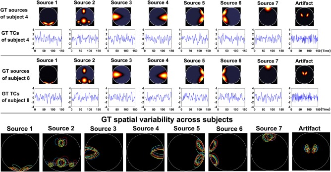
Ground‐truth (GT) sources and their associated TCs for the simulated data of two subjects in Experiment 1. The bottom row shows the spatial variability of sources across subjects in Experiment 1 (spatial variability was similar in other Experiments); each color denotes the source contours of a different subject. [Color figure can be viewed in the online issue, which is available at http://wileyonlinelibrary.com.]

To simply show the independence among the simulated sources of each subject, we computed the absolute values of Pearson correlation coefficients between all pairs of sources as well as the normalized mutual information [Du and Fan, 2013] between all pairs of sources, and then averaged the absolute correlation or the normalized mutual information values to obtain summarized measures for this subject. The smaller values of these measures represent higher independence or lower dependence. Similarly, the independence measures among the simulated time courses were calculated. Figure S1 in Supporting Information shows the independence measures for data with different CNRs and data with different numbers of time points. While it is not easy to generate sources/time courses with complete independence, it is seen that the simulated sources/time courses had relatively low dependence with each other. Since it is acknowledged that some brain functional networks can have spatial overlap to some extent, we think the datasets are acceptable.

As displayed in Table 1, for IRPG, $\mathrm{I}1$ was specified as the real number of sources, $C$ (i.e., 8). Both $\mathrm{I}2$ and $\mathrm{I}3$ were set to $C‐1$ reflecting the true number of remaining components with perfect artifacts removal, since in this experiment a single artifact IC was always identified by finding the individual IC with the largest absolute value of Pearson correlations to the respective artifact template. The artifact template for the $i^{\mathrm{t}\mathrm{h}}$ subject in IRPG was defined as the subject‐specific ground‐truth (GT) artifact source $S_{i,8}$. For GIG‐ICA, both $\mathrm{G}1$ and $\mathrm{G}2$ were set to $C$. For artifacts removal of GIG‐ICA, the group‐level artifact was accurately identified by finding the group IC with the largest absolute value of Pearson correlations to a artifact template $T_8$, which was generated by averaging the GT artifact sources across subjects. We defined

$$T_j=\frac{1}{N}{\sum }_{i=1}^N{S}_{i,j,}$$ (1)

where $N$ was the number of subjects that had source $S_{i,j}$. For GICA, similarly to GIG‐ICA, both $\mathrm{A}1$ and $\mathrm{A}2$ were set to $C$. Without removing artifacts, GICA estimated all $C$ ICs for each subject. For an equivalent comparison, we only used the matched non‐artifact individual ICs for the following evaluation.

To evaluate the spatial/temporal accuracy of each estimated subject‐specific non‐artifact IC/TC, we computed the absolute value of Pearson correlation coefficient between each IC/TC and the corresponding GT source/TC. The GT sources/TCs that correspond to the estimated subject‐specific ICs/TCs were identified by matching non‐artifact templates and the group ICs using a greedy algorithm. Using Eq. (1), the non‐artifact templates were computed as the averaged non‐artifact GT sources across subjects, i.e., $T_j (j=1,\cdots ,K$). Therefore, we obtained the spatial/temporal accuracy of each estimated subject‐specific IC/TC. After that, for each of those datasets with different CNRs or different numbers of time points, a two‐tailed paired t‐test was performed to compare the ICs (or TCs) accuracy of all subjects from GIG‐ICA with that from IRPG. Similarly, the ICs (or TCs) accuracy of all subjects from IRPG and that from GICA were also compared using a two‐tailed paired t‐test. The significance level was adjusted for P < 0.05. As a summary measure, we also calculated the mean of all ICs (or TCs) accuracy to reflect the overall IC (or TC) accuracy of one subject. In the following simulations‐based experiments, we used a similar procedure to evaluate the quality of ICs/TCs estimation.

Experiment 2: Effect of variable number of sources among subjects

Traditional group ICA methods often assume that all subject datasets have same number of components. However, the number of sources can vary across subjects, particularly the number of detectable artifacts. We evaluated the effect of subject datasets with different numbers of sources. Five subject datasets were simulated with eight sources, two of which were labeled as artifacts, while the other five subject datasets were simulated with seven sources, one of which was labeled as an artifact. Simulated data for such two subjects is shown in Figure 3. Figure S2A,B in Supporting Information show the independence measures of all subjects for the dataset.

Figure 3.

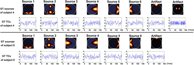
GT sources and their associated TCs of two subjects in Experiment 2. The above dataset has eight sources, of which the seventh and eighth are regarded as artifacts. The below dataset has seven sources, of which the seventh is regarded as an artifact. [Color figure can be viewed in the online issue, which is available at http://wileyonlinelibrary.com.]

Due to the varied number of individual sources, the parameters in those methods can have multiple choices, especially $\mathrm{I}1$ in IRPG, $\mathrm{G}2$ in GIG‐ICA and $\mathrm{A}2$ in GICA. For IRPG, we specified $\mathrm{I}1$ as $C$ (the subject's true number of sources), 7, or 8 in separate tests. When $\mathrm{I}1$ was set to $C$, the first five subjects data were decomposed to 8 ICs and the last five subjects were decomposed to 7 ICs at the individual ICA step. When $\mathrm{I}1$ was set to 7 or 8, all subjects data were decomposed to 7 or 8 ICs at the individual ICA step. Both $\mathrm{I}2$ and $\mathrm{I}3$ were specified as 6 due to that there were 6 non‐artifact sources in the simulated data. For GIG‐ICA, $\mathrm{G}1$ was set to 8, while $\mathrm{G}2$ was specified as 7 or 8 in separate tests. For traditional GICA, $\mathrm{A}1$ was set to 8, and $\mathrm{A}2$ was set to 7 or 8 in separate tests. Note that it is not possible to set the number of group ICs of GIG‐ICA or GICA as $C$, since group‐level ICA requires a single model order for all subjects.

When identifying the artifact ICs for IRPG and GIG‐ICA, absolute values of Pearson correlation coefficients were computed between the obtained ICs (individual ICs from IRPG or group ICs from GIG‐ICA) and the related artifact templates. The artifact templates used for IRPG were the subject‐specific GT artifact sources, thus the first five subjects had two artifact templates and the last five subjects had one artifact template. For GIG‐ICA, two artifact templates were calculated as $T_7$ and $T_8$ using the Eq. (1). ICs with absolute values of Pearson correlation coefficients exceeding a given threshold were considered as artifacts. The threshold was set to 0.7, which was empirically determined to accurately identify the artifacts for IRPG when $\mathrm{I}1$ was set to $C$. For GICA, only the six non‐artifact ICs were selected for comparison to the other methods.

Experiment 3: Effect of spatially unique artifacts

In the above experiments, artifact sources of different subjects were simulated by adding subject‐specific spatial variation to a common map. We know that group ICA approaches were proposed with the hypothesis that different subject datasets have common or similar spatial sources. However, in real data it is likely that spatially unique sources exist among subjects, particularly for artifacts. To investigate the performance of these approaches under this condition, greatly different artifact sources were generated for subjects. To be consistent with some types of artifacts observed in fMRI data [Kundu et al., 2012], these sources were simulated to have high‐frequency TCs. Figure 4 shows the simulated artifact sources and the related TCs of all 10 subjects. Figure S2C,D in Supporting Information show independence measures of all subjects for this dataset.

Figure 4.

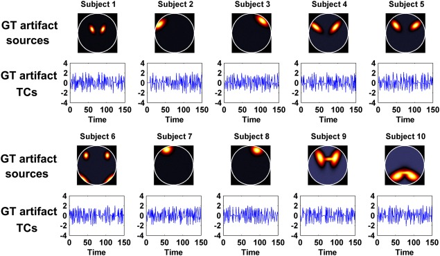
Simulated GT artifact source (the eighth source) and related TC for each subject in Experiment 3. [Color figure can be viewed in the online issue, which is available at http://wileyonlinelibrary.com.]

For IRPG, $\mathrm{I}1$ was specified as the real number of sources, $C$ (i.e., 8). In addition, $\mathrm{I}2$ and $\mathrm{I}3$ were specified as $C‐1$, since artifact of each subject was correctly identified in IRPG by finding the TC with the most high frequency power. In this experiment, we did not use spatial templates to identify the artifacts, as different subjects had very different artifact sources. In contrast, spectral information of TCs, which also can provide important information for artifacts removal in real application, was used to identify the artifacts. For GIG‐ICA, both $\mathrm{G}1$ and $\mathrm{G}2$ were specified as $C$. To identify the artifact group IC, we also used the spectral information of individual TCs. Based on all group ICs, preliminary individual TCs were computed using regression (in a manner identical to the GICA framework), then the artifact group IC was accurately identified as a component that generated high‐frequency individual TC. For GICA, both $\mathrm{A}1$ and $\mathrm{A}2$ were set to $C$, and only the non‐artifact individual ICs were used for comparative evaluation.

Experiments Using Resting‐State fMRI Data

Seventy five resting‐state fMRI datasets [Zuo et al., 2010] comprising 25 healthy participants (11 males; mean age 20.5 ± 8.4) with three scans were adopted in the experiment. Those datasets were downloaded from the website (https://www.nitrc.org/projects/nyu_trt/). Each dataset consisted of 197 contiguous EPI functional volumes (TR = 2,000 ms; TE = 25 ms; flip angle = 90°, 39 slices, matrix = 64 × 64; FOV = 192 mm; acquisition voxel size = 3 × 3 × 3 mm). Data of scan 2 and 3 were collected with interval of 45 min, 5 to 16 months (mean 11 ± 4) after scan 1. The participants were removed from the scanner between the scan 2 and the scan 3. The fMRI images were preprocessed using SPM8 (http://www.fil.ion.ucl.ac.uk/spm). The first 10 images were discarded, and the remaining 187 images were slice‐time corrected and realigned to the first volume for head‐motion correction. Subsequently, the images were spatially normalized to the Montreal Neurological Institute (MNI) EPI template and spatially smoothed with a 6 mm FWHM Gaussian kernel.

Each of the three methods including IRPG, GIG‐ICA, and GICA was applied to the 75 preprocessed datasets from three scans, resulting in individual networks with direct correspondence across those 75 datasets. Specifically, group‐level ICA involved in the step (4) of IRPG, the step (1) of GIG‐ICA, as well as the step (1) of GICA was performed on the 75 datasets rather than the separate 25 datasets from each scan. At the group‐level ICA step for those methods, ICASSO [Himberg et al., 2004] was used with 20 iterations to find reliable group ICs. To set the parameters for the three methods, we estimated the number of components for each of 75 datasets based on MDL, Akaike Information Criterion (AIC), and Kullback–Leibler Information Criterion (KIC) rules, respectively. As seen in Supporting Information Figure S3, the estimated dimensionality obtained from different rules varied. The maximum and mean dimensionality estimates across all criteria were 45 and 20, respectively. We set $\mathrm{I}1$ to the maximum, i.e., 45, since it preserves greater than 99% variance for all 75 datasets. $\mathrm{I}2$ was specified to the minimum value of remaining dimensions across subjects after artifacts removal. $\mathrm{I}3$ was tested using different values including 10 and 15, with the condition that $\mathrm{I}3<\mathrm{I}2$. For GIG‐ICA, $\mathrm{G}1$ was set to 45, and $\mathrm{G}2$ was set as a number larger than $\mathrm{I}3$ (based on the percentage of the number of identified individual‐subject artifacts in IRPG), due to that GIG‐ICA removes artifacts after group‐level ICA. As described in the following Results section, the percentage of the number of identified artifact ICs in IRPG was close to 50%, so we set $\mathrm{G}2$ to 20 and 30 for facilitating the comparisons between GIG‐ICA and IRPG. For GICA, $\mathrm{A}1$ and $\mathrm{A}2$ were set to the same values with $\mathrm{G}1$ and $\mathrm{G}2$, respectively.

To automatically identify individual‐subject artifact ICs in IRPG, we adopted a sparse logistic regression with elastic net regularization method as recently proposed by Sochat et al. [2014]. First, five raters independently labeled individual ICs from scan 1 (45 ICs × 25 datasets = 1,125 components) as “good” for networks, “bad” for artifacts, or “unknown” for components that could not be unambiguously identified as good or bad. ICs were evaluated based on visual inspection of the spatial maps, TCs, and spectra. Similar to a recent work [Salimi‐Khorshidi et al., 2014], those “unknown” components were treated as “good” components during classifier training to avoid removing valid neuronal signal. Based on the five sets of labels, the final label for each IC was determined by a simple majority. For automatic identification of artifacts, 249 features were computed form each IC and its related TC. These features along with the assigned labels were then used to train classifier and select features. The optimal parameters alpha and lambda in the model [Salimi‐Khorshidi et al., 2014] were first determined by grid search via maximization of 10‐fold cross validation accuracy, and then the classifier and features were obtained through training all 1,125 ICs. The output of the classifier is a set of weights corresponding to the contribution of each feature, and the non‐zero weights were used as input to the logistic regression to classify novel components. Using the model, individual‐subject ICs from scan 2 and scan 3 were automatically classified as “good” components and artifacts. For GIG‐ICA, we identified the artifact group ICs manually since expert identification is considered as the “gold standard”. Each group IC was checked with respect to the spatial map of IC, mean of individual TCs, and spectra of mean of individual TCs. Similar to the above Experiment 3 using simulations, preliminary individual TCs were computed using regression based on all group ICs. Subsequently, individual ICA with non‐artifact group ICs as references was applied to estimate the subject‐specific ICs in GIG‐ICA. Since traditional GICA estimated all ICs for each subject, the method did not require additional identification of the artifacts‐related ICs.

In order to compare the functional networks obtained from IRPG, GIG‐ICA, and GICA, we matched the functional networks from the three methods in condition of comparable parameters. Specifically, we matched the results under setting of $\mathrm{I}3$  = 10, $\mathrm{G}2$ = 20, $\mathrm{A}2$ = 20 and setting of $\mathrm{I}3$ = 15, $\mathrm{G}2$ = 30, $\mathrm{A}2$ = 30, respectively. Firstly, we matched the results from IRPG and GIG‐ICA based on the correlations between group ICs from the two methods using a greedy matching rule. Components with correlations larger than 0.5 were considered as the matched ICs. Secondly, we averaged the corresponding group ICs obtained from IRPG and GIG‐ICA to obtain the mean group ICs of the two methods. Finally, based on the mean group ICs of IRPG and GIG‐ICA as well as the group ICs from traditional GICA, we performed the other greedy matching procedure to match the ICs from IRPG and GIG‐ICA with the ICs from GICA. Thus, the corresponding functional networks from the three methods were identified. Note that the following evaluations were performed only for those matched functional networks. The parameters used in those methods and the numbers of the matched functional networks can be found in Table 2.

Table 2.

Parameters of methods for real fMRI data based experiments and the numbers of matched functional networks under different model order

Parameters	$\mathrm{I}1$	$\mathrm{I}2$	$\mathrm{I}3$	$\mathrm{G}1$	$\mathrm{G}2$	$\mathrm{G}3$	$\mathrm{A}1$	$\mathrm{A}2$	H
Value	45	16	10, 15	45	20, 30	12, 16	45	20, 30	10, 14

H: the number of matched functional networks across different methods.

Due to that the ground truth in real data is unknown, it is always difficult to determine optimal measures for evaluating methods. Quite often, the reliability of functional networks obtained from resting‐state test‐retest data of healthy subjects is used as an alternative [Griffanti et al., 2014; Guo et al., 2012; Zuo et al., 2010], assuming that corresponding functional networks in such data should be very similar. Zuo et al. [2010] computed intra class coefficients (ICCs) in networks between different scans as well as correlations between individual ICs and group ICs. Motivated by previous work [Smith et al., 2005], Griffanti et al. [2014] calculated the similarity of corresponding networks between all pairs of subjects.

Similarly, we evaluated the reliability of functional networks for IRPG, GIG‐ICA, and GICA, respectively. Firstly, for each network, voxel‐wise one‐sample t‐tests with false discovery rate (FDR) correction (P < 0.01) were performed across all 75 datasets to show the network patterns. And then, we calculated the pair‐wise similarity of all estimated individual ICs from 75 datasets using absolute value of spatial correlation to reflect the overall relationship of individual networks. Given $M (M=75)$ datasets, each having $C$ individual ICs, an absolute value correlation coefficient matrix $P$ with $MC\times MC$ elements was computed. When grouping components together, the matrix $P$ should display a pattern with compact blocks along the diagonal, each of them corresponding to a specific network. Furthermore, ICC measures were computed to investigate the reliability of functional networks. As described above, there is a short interval between the collection of scan 2 and the collection of scan 3, but a long interval between the collection of scan 1 and the collection of scans 2 to 3. Therefore, for each matched network, we computed the voxel‐wise ICCs [Zuo et al., 2010] between networks from scan 2 and networks from scan 3 to reflect its short‐term reliability. In order to assess the long‐term reliability of each matched network, we averaged the corresponding networks of the same subject from scan 2 and scan 3, and then calculated the voxel‐wise ICCs between networks from scan 1 and the averaged networks of scan 2 and scan 3. To summarize the overall short‐term (or long‐term) reliability of each matched network, the associated ICC values of this network were averaged across voxels within a specific mask, which included statistically significant voxels for all three methods based on the one‐sample t‐tests results after FDR correction. In our work, voxel‐wise ICC was computed using a model [Zuo et al., 2010] based on one‐way ANOVA, due to that those subjects were scanned using the same scanner and Zuo et al. analyzed the same datasets. The model is also consistent to what was applied in other work [Guo et al., 2012]. The used equation was: $\mathrm{I}\mathrm{C}\mathrm{C}=\frac{{\sigma }_{\mathrm{p}}^2}{{\sigma }_{\mathrm{p}}^2+{\sigma }_{\mathrm{e}}^2}$, where ${\sigma }_{\mathrm{p}}^2$ denotes the variance of intersubject effect and ${\sigma }_{\mathrm{e}}^2$ denotes the variance of measurement error. Similar to the ICC measure, we also computed the voxel‐wise ${\sigma }_{\mathrm{p}}^2$ between networks from scan 2 and networks from scan 3 as well as between networks from scan 1 and the averaged networks of scan 2 and scan 3, and then we averaged the ${\sigma }_{\mathrm{p}}^2$ measures in significant voxels to obtain summarized intersubject effect measures for each matched network.

RESULTS

Experiments Using Simulations

Experiment 1: Effect of data quality and quantity

One subject's individual ICs/TCs obtained using IRPG, GIG‐ICA and GICA are shown in Figure 5. For this case of relatively low CNR (0.5), greater ICs/TCs accuracy can be observed for GIG‐ICA, compared with the other methods. It is also seen that some individual ICs estimated from IRPG (sources 3, 4, 5, 6, and 7) as well as some individual ICs estimated from GICA (sources 3 and 4) resemble a mixture of source 2 and the real source. However, the individual ICs generated from GIG‐ICA appear cleaner and largely non‐overlapping. The overall IC accuracy of a single subject obtained from IRPG, GIG‐ICA, and GICA is 0.75, 0.88, and 0.59, respectively. The overall TC accuracy of this same subject obtained from IRPG, GIG‐ICA, and GICA is 0.91, 0.94, and 0.90, respectively. Hence, we conclude that GIG‐ICA results were more consistent with the ground truth.

Figure 5.

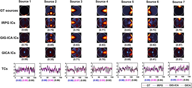
Individual ICs/TCs of one subject obtained from IRPG, GIG‐ICA, and GICA when the CNR of data was 0.5. Individual ICs obtained from IRPG, GIG‐ICA, and GICA are denoted by IRPG ICs, GIG‐ICA ICs, and GICA ICs, respectively. The value in parenthesis under each estimated IC is the relevant correlation coefficient between the IC and the GT source. The GT sources are also shown for comparison. The bottom row shows related TCs including the GT TCs denoted by red color, the TCs from IRPG denoted by blue color, the TCs from GIG‐ICA denoted by purple color, and the TCs from GICA denoted by black color. The correlation values under TCs from left to right correspond to IRPG, GIG‐ICA and GICA, respectively. Note that only the non‐artifact ICs/TCs are shown. [Color figure can be viewed in the online issue, which is available at http://wileyonlinelibrary.com.]

Using boxplots, we show the overall IC/TC accuracy of subjects under varying CNRs in Figure 6A,B, and display the results under different numbers of time points in Figure 6C,D. It is clear that the accuracy of the estimated ICs improved with increasing CNR or number of time points for all methods. Furthermore, measured by the mean of the overall IC accuracy across subjects, GIG‐ICA outperformed the other methods, particularly at low data quality and quantity. In terms of the accuracy of the obtained TCs, the increasing trend along the improved quality or quantity was not very apparent for all these methods, however, GIG‐ICA still showed relatively better results compared with the other methods.

Figure 6.

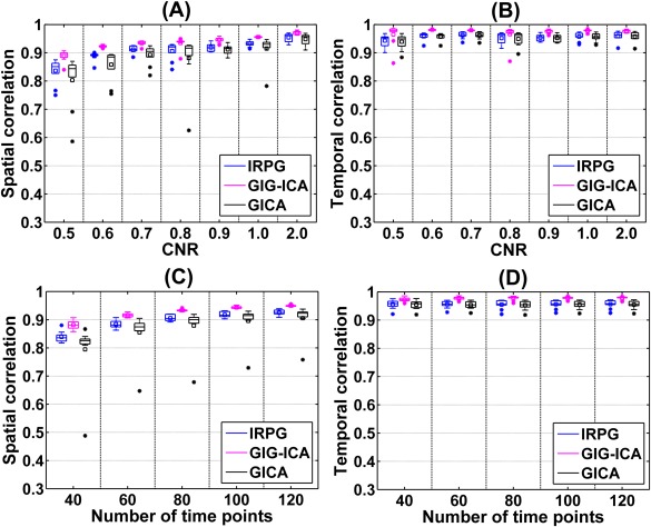
The overall IC/TC accuracy of subjects obtained from IRPG, GIG‐ICA, and GICA for datasets with different CNRs (A and B) or different numbers of time points (C and D). The x‐axis in each plot denotes CNR or number of time points. The y‐axis denotes each subject's overall spatial/temporal accuracy, obtained by averaging the correlations between the ground truth and the estimated ICs/TCs. Note that we only show the results of CNR = 0.5 to CNR = 1 and CNR = 2 due to the space limitation. For each boxplot, the central line is the median, and the edges of the box are the 25^th and 75^th percentiles. The whiskers extend to 1 inter‐quartile range, and the outliers are displayed with a “*” sign. The mean value is indicated by a square. Subsequent boxplots are formatted similarly. [Color figure can be viewed in the online issue, which is available at http://wileyonlinelibrary.com.]

In addition, for those datasets with different CNRs and different numbers of time points, the results from two‐tailed paired t‐tests demonstrate that the ICs/TCs accuracy of GIG‐ICA was significantly higher than that of IRPG (mean P value = 0.0043 and mean T value = 8.4216 for ICs accuracy; mean P value = 0.0034 and mean T value = 5.4457 for TCs accuracy), while the ICs/TCs accuracy of IRPG was significantly better than that of GICA (mean P value = 0.0215 and mean T value = 3.1939 for ICs accuracy; mean P value = 0.0416 and mean T value = 3.0302 for TCs accuracy). This is presumably due to the fact that GIG‐ICA performs independence optimization of components at the subject level, whereas IRPG and GICA focus only on group‐level independence.

As mentioned in the Materials and Methods section, we also investigated the performance of IRPG, which used regression to remove the individual subject artifacts. The summarized results of IRPG with regression‐based artifacts removal are included in Figure S4 of Supporting Information. The results of IRPG displayed in Supporting Information Figure S4 are almost identical to that presented in Figure 6 under the case of different CNRs, and are slightly worse than that presented in Figure 6 with respect to the temporal accuracy under the case of different numbers of time points. The possible reason is that ICA model based artifacts removal in IRPG may work better than regression‐based artifacts removal in simulations‐based experiments, due to that the simulations were generated based on typical ICA model.

Experiment 2: Effect of variable number of sources among subjects

The experiment investigated the performance of those methods using data with variable numbers of sources. As described above, we tested different model order ( $\mathrm{I}1$ in IRPG, $\mathrm{G}2$ in GIG‐ICA, and $\mathrm{A}2$ in GICA). Using boxplots, we show the overall IC/TC accuracy obtained from IRPG, GIG‐ICA, and GICA under different model order in Figure 7. Measured by the mean of overall IC/TC accuracy across subjects, GIG‐ICA showed the best performance, and in general IRPG had better performance than GICA.

Figure 7.

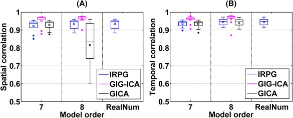
The overall IC/TC accuracy of subjects obtained from IRPG, GIG‐ICA, and GICA under different model order for datasets with different numbers of sources. The model order denotes parameter $\mathrm{I}1$ in IRPG, $\mathrm{G}2$ in GIG‐ICA, and $\mathrm{A}2$ in GICA. “RealNum” denotes the real number of sources in each subject (either 7 or 8). The y‐axis denotes each subject's overall spatial/temporal accuracy, obtained by averaging the correlations between the ground truth and the estimated ICs/TCs. [Color figure can be viewed in the online issue, which is available at http://wileyonlinelibrary.com.]

When the model order was set to 7, the results from paired t‐tests demonstrate that the ICs/TCs accuracy of GIG‐ICA was significantly higher than that of IRPG (P value = 0.0028 and T value = 3.1186 for ICs accuracy, P value = 0.0017 and T value = 3.2862 for TCs accuracy), but accuracy of IRPG had no significant difference with that of GICA (P value = 0.2534 and T value = −1.1535 for ICs accuracy, P value = 0.8476 and T value = 0.1930 for TCs accuracy). When the model order was specified as 8, the ICs accuracy of GIG‐ICA had significant higher values than that of IRPG (P value = 0.0037 and T value = 3.0254 for ICs accuracy, P value = 0.1769 and T value = 1.3668 for TCs accuracy), while the ICs accuracy of IRPG was significantly greater than that of GICA (P value = 3.33e‐6 and T value = 5.1350 for ICs accuracy, P value =0.6764 and T value = 0.4194 for TCs accuracy). When $\mathrm{I}1$ was set to $C$ (the real number of sources in each subject), IRPG obtained similar results to the case of $\mathrm{I}1$ = 8, since the artifact was accurately identified for each subject. It is worth noting that when $\mathrm{I}1$ was set to 8, the subject datasets with seven sources were decomposed into eight components including six non‐artifact ICs, one artifact IC, and one white‐noise‐like IC, thus the artifact IC can be identified correctly. However, when $\mathrm{I}1$ was set to 7, IRPG performed less well because the artifacts cannot be correctly removed from the subject datasets with eight sources.

Figure 7 also shows that GIG‐ICA had a reliable performance when $\mathrm{G}2$ was set to 7 and 8, indicating that GIG‐ICA still worked well when different subjects had different numbers of sources and the model order was slightly inaccurate. From this experiment, we also observe that GICA was more sensitive to model order than the other two methods, and the ICs accuracy of GICA was affected when $\mathrm{A}2$ was set to 8, since five subjects only had seven sources (a scenario where dual regression is known to perform poorly). Because the accurate number of components is very difficult to estimate correctly in practice, the relative insensitivity of GIG‐ICA to model order may provide an important benefit. The results relevant to IRPG with regression‐based individual‐subject artifacts removal are shown in Figure S5 of Supporting Information. The results shown in Supporting Information Figure S5 are very similar to that presented in Figure 7.

Experiment 3: Effect of spatially unique artifacts

In this experiment, we tested those methods using datasets with spatially unique artifact for each subject, and the artifacts were accurately identified for both IRPG and GIG‐ICA. Accuracy of each individual IC/TC of subjects is shown in Figure 8. The results show that even when subjects had spatially unique artifacts, GIG‐ICA had better performance for ICs (mean of ICs accuracy for IRPG and GIG‐ICA were 0.95 and 0.97, respectively) and a comparable performance for TCs compared with IRPG (mean of TCs accuracy for IRPG and GIG‐ICA were 0.9552 and 0.9554, respectively). Furthermore, both methods had better performance over traditional GICA without artifacts removal (mean of ICs and TCs accuracy for GICA were 0.85 and 0.94, respectively). Paired t‐tests results demonstrate that compared with IRPG, GIG‐ICA performed significantly better in ICs (P value = 0.0060 and T value = 2.8375 for ICs accuracy, P value = 0.9639 and T value = 0.0453 for TCs accuracy). Compared with GICA, the ICs/TCs accuracy of IRPG was significantly improved due to artifacts removal (P value = 5.82e‐5 and T value = 4.2845 for ICs accuracy; P value = 0.0001 and T value = 4.099 for TCs accuracy). In addition, the results of IRPG with regression‐based individual‐subject artifacts removal are shown in Figure S6 of Supporting Information, which are similar to that displayed in Figure 8.

Figure 8.

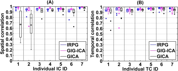
Spatial/temporal accuracy of each estimated IC/TC obtained from IRPG, GIG‐ICA, and GICA for datasets with unique artifacts. The x‐axis denotes the individual IC/TC ID with the same order as the first seven sources in Figure 2. The y‐axis denotes the spatial/temporal correlation between each subject‐specific IC/TC and the corresponding GT source/TC. [Color figure can be viewed in the online issue, which is available at http://wileyonlinelibrary.com.]

Experiments Using Resting‐State fMRI Data

Using test‐retest fMRI data, we compared the performance of IRPG, GIG‐ICA, and GICA. As described in the Experiments Using Resting‐State fMRI Data section, a classifier was trained to automatically identify individual‐subject artifacts in IRPG based on IC features. Training was performed with 1,125 individual ICs from scan 1, each with 249 features describing spatial, temporal, and spectral properties. Approximately half (49.1%) of these individual ICs were manually identified as artifacts. The optimal alpha and lambda parameters in the model [Sochat et al., 2014] were determined to be 0.13 and 0.0625, respectively, based on a maximum mean accuracy of 0.89 as achieved with 10‐fold cross validation. Given these parameters, the set of 249 possible features was reduced to 140 relevant features via sparsity constraints [Sochat et al., 2014], and the top 10 of which are listed in Table 3. The classifier was successful in distinguishing artifacts in training data (accuracy = 0.91, sensitivity = 0.91, specificity = 0.90) as well as unseen data (accuracy = 0.92, sensitivity = 0.95, specificity = 0.89) based on 270 individual ICs (45 ICs × 6 datasets) from scans 2 and scan 3 that were additionally labeled by the five raters. Using the trained classifier, 534 ICs (47.5%) and 515 ICs (45.8%) were identified as artifacts for scan 2 and scan 3, respectively. Within each subject, the number of non‐artifact individual ICs (out of 45) ranged from 16 to 32 (mean = 24, SD = 4).

Table 3.

The top 10 selected features and their relative weights

Feature	Weight
Percentage of total voxels in grey matter	0.35
The power of TC between 0.02 and 0.05 Hz	0.23
The number of activated voxels in Frontal_Sup_Medial_R	0.13
Power spectrum density of TC over 0.0671 HZ	0.13
Power spectrum density of TC over 0.0915 HZ	0.12
The number of activated voxels in Putamen_R	0.11
The number of activated voxels in Parietal_Sup_L	0.11
The number of activated voxels in Precuneus_R	0.11
Power spectrum density of TC over 0.0854 HZ	0.11
Power spectrum density of TC over 0.0488 HZ	0.10

In the following, we describe the performance of IRPG, GIG‐ICA, and GICA under the case of $\mathrm{I}3=15$, $\mathrm{G}2$ = 30, $\mathrm{A}2$ = 30 in detail, and then summarize the performance of these methods under different parameters.

Given $\mathrm{G}2$ = 30, 16 meaningful (non‐artifact) functional networks were found using GIG‐ICA. For IRPG and GICA, 15 and 30 components were obtained, respectively. Fourteen matched networks were finally identified across the three methods. One‐sample t‐tests (P < 0.01, FDR corrected) results of the 14 matched networks are displayed in Figure 9, which shows that the networks from those three methods are in general very similar. However, it seems that the T values for networks are larger in GIG‐ICA than that in the other two methods.

Figure 9.

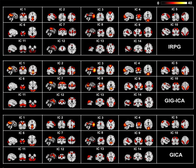
One‐sample t‐test T value maps for the matched networks in the case of $\mathrm{I}3$ = 15, $\mathrm{G}2$ = 30, $\mathrm{A}2$ = 30, thresholded at P < 0.01 with FDR correction for IRPG, GIG‐ICA, and GICA. [Color figure can be viewed in the online issue, which is available at http://wileyonlinelibrary.com.]

We show the correlation matrices of all individual ICs from IRPG, GIG‐ICA, and GICA in Figure 10. Each ICs consistency across the 75 datasets (25 participants with three scans) can be determined from a diagonal sub‐matrix (size: $75\times 75$). It can be observed from Figure 10 that the spatial correlations among corresponding subject‐specific ICs estimated by GIG‐ICA were relatively larger than those obtained with IRPG and GICA. Furthermore, many off‐diagonal lines parallel to the diagonal appeared in the correlation matrix for IRPG and GICA, indicating spatial correlations (or dependence) between different ICs from the same dataset. In addition, since GIG‐ICA explicitly optimizes the correspondence between individual networks and group ICs, it is not unexpected that it would perform better on this measure. However, based on the simulations above, we have found that GIG‐ICA does adapt to individual subject properties and this is also consistent with our initial publications [Du and Fan, 2011; Du and Fan, 2013]. We also observed some spatial correlations between components in GIG‐ICA. This appears to be due to the partial spatial overlap of components, reflecting the hierarchical division of a larger network into sub‐networks, as discussed in a previous study [Ma et al., 2011].

Figure 10.

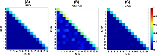
The correlation matrix between the matched individual networks from all 75 datasets for IRPG with $\mathrm{I}3$ = 15, GIG‐ICA with $\mathrm{G}2$ = 30, and GICA with $\mathrm{A}2$ = 30, respectively. Warmer color in blocks along the diagonal indicates spatial similarity between corresponding individual ICs. [Color figure can be viewed in the online issue, which is available at http://wileyonlinelibrary.com.]

As described above, for each matched network, we computed ICCs between the networks from scan 2 and the networks from scan 3, and then used the mean of ICC values in significant voxels (for all three methods) to reflect the short‐term reliability of this network. Similarly, the long‐term reliability of each matched network was computed based on ICCs between the networks from scan 1 and the averaged networks of scan 2 and scan 3. Figure 11A,B illustrate the short‐term and the long‐term reliability of each matched network obtained from the three methods. The results suggest that in general networks computed using GIG‐ICA were more reliable than those estimated with IRPG, and IRPG had improvement than traditional GICA in terms of some networks. Figure 11C,D show the intersubject effect variance between networks from scan 2 and networks from scan 3 as well as between networks from scan 1 and the averaged networks of scan 2 and scan 3. In terms of the intersubject effect variance, GIG‐ICA had greater values than IRPG, while IRPG showed higher values than GICA for most of networks.

Figure 11.

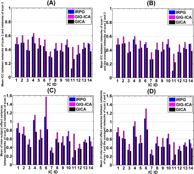
Reliability measurements of the matched networks obtained from IRPG with $\mathrm{I}3$ = 15, GIG‐ICA with $\mathrm{G}2$ = 30, and GICA with $\mathrm{A}2$ = 30. The x‐axis denotes the ID of the matched networks. (A) Short‐term reliability of networks. Each network's short‐term reliability was measured by mean of ICC values within significant voxels between networks from scan 2 and networks from scan 3. (B) Long‐term reliability of networks. Each network's long‐term reliability was measured by mean of ICC values within significant voxels between networks from scan 1 and the averaged networks of scan 2 and scan 3. (C) Mean of the variances of intersubject effect across significant voxels between networks from scan 2 and networks from scan 3. (D) Mean of the variances of intersubject effect across significant voxels between networks from scan 1 and the averaged networks of scan 2 and scan 3. [Color figure can be viewed in the online issue, which is available at http://wileyonlinelibrary.com.]

We also varied $\mathrm{I}3$, $\mathrm{G}2$, and $\mathrm{A}2$ to examine the influence of those parameters. As shown in Figure 12A,B, we compared the performances of those methods under different model order with respect to the short‐term and long‐term reliability of networks. Measured by the mean of ICC measures across networks, the reliability measures of GIG‐ICA were always higher than that of IRPG regardless of the used model order, and IRPG showed slight improvement than traditional GICA in our data. Figure 12C,D illustrate that measured by the mean of the intersubject effect variance measures across networks, GIG‐ICA had greater values than IRPG, while IRPG showed increased values than GICA. In addition, it seems like that the measures computed from traditional GICA were more sensitive to the used model order, compared with that estimated from the other two methods.

Figure 12.

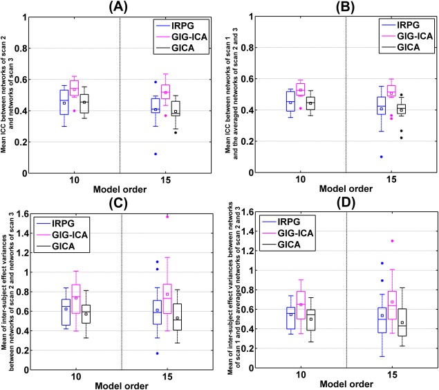
Reliability measurements of the matched networks obtained from IRPG, GIG‐ICA, and GICA under different model order. The x‐axis denotes $\mathrm{I}3$, $\mathrm{G}2$, or $\mathrm{A}2$. The y‐axis denotes each matched network's short‐term or long‐term reliability. (A) Short‐term reliability of networks. Each network's short‐term reliability was measured by mean of ICC values within significant voxels between networks from scan 2 and networks from scan 3. (B) Long‐term reliability of networks. Each network's long‐term reliability was measured by mean of ICC values within significant voxels between networks from scan 1 and the averaged networks of scan 2 and scan 3. (C) Mean of the variances of intersubject effect across significant voxels between networks from scan 2 and networks from scan 3. (D) Mean of the variances of intersubject effect across significant voxels between networks from scan 1 and the averaged networks of scan 2 and scan 3. [Color figure can be viewed in the online issue, which is available at http://wileyonlinelibrary.com.]

DISCUSSIONS AND CONCLUSION

In this article, we study and compare two approaches for artifacts removal in applying ICA on multi‐subjects’ fMRI data. One approach, recommended by the Human Connectome Project, which we call IRPG, is to remove artifact ICs from individual ICA results, and subsequently implement a traditional group ICA on cleaned data from all subjects. A second approach, named GIG‐ICA, identifies and removes group‐level artifacts after an ICA on all subjects’ datasets, and then estimates subject‐specific ICs with non‐artifact group ICs as spatial references. For comparison, we also assess traditional GICA to evaluate performance in the absence of artifacts removal. Using simulations, we evaluated those approaches with respect to the effects of data quality (CNR), data quantity (number of time points), variable source numbers across subjects, and presence of spatially unique artifacts. Furthermore, we investigated the performances of those methods using resting‐state test‐retest fMRI data with respect to the reliability of functional networks.

Simulations‐based experiments demonstrate that GIG‐ICA shows overall better performance than IRPG under the cases of different data quality and quantity, variable number of sources, and unique artifacts. Even when single‐subject artifacts removal is perfect for IRPG (as in Experiment 1, Experiment 3, and Experiment 2 when the model order was set to $C$) and subjects have spatially unique artifacts (as in Experiment 3), IRPG has a slightly worse performance, especially for estimation of ICs. Consistent with the conclusion reported in the Human Connectome Project, IRPG has improvement compared with traditional GICA, particularly in the cases of variable number of sources and unique artifacts, demonstrating the potential benefits of artifacts removal methods. The superiority of GIG‐ICA likely stems from identifying and removing artifacts at group level, which may be more robust than single‐subject decompositions, as well as the optimization of independence at the single‐subject level, which improves estimation accuracy of individual ICs. The reasonable performance of GIG‐ICA in conditions of low data quantity (Experiment 1) suggests that it may be an option for real‐time fMRI [Soldati et al., 2013]. The robustness of GIG‐ICA to the used model order and the variability of sources among subjects makes it a good option for large fMRI studies, which are likely to have heterogeneous datasets.

Evaluations using test‐retest fMRI data support our simulations‐based findings and suggest that GIG‐ICA can achieve functional networks with relatively higher reliability. In one sense this is expected, since GIG‐ICA explicitly optimizes the similarity of the individual subjects to the group reference components, however based on the simulations where GIG‐ICA also better matched the ground truth individual ICs, we think this is a desirable result that reflects more accurate estimation. In real application, artifact detection is often difficult because of the broad range of types of artifacts, the unknown pattern of artifacts, and the substantial intersubject variation. Furthermore, the uncertainty of sources number in real data can affect identification and removal of artifacts. In this article, we applied a supervised learning approach [Sochat et al., 2014] to identify artifacts, and achieved reasonably high accuracy. In recent work from the Human Connectome Project, a hierarchical fusion of classifiers was applied to identify the individual‐subject artifact ICs based on more than 180 features. The machine learning methods used here and elsewhere [Salimi‐Khorshidi et al., 2014; Smith et al., 2013] can mitigate the difficulties of single‐subject artifact detection in IRPG to a degree, however, manual identification for training data is still time consuming. Based on our simulations, even if this process were perfect, IRPG would not outperform GIG‐ICA.

The results presented in this article are subject to a number of limitations. (1) The simulations are relatively simple. Only one or two artifacts of eight sources were simulated, while the proportion of artifacts in fMRI data is certainly greater. Additionally, the spatial variability of simulated sources across subjects is relatively small. Since all of the group ICA methods evaluated assume similarity in the networks of interest, most sources were simulated by adding moderate subject‐specific variation to common templates. In real data, the variability across subjects could be much larger. We did simulate one case where each artifact was spatially unique across subjects (and thus highly variable) and results were consistent with our other simulations. However, we have not tested cases where the networks of interest are also extremely variable. It is important to note that all the evaluated group ICA methods assume similarity in the networks of interest, so the case where the functional networks are highly variable across subjects was not our main focus in this work. In addition, our recent work [Du et al., 2014b, 2015] also showed that GIG‐ICA can effectively investigate the group difference among similar diseases, such as schizophrenia, bipolar disorder, and schizoaffective disorder. (2) The number of sources in real data is unknown, therefore, we do not know the best dimensionality for artifact detection or ICA decompositions in general. Furthermore, we do not know the appropriate model order at which to compare these three methods in real data. We compared the three methods under different parameters, and found similar results for different values of $\mathrm{I}3$, $\mathrm{G}2$, and $\mathrm{A}2$, but it is possible that other model order would yield different performance for the methods. (3) The networks reliability measures used to assess performance in real data may be sensitive to (and favor) spatial similarity between ICs. While such measures could not be optimal, the use of networks reliability as proxies for assessing estimation quality is warranted in scenarios where the ground truth is unknown. The networks reliability are commonly used to evaluate ICA methods [Griffanti et al., 2014; Zuo et al., 2010]. (4) The detection and removal for artifacts was imperfect for real data, with ∼10% of ICs being mislabeled in this study, thus may unfairly reduce the performance of IRPG. However, our simulations‐based experiments illustrate that GIG‐ICA still had better performance than IRPG even when single‐subject artifacts removal in IRPG was perfect. The superiority of GIG‐ICA is likely due to the independence optimization of individual ICs.

The assumptions and biases of different group ICA approaches also need to be addressed. The IRPG approach cleans the data for each individual subject such that it hopefully coincides with the group ICA model. This is a reasonable approach, although the subject‐level artifacts removal can be time consuming and misclassification of individual artifacts can lead to additional error. In contrast, GIG‐ICA estimates subject‐level functional networks based on non‐artifact group ICs, while ignoring the variability of artifact sources. GIG‐ICA is slightly more flexible than IRPG in capturing individual subject maps due to the independence optimization of individual ICs. Both GIG‐ICA and IRPG appear to work better than not addressing the artifacts. Any of these approaches should be used with caution when applying to data with great variability, such as lesion or stroke data. The main advantage of group ICA is that it provides a group model to automatically link components across subjects. Single‐subject ICAs do not have this benefit and instead require a post‐hoc sorting approach. There are several alternative methods that have been proposed to perform functional network analysis of multiple subjects. Kim et al. [2012] incorporated sparsity into a dual regression method using a iterative algorithm. Schultz et al. [2014] proposed a template based rotation (TBR) method. Ma et al. [2013] proposed an independent vector analysis (IVA) based method. All these methods may provide potential benefits going forward.

In conclusion, we have evaluated three group ICA approaches including traditional GICA and two approaches with additional artifacts removal. Results show that both IRPG and GIG‐ICA show benefits over GICA, and GIG‐ICA shows additional improvements over IRPG in performance and implementation.

Supporting information

Supporting Information

REFERENCES

- Abou‐Elseoud A, Starck T, Remes J, Nikkinen J, Tervonen O, Kiviniemi V (2010): The effect of model order selection in group PICA. Hum Brain Mapp 31:1207–1216. [DOI] [PMC free article] [PubMed] [Google Scholar]
- Allen EA, Erhardt EB, Wei Y, Eichele T, Calhoun VD (2012): Capturing intersubject variability with group independent component analysis of fMRI data: A simulation study. Neuroimage 59:4141–4159. [DOI] [PMC free article] [PubMed] [Google Scholar]
- Baggio HC, Segura B, Sala‐Llonch R, Marti MJ, Valldeoriola F, Compta Y, Tolosa E, Junque C (2015): Cognitive impairment and resting‐state network connectivity in Parkinson's disease. Hum Brain Mapp 36:199–212. [DOI] [PMC free article] [PubMed] [Google Scholar]
- Beckmann C, Mackay C, Filippini N, Smith S (2009): Group comparison of resting‐state FMRI data using multi‐subject ICA and dual regression. Neuroimage 47(Suppl 1):S148. [Google Scholar]
- Beckmann CF, Smith SM (2005): Tensorial extensions of independent component analysis for multisubject FMRI analysis. Neuroimage 25:294–311. [DOI] [PubMed] [Google Scholar]
- Bell AJ, Sejnowski TJ (1995): An information‐maximization approach to blind separation and blind deconvolution. Neural Comput 7:1129–1159. [DOI] [PubMed] [Google Scholar]
- Calhoun VD (2001): fMRI activation in a visual‐perception task: Network of areas detected using the general linear model and independent components analysis. Neuroimage 14:1080–1088. [DOI] [PubMed] [Google Scholar]
- Calhoun VD, Adali T (2012): Multisubject independent component analysis of fMRI: A decade of intrinsic networks, default mode, and neurodiagnostic discovery. IEEE Rev Biomed Eng 5:60–73. [DOI] [PMC free article] [PubMed] [Google Scholar]
- Calhoun VD, Adali T, Pearlson GD, Pekar JJ (2001a): A method for making group inferences from functional MRI data using independent component analysis. Hum Brain Mapp 14:140–151. [DOI] [PMC free article] [PubMed] [Google Scholar]
- Calhoun VD, Adali T, Pearlson GD, Pekar JJ (2001b): Spatial and temporal independent component analysis of functional MRI data containing a pair of task‐related waveforms. Hum Brain Mapp 13:43–53. [DOI] [PMC free article] [PubMed] [Google Scholar]
- Calhoun VD, Liu J, Adali T (2009): A review of group ICA for fMRI data and ICA for joint inference of imaging, genetic, and ERP data. Neuroimage 45:S163–S172. [DOI] [PMC free article] [PubMed] [Google Scholar]
- Calhoun VD, Pekar JJ, Pearlson GD (2004): Alcohol intoxication effects on simulated driving: Exploring alcohol‐dose effects on brain activation using functional MRI. Neuropsychopharmacol 29:2097–2107. [DOI] [PubMed] [Google Scholar]
- De Martino F, Gentile F, Esposito F, Balsi M, Di Salle F, Goebel R, Formisano E (2007): Classification of fMRI independent components using IC‐fingerprints and support vector machine classifiers. Neuroimage 34:177–194. [DOI] [PubMed] [Google Scholar]
- Du YH, Allen EA, He H, Sui J, Calhoun VD (2014a): Brain functional networks extraction based on fMRI artifact removal: Single subject and group approaches. Conference proceedings: Annual International Conference of the IEEE Engineering in Medicine and Biology Society. IEEE Eng Med Biol Soc Annu Conf 2014:1026–1029. [DOI] [PubMed] [Google Scholar]
- Du YH, Fan Y (2011): Group information guided ICA for analysis of multi‐subject fMRI data. In: The 17th Annual Meeting of the Organization for Human Brain Mapping. Quebec City, Canada. June 26–30.
- Du YH, Fan Y (2013): Group information guided ICA for fMRI data analysis. Neuroimage 69:157–197. [DOI] [PubMed] [Google Scholar]
- Du YH, Li HM, Wu H, Fan Y (2012): Identification of subject specific and functional consistent ROIs using semi‐supervised learning. Proceedings of SPIE, Medical Imaging 2012: Image Processing. San Diego, SPIE, pp 8314.
- Du YH, Liu JY, Sui J, He H, Pearlson GD, Calhoun VD (2014b): Exploring difference and overlap between schizophrenia, schizoaffective and bipolar disorders using resting‐state brain functional networks. In: The 36th Annual International Conference of the IEEE Engineering in Medicine and Biology Society (EMBC). Chicago, IEEE, pp 1517–1520. [DOI] [PubMed]
- Du YH, Pearlson GD, Liu J, Sui J, Yu QB, He H, Castro E, Calhoun VD (2015): A group ICA based framework for evaluating resting fMRI markers when disease categories are unclear: Application to schizophrenia, bipolar, and schizoaffective disorders. Neuroimage 122:272–280. [DOI] [PMC free article] [PubMed] [Google Scholar]
- Erhardt EB, Allen EA, Wei Y, Eichele T, Calhoun VD (2012): SimTB, a simulation toolbox for fMRI data under a model of spatiotemporal separability. Neuroimage 59:4160–4167. [DOI] [PMC free article] [PubMed] [Google Scholar]
- Erhardt EB, Rachakonda S, Bedrick EJ, Allen EA, Adali T, Calhoun VD (2011): Comparison of multi‐subject ICA methods for analysis of fMRI data. Hum Brain Mapp 32:2075–2095. [DOI] [PMC free article] [PubMed] [Google Scholar]
- Esposito F, Scarabino T, Hyvarinen A, Himberg J, Formisano E, Comani S, Tedeschi G, Goebel R, Seifritz E, Di Salle F (2005): Independent component analysis of fMRI group studies by self‐organizing clustering. Neuroimage 25:193–205. [DOI] [PubMed] [Google Scholar]
- Filippini N, MacIntosh BJ, Hough MG, Goodwin GM, Frisoni GB, Smith SM, Matthews PM, Beckmann CF, Mackay CE (2009): Distinct patterns of brain activity in young carriers of the APOE‐epsilon4 allele. Proc Natl Acad Sci USA 106:7209–7214. [DOI] [PMC free article] [PubMed] [Google Scholar]
- Greicius MD, Srivastava G, Reiss AL, Menon V (2004): Default‐mode network activity distinguishes Alzheimer's disease from healthy aging: Evidence from functional MRI. Proc Natl Acad Sci USA 101:4637–4642. [DOI] [PMC free article] [PubMed] [Google Scholar]
- Griffanti L, Salimi‐Khorshidi G, Beckmann CF, Auerbach EJ, Douaud G, Sexton CE, Zsoldos E, Ebmeier KP, Filippini N, Mackay CE, Moeller S, Xu J, Yacoub E, Baselli G, Ugurbil K, Miller KL, Smith SM (2014): ICA‐based artefact removal and accelerated fMRI acquisition for improved resting state network imaging. Neuroimage 95:232–247. [DOI] [PMC free article] [PubMed] [Google Scholar]
- Guo CC, Kurth F, Zhou J, Mayer EA, Eickhoff SB, Kramer JH, Seeley WW (2012): One‐year test‐retest reliability of intrinsic connectivity network fMRI in older adults. Neuroimage 61:1471–1483. [DOI] [PMC free article] [PubMed] [Google Scholar]
- Himberg J, Hyvarinen A, Esposito F (2004): Validating the independent components of neuroimaging time series via clustering and visualization. Neuroimage 22:1214–1222. [DOI] [PubMed] [Google Scholar]
- Jarrahi, B , Mantini, D , Balsters, JH , Michels, L , Kessler, TM , Mehnert, U , Kollias, SS (2015): Differential functional brain network connectivity during visceral interoception as revealed by independent component analysis of fMRI time‐series. Hum Brain Mapp 36:4438–4468. [DOI] [PMC free article] [PubMed] [Google Scholar]
- Kim YH, Kim J, Lee JH (2012): Iterative approach of dual regression with a sparse prior enhances the performance of independent component analysis for group functional magnetic resonance imaging (fMRI) data. Neuroimage 63:1864–1889. [DOI] [PubMed] [Google Scholar]
- Kundu P, Inati SJ, Evans JW, Luh WM, Bandettini PA (2012): Differentiating BOLD and non‐BOLD signals in fMRI time series using multi‐echo EPI. Neuroimage 60:1759–1770. [DOI] [PMC free article] [PubMed] [Google Scholar]
- Lee JH, Lee TW, Jolesz FA, Yoo SS (2008): Independent vector analysis (IVA): multivariate approach for fMRI group study. Neuroimage 40:86–109. [DOI] [PubMed] [Google Scholar]
- Li YO, Adali T, Calhoun VD (2007): Estimating the number of independent components for functional magnetic resonance imaging data. Hum Brain Mapp 28:1251–1266. [DOI] [PMC free article] [PubMed] [Google Scholar]
- Ma S, Correa NM, Li XL, Eichele T, Calhoun VD, Adali T (2011): Automatic identification of functional clusters in FMRI data using spatial dependence. IEEE Trans Biomed Eng 58:3406–3417. [DOI] [PMC free article] [PubMed] [Google Scholar]
- Ma S, Phlypo R, Calhoun VD, Adali T (2013): Capturing group variability using IVA: A simulation study and graph‐theoretical analysis. Int Conf Acoust Speech 3128–3132. [Google Scholar]
- McKeown MJ, Makeig S, Brown GG, Jung TP, Kindermann SS, Bell AJ, Sejnowski TJ (1998): Analysis of fMRI data by blind separation into independent spatial components. Hum Brain Mapp 6:160–188. [DOI] [PMC free article] [PubMed] [Google Scholar]
- Moritz CH, Rogers BP, Meyerand ME (2003): Power spectrum ranked independent component analysis of a periodic fMRI complex motor paradigm. Hum Brain Mapp, 18:111–122. [DOI] [PMC free article] [PubMed] [Google Scholar]
- Perlbarg V, Bellec P, Anton JL, Pelegrini‐Issac M, Doyon J, Benali H (2007): CORSICA: Correction of structured noise in fMRI by automatic identification of ICA components. Magn Reson Imaging 25:35–46. [DOI] [PubMed] [Google Scholar]
- Salimi‐Khorshidi G, Douaud G, Beckmann CF, Glasser MF, Griffanti L, Smith SM (2014): Automatic denoising of functional MRI data: Combining independent component analysis and hierarchical fusion of classifiers. Neuroimage 90:449–468. [DOI] [PMC free article] [PubMed] [Google Scholar]
- Schopf V, Kasess CH, Lanzenberger R, Fischmeister F, Windischberger C, Moser E (2010): Fully exploratory network ICA (FENICA) on resting‐state fMRI data. J Neurosci Methods 192:207–213. [DOI] [PubMed] [Google Scholar]
- Schultz AP, Chhatwal JP, Huijbers W, Hedden T, van Dijk KR, McLaren DG, Ward AM, Wigman S, Sperling RA (2014): Template based rotation: A method for functional connectivity analysis with a priori templates. Neuroimage 102(Pt 2):620–636. [DOI] [PMC free article] [PubMed] [Google Scholar]
- Smith SM, Beckmann CF, Andersson J, Auerbach EJ, Bijsterbosch J, Douaud G, Duff E, Feinberg DA, Griffanti L, Harms MP, Kelly M, Laumann T, Miller KL, Moeller S, Petersen S, Power J, Salimi‐Khorshidi G, Snyder AZ, Vu AT, Woolrich MW, Xu J, Yacoub E, Ugurbil K, Van Essen DC, Glasser MF; Consortium WUMH (2013): Resting‐state fMRI in the Human Connectome Project. Neuroimage 80:144–168. [DOI] [PMC free article] [PubMed] [Google Scholar]
- Smith SM, Beckmann CF, Ramnani N, Woolrich MW, Bannister PR, Jenkinson M, Matthews PM, McGonigle DJ (2005): Variability in fMRI: a re‐examination of inter‐session differences. Hum Brain Mapp 24:248–257. [DOI] [PMC free article] [PubMed] [Google Scholar]
- Sochat V, Supekar K, Bustillo J, Calhoun V, Turner JA, Rubin DL (2014): A robust classifier to distinguish noise from FMRI independent components. PLoS One 9:e95493 [DOI] [PMC free article] [PubMed] [Google Scholar]
- Soldati N, Calhoun VD, Bruzzone L, Jovicich J (2013): ICA analysis of fMRI with real‐time constraints: An evaluation of fast detection performance as function of algorithms, parameters and a priori conditions. Front Hum Neurosci 7:1–11. [DOI] [PMC free article] [PubMed] [Google Scholar]
- Svensen M, Kruggel F, Benali H (2002): ICA of fMRI group study data. Neuroimage 16:551–563. [DOI] [PubMed] [Google Scholar]
- Tohka J, Foerde K, Aron AR, Tom SM, Toga AW, Poldrack RA (2008): Automatic independent component labeling for artifact removal in fMRI. Neuroimage 39:1227–1245. [DOI] [PMC free article] [PubMed] [Google Scholar]
- van de Ven V, Bledowski C, Prvulovic D, Goebel R, Formisano E, Di Salle F, Linden DE, Esposito F (2008): Visual target modulation of functional connectivity networks revealed by self‐organizing group ICA. Hum Brain Mapp 29:1450–1461. [DOI] [PMC free article] [PubMed] [Google Scholar]
- Zuo XN, Kelly C, Adelstein JS, Klein DF, Castellanos FX, Milham MP (2010): Reliable intrinsic connectivity networks: test‐retest evaluation using ICA and dual regression approach. Neuroimage 49:2163–2177. [DOI] [PMC free article] [PubMed] [Google Scholar]
Associated Data
This section collects any data citations, data availability statements, or supplementary materials included in this article.
Supplementary Materials