Computer-Aided Assessment of Breast Density: Comparison of Supervised Deep Learning and Feature-Based Statistical Learning

Abstract

Breast density is one of the most significant factors that are associated with the cancer risk. In this study, our purpose was to develop a supervised deep learning approach for automated estimation of percentage density (PD) on digital mammograms (DM). The input “for processing” DM was first log-transformed, enhanced by a multi-resolution preprocessing scheme, and subsampled to a pixel size of 800μm×800μm from 100μm×100μm. A deep convolutional neural network (DCNN) was trained to estimate a probability map of breast density (PMD) by using a domain adaptation resampling method. The PD was estimated as the ratio of the dense area to the breast area based on the PMD. The DCNN approach was compared to a feature-based statistical learning approach. Gray level, texture and morphological features were extracted and least absolute shrinkage and selection operator (LASSO) was used to combine the features into a feature-based PMD. With approval of the Institutional Review Board, we retrospectively collected a training set of 478 DMs and an independent test set of 183 DMs from patient files in our institution. Two experienced Mammography Quality Standards Act (MQSA) radiologists interactively segmented PD as the reference standard. Ten-fold crossvalidation was used for model selection and evaluation with the training set. With crossvalidation, DCNN obtained a Dice’s coefficient (DC) of 0.79±0.13 and Pearson’s correlation (r) of 0.97 whereas feature-based learning obtained DC=0.72±0.18 and r=0.85. For the independent test set, DCNN achieved DC=0.76±0.09 and r=0.94 while feature-based learning achieved DC=0.62±0.21 and r=0.75. Our DCNN approach was significantly better and more robust than the feature-based learning approach for automated PD estimation on DMs, demonstrating its potential use for automated density reporting as well as for model-based risk prediction.

I. INTRODUCTION

Breast cancer is one of the leading causes of death among women (Lauby-Secretan et al 2015). The American Cancer Society estimates there will be about 252,710 new cases of invasive breast cancer to be diagnosed in women, about 40,610 deaths and about 63,410 new cases of carcinoma in situ to be diagnosed in the United States in 2017 (Siegel et al 2017). Early detection of breast cancer has strong impact on patient survival. Screening mammography is the most effective and low-cost method to date for early cancer detection. Mammographic breast density has been proven to be a strong factor for cancer risk prediction (Wolfe 1976, Kerlikowske 2007, Vachon et al 2007), with risk estimates 4 to 6 folds greater for women in the highest quartile of density (≥75%) than women with the least dense breasts (<5%) (McCormack and dos Santos Silva 2006, Boyd et al 2007). A recent population study in the US concluded that breast density was the most prevalent risk factor for both pre- and post-menopausal women and had the largest effect on the population-attributable risk proportion of breast cancer (Engmann et al 2017).

More than twenty states in the US have passed the breast density notification law, which requires radiologists to inform patients with high breast density. In clinical practice, radiologists assign the breast density category following the BI-RADS lexicon (2013) by subjective visual judgement of the fibroglandular tissue displayed on mammograms. A simple predictive model for breast cancer risk (Tice et al 2005), based on the BI-RADS category alone adjusted for age and ethnicity, was found to be as accurate as the Gail model. However, the assignment of density categories with qualitative approaches yields large inter- and intra-observer variabilities among radiologists (kappa statistics 0.43) (Berg et al 2000, Martin et al 2006). In addition, an automated quantitative estimate of breast density may be more suitable to be incorporated into risk prediction models to stratify cancer risk and to promote risk-based screening and targeted prevention.

The percentage of dense area (PD) on mammograms is the most commonly used quantitative descriptor to measure the relative amount of fibroglandular tissue in the breast. Wolfe et al. (Wolfe et al 1987, Saftlas et al 1991) developed a planimetry method to measure the area of dense tissue relative to the breast area by manually tracing around the regions of dense tissue on mammograms. Another approach was to interactively select threshold gray level to segment the dense areas on a mammogram (Byng et al 1994, Boyd et al 1995). Planimetry or interactive thresholding of PDA are straightforward to perform, but often labor intensive and involves subjective operator decisions. Zhou et al. (Zhou et al 2001) developed an automated method for quantitative PD estimation based on a gray-level histogram classification technique, and the correlation of the estimated PD with the percentage of volumetric breast density was studied by using mammograms and breast MR images of the same patients (Wei et al 2004). For 67 CC views, the correlation between the computer-estimated PD and the PD by radiologists was 0.91. Highnam et al. (Highnam and Brady 1999, Highnam et al 2006) developed a computerized method for the estimation of a quantitative representation of the volume of non-fat tissue and breast density on mammograms, which they called the standard mammogram form (SMF). A later study (Zoe Aitken 2010) found that the correlation between the percentage of SMF and the percentage density by interactive thresholding was low (Spearman correlation coefficient = 0.68). Keller et al. used the thresholding method to process the images and proposed an algorithm based on adaptive multiclass fuzzy c-means clustering and a support vector machine (SVM) classifier (Keller et al 2012). Their results showed that the Pearson product-moment correlation coefficient between algorithm-estimated and radiologist-estimated per-breast PD was 0.82 (CI: 0.76-0.86) in raw images and 0.85 (CI: 0.80-0.89) in processed images. Oliver et al. (Oliver et al 2015) developed a learning approach in which textural and morphological features were combined with an SVM for dense pixel classification. They compared the PD with the BI-RADS category of the mammograms, and found that BI-RADS I: 0.20±0.08, BI-RADS II: 0.32±0.09, BI-RADS III: 0.47±0.10, BI-RADS IV: 0.58±0.13.

Commercial software for quantitative estimation of volumetric breast density became available in recent years. A study (Brandt et al 2015) found that the difference between two commonly used commercial software and the BI-RADS density categories by radiologists could be as large as 14% in the classification of women with dense breasts, and the overall agreement measured by weighted kappa statistics was moderate (0.4 < kappa < 0.6). The large variations in breast density estimates by different methods may lead to substantial effects when density is used for risk-based cancer screening.

Recently, deep convolution neural network (DCNN) has been shown to be particularly successful in the field of computer vision (Krizhevsky et al 2012, Szegedy et al 2016). CNN has been used for computer-aided cancer detection in medical imaging since early 90s (Chan et al 1993, Lo et al 1993, Chan et al 1995, Lo et al 1995a, Lo et al 1995b, Sahiner et al 1996). The recent rise of its use in computer vision field can be attributed to the dramatic increase in computational power using graphic processing units and training with big data while reducing overfitting with new regularization and activation methods that enable the use of very complex CNN structures, resulting in improved learning capability (Goodfellow et al 2016). A survey of the application of DCNN in medical image analysis can be found in (Litjens et al 2017). In comparison to statistical learning approaches, DCNN has two major differences: 1) its convolution neurons, which are inspired by the structure of the mammalian visual system (Hubel and Wiesel 1959), is suitable for vision feature extraction; and 2) its deep network architecture plus back-propagation optimization are capable of learning more complex representation of large amount of visual features.

In this study, we constructed a DCNN for estimation of breast density on full-field digital mammograms (DM). Our DCNN was trained to classify mammographic pixels into fatty class or dense class. A probability map of breast density (PMD) for a given DM was generated and compared to radiologists’ interactive thresholding segmentation. In comparison, we also developed a statistical learning method, in which breast parenchyma features designed with domain knowledge were extracted and then combined with least absolute shrinkage and selection operator (LASSO) regression for PMD estimation.

II. MATERIALS AND METHOD

2.1 Data Set

With approval of the Institutional Review Board, we retrospectively collected 661 DMs from patient files at our institution. Our data set was collected in two stages due to the time constraint to establish the reference standard, in which two Mammography Quality Standards Act (MQSA) qualified radiologists segmented the dense regions on each DM by interactive thresholding. In stage I, we collected 478 DMs from 352 patients for training of our computer methods. We then continued to collect another 183 DMs from 92 patients for independent testing in stage II. Only the craniocaudal (CC) views of each case were used in this study. All DMs were acquired with GE Senographe DM systems between 2001 to 2016. The GE system has a CsI phosphor/a:Si active matrix flat panel digital detector with a pixel size of 100 μm × 100 μm and the images are stored at 16 bits per pixel. In general, DMs are preprocessed with proprietary methods by the manufacturer before being displayed to radiologists in clinical practice. In our institution, both “for processing” and “for presentation” DMs were routinely archived in the patient picture archiving and communication system.

The pixel value in the “for processing” DM has a linear relationship with the x-ray exposure incident on the detector while the “for presentation” DM depends on the specific vendor’s proprietary image processing algorithms. Computer vision techniques trained to extract information from the images are likely to be sensitive to the preprocessing method to some degrees. We used the “for processing” DMs as input to develop and validate the methods in order to develop a system that is less dependent on the DM manufacturer’s processing method.

The “for processing” (raw) DM first underwent logarithmic transform and a two-step boundary detection for automated breast area segmentation, in which Otsu’s method (Otsu 1979) was used to binarize the image approximately into pixels interior and exterior to the breast. An 8-connectivity labeling method was used to identify the connected components on the image. The breast region was identified as the largest components on DM. The Laplacian pyramid method (Burt and Adelson 1983, Wei et al 2005) was then used to decompose the log-transformed DM into multi-scales. Our previously designed nonlinear weight function (Wei et al 2005) that adaptively determined the local weights based on the pixel gray level from each of the low-pass components was used to enhance the high-pass components. The processed DM image was recomposed by summing the weighted components and used for subsequent image analysis. This approach of including image preprocessing as an integral part of the image analysis tool makes it more robust against the variabilities in image preprocessing methods among different manufacturers’ systems and the changes over time even within the same manufacturer’s system.

To establish a reference standard, two experienced MQSA radiologists visually assessed the BI-RADS density categories and segmented the dense regions by interactive thresholding for each DM processed with our multiscale method. We used an in-house developed graphical user interface (GUI), which allowed windowing of the displayed image, for interactive thresholding and recording the BI-RADS density categories and the gray level threshold. PD was calculated as the ratio of dense area to breast area. The average of the PDs from the two radiologists was used as the reference standard for the supervised training and evaluation of our automated segmentation methods.

2.2 PD Estimation

Figure 1 illustrates the image analysis process in our automated breast density segmentation and estimation tool. The purpose of this process is to separate the breast region into 2 parts, the dense region and the fatty region. For a given pixel on DM, we extracted a region of interest (ROI) centered at this pixel and train our models with supervised learning methods to classify the pixel as dense or fatty. Since the adjacent pixels were correlated, we used sparse sampling to reduce redundancy, in which a non-overlapping moving window of 3 × 3 pixels was panned over the breast region. The central pixels of the moving windows were used as the centers of image patches, each of size K × K pixels, to be extracted for the training of the models. The patch size K for the DCNN was chosen by comparing the DCNN performance in a range of K values, as detailed in the following sections. The output of the prediction model is the probability that the central pixel of an input image patch belongs to the dense class.

Figure 1.

The flow diagram of our image analysis tool for automated estimation of the percentage of breast density (PD) using model-based prediction. The model is either a DCNN model or a feature-based model. When the trained image analysis tool is applied to a DM for testing, all pixels on the DM is processed without spare sampling.

With sparse sampling, we generated 968,264 image patches from 478 DMs. The label of each image patch was determined by the central pixel of the patch whether it was in the dense class (labeled as 1) or the fatty class (labeled as 0) in the binarized DM from radiologists’ interactive thresholding.

2.2.1 Deep Convolutional Neural Network (DCNN)

A convolutional neural network (CNN) is designed to process data that has a grid-like topology. CNN has been successful in computer vision problems. Convolution is a mathematical operation that can be written as an integral transformation:

$$[f\ast g](t)={\displaystyle \int f(\tau )}g(t-\tau )d\tau$$

where f is an input signal and g is a convolutional kernel. In machine learning application, one can consider the output of a convolution operation as the feature map of the input signal f through an integral transformation by a convolutional kernel g the weights of which are determined by training. Traditional neural network uses matrix multiplication to describe the interaction between each input unit and each output unit. With convolution, CNN enables sparse interactions and parameter sharing of input and output units. This is particularly useful in computational efficiency when the network is deep.

Figure 2 show the detailed architecture of our DCNN for PD estimation. The network contained six stages: the first three stages as feature generator and the second three stages as probability predictor. In the feature generator, each of stages S1 and S2 consisted of a convolutional layer, a rectified linear unit (ReLU) activation layer, a max pooling layer and a normalization layer; S3 consisted of a convolutional layer, a ReLU activation layer and a max pooling layer. The probability predictor was composed of three fully connected layers with a ReLU activation between adjacent layers. The output of the last fully connected layer was fed to a 2-way softmax classifier to generate the probability of the central pixel of the image patch being dense or fatty. A dropout layer (Hinton et al 2012) was used to connect the feature generator and the probability predictor to prevent overfitting.

Figure 2.

Architecture of deep convolutional neural network (DCNN) for breast density estimation. Upper: the DCNN’s input is 3721-dimensional, and the number of neurons in the network’s hidden layers is given by 69,984—15,488—2304—256—128—2; Left: the detailed DCNN structure.

In the feature generator, a non-saturating and nonlinear activation function ReLU: f(x) = max(0, x) was used after each convolutional layer due to its faster and effective training in deep network structure (Nair and Hinton 2010). The pooling layer reduced the number of parameters and the amount of computation with a non-linear subsampling approach and was also useful for controlling overfitting. The local response normalization (LRN) layers implemented the lateral inhibition that would normalize the unbounded activations from the ReLU neurons (Krizhevsky et al 2012). The normalization would enhance the response of neurons with high activation relative to those of the neighboring neurons, and thus increasing the relative response of signals.

During DCNN training, the network was optimized by stochastic gradient descent with the training set of K × K -pixel patches. In each training epoch, the training set was randomly divided into mini batches as input to the DCNN and N_I iterations (N_I = number of training samples/mini batch size) were performed within each epoch. The optimization was to minimize the cross entropy between the empirical distribution (reference standard provided by radiologists) defined by the training set and that estimated by the DCNN model. With the empirical distribution as P_i and the model estimated distribution as Q_i, for class i, the cross entropy loss over the same random variable x_j in one mini batch can be defined as

$$J_{\theta }=-\frac{1}{m}\left[{\displaystyle {\sum }_{j=1}^m{P}_i(x_j)}\mathit{log}{Q}_i(x_j)\right]+\alpha R(\theta )$$

where θ was the parameters in the model, R(θ) was the regularization term, and m was the number of samples in a mini batch. In this study, we used L2 norm as the regularization.

After training, image patches centered pixel by pixel on the DM were fed into the trained DCNN. The output score of the DCNN for each patch provides an estimate of the probability of the center pixel being dense, thus generating the PMD of the DM for the final density segmentation. By selecting a threshold on the probability of a pixel being fatty or dense, the PMD was segmented into a binary image and the PD was calculated as the ratio of total number of dense pixels above the threshold relative to the total number of pixels in the breast area.

2.2.2 Feature-based Statistical learning

Feature-based statistical learning methods have been used for breast density estimation in previous studies. To compare with the DCNN approach, we developed a statistical learning approach using features designed with domain knowledge for the same classification task as that for the DCNN, in which a given pixel was classified into one of the two classes (dense or fatty). We extracted 137 features for each pixel consisting of 3 types of features: 1) intensity, 2) texture, and 3) morphological. Table 1 summarized the features and the parameters. We chose these features based on their usefulness demonstrated in previous studies (Keller et al 2012, Arefan et al 2015, Oliver et al 2015) for the same or similar tasks. We used LASSO, which is a regression analysis method that performs both variable selection and regularization, to combine the features and to generate the PMD. In LASSO, the problem is to solve a regularized linear model with L1 norm. The optimization function of LASSO is defined as:

$$\underset{{\beta }_0,\beta }{min}(\frac{1}{N}{\displaystyle \sum _{i=1}^N{\Vert y_i-{\beta }_0-x_i^T\beta \Vert }_2^2+\lambda {\Vert \beta \Vert }_1)}$$

where y_i is the target function, x_i is the observation, β₀ and β are the model parameters, λ is a non-negative regularization parameter and N is the number of training samples.

Tabel 1.

Feature set for feature-based learning. Different window sizes were used in texture and morphologic feature extraction. The position operator: (direction, distance in pixels) of (0°,2), (45°,2) were used for co-occurrence matrix.

Type	Feature	Window size (pixels)
Gray level	Processed image
	Log-transformed image
	Adaptive-histogram image
	Histogram-equalization image
	Moment-order-1	11, 21, 31, 41,51,61,71,81
	Moment-order-2	11, 21, 31, 41,51,61,71,81
	Moment-order-3	11, 21, 31, 41,51,61,71,81
	Skewness	11, 21, 31, 41,51,61,71,81
	Kurtosis	11, 21, 31, 41,51,61,71,81
	Entropy	11, 21, 31, 41,51,61,71,81
Texture	Energy	(0°,2), (45°,2) 11, 21, 31, 41,51,61,71,81
(Co-occurrence Matrices)	Contrast	(0°,2), (45°,2) 11, 21, 31, 41,51,61,71,81
	Correlation	(0°,2), (45°,2) 11, 21, 31, 41,51,61,71,81
	Homogeneity	(0°,2), (45°,2) 11, 21, 31, 41,51,61,71,81
	Entropy	(0°,2), (45°,2) 11, 21, 31, 41,51,61,71,81
Morphologic	Distance to skin line
	Pixel location related to the nipple location
	Breast size
	Perimeter length

2.3 Model Selection and Evaluation

We collected two data sets for training and independent testing. The training set was used for model building. The test set was used for independent evaluation after all parameters and weights by DCNN and feature-based learning were fixed. In the rest of this section, we described the model selection and evaluation during the training process.

We used 10-fold cross validation for model selection. We randomly separated the training set into 10 folds. After training with nine folds was completed, the parameters and all weights were fixed and applied to the remaining fold for validation. The receiver operating characteristic (ROC) analysis was applied to the output score of the image patches, using the class labels of the central pixels of the patches as the truth. The classification accuracy was assessed with the area under the ROC curve (AUC) for each validation fold. A specific model that yielded the smallest error (in our case the highest average AUC) from the 10 validation folds was used. The 10-fold cross validation was chosen because it has been shown empirically to yield test error estimates that can avoid both excessively high bias and very high variance (Hastie et al 2011).

Our training set was unbalanced in PD distribution. Figure 3 illustrated the distribution of interactive PDs according to radiologist’s BI-RADS rating in the training set. The PDs in the training set ranged from 0.7% to 83.1% (mean value: 24.0%±19.5%). 54.8% (262/478) of the images in the training set had density less than 20%. To alleviate this problem, we used a domain adaptation method during the model selection. The training objective of DCNN was to reach a stable state by updating the model parameters iteratively. During the DCNN training, the model parameters were updated in each mini-batched sample, which was randomly drawn from the training samples. Driven by the significance of the depth in DCNN training, the notorious problem of vanishing/exploding gradients is aggravated due to the differences in the sample distribution among different mini-batches. Let the random training set be T and a preferred balanced data set be D which was a subset of T, the learning objective was to build a model that could obtain high predictive accuracy on T based on D. Our domain adaptation strategy was to resample the training data T based on its PD to approximate the distribution of D. In this study, we compared the regular resampling to that with domain adaptation strategy:

1. Regular cross-validation

   Random separation of the entire data set into 10 folds. At each cross-validation, select one fold as the test set, the remaining 9 folds as the training data set.

2. Cross-validation with domain adaptation strategy

   In our training set, 54.8% of images (262 out of 478 images) had a PD less than 0.2. To reduce the low PD images, we empirically chose a hyperparameter, t_PD, the threshold on the PD values, to be 0.2. The images with PD < t_PD were then randomly split into two subsets of 131 images each. The revised training set was the reduced image set composed of only one set of images with PD < 0.2 and the rest of the images with PD ≥ 0.2. The revised training set was used for 10-fold cross-validation. The remaining 131 images with PD < 0.2 were also randomly separated into 10 folds and only used for validation. At each cross-validation, 9 folds of the revised training set were used to train the model, and one fold of the revised training set and one fold of the 131 images with PD < 0.2 were used for validation.

Figure 3.

The distribution of percentage of breast density (PD) with respect to BI-RADS density categories in the training set. For the training set of 478 DMs, the numbers of images in the four BI-RADS categories were 108, 169, 124, and 77, respectively.

Figure 4 shows the distribution of the number of images as a function of PDs for the two resampling methods.

Figure 4.

Distribution of the number of images in the training set as a function of percentage of breast density (PDs) for the two resampling methods. Regular cross validation: 478 images; Domain adaptation resampling: 347 images.

We compared the segmentation of dense areas by the machine learning approaches with the reference standard. The DCNN output a classification score ranging from 0 to 1 for each pixel on the DM, thereby generating a PMD. A threshold of 0.5 was applied to the PMD to obtain a binarized image. The Dice coefficient (Dice 1945) that measured the overlap of the dense areas between the computer segmentation and the reference standard and the Pearson’s correlation coefficient of the PD values were calculated to assess the similarity of the segmentations by the DCNN and the feature-based method relative to that of the radiologists. In addition, the true positive (TP) rate for a given image was calculated as the number of TP pixels relative to the total number of dense pixels in the reference standard for that image, where a TP pixel was defined as a computer-segmented pixel that overlapped with a dense pixel in the reference standard. Both the Dice coefficient and the TP rate were calculated for individual images and then averaged over all images in a given data set. A two-tailed paired t-test was performed to examine the significance in the differences between the two machine learning methods and the radiologists.

III. RESULTS

The DCNN was trained by mini-batch stochastic gradient descent. The size of a mini-batch for stochastic gradient descent was 128. The learning rate was initialized at 10⁻³, and reduced by a factor of 0.8 after every 10,000 training iterations. Using the architecture in Figure 2, we compared three different patch sizes (K): 41 pixels (3.28 cm), 61 pixels (4.88 cm), and 81 pixels (6.48 cm). The average validation AUCs over 10 folds were 0.906±0.006, 0.981±0.003, and 0.630 ±0.084, respectively. We therefore chose a patch size of 61 pixels (4.88 cm) for final comparison with feature-based learning.

Figure 5 showed the variations in the validation AUCs during the DCNN training for the two resampling methods. After about 5,000 iterations, the training with domain adaptation stabilized and reached an average validation AUC of 0.981±0.003. The training with regular resampling did not converge even after 270,000 iterations. We therefore used the DCNN model trained with domain adaptation resampling as our final model for the evaluation of DCNN.

Figure 5.

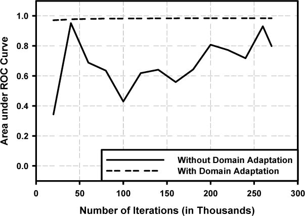
Performance of deep convolutional neural network (DCNN) on the validation set. The area under the ROC (AUC) was used as the figure of merit for model selection. Solid line: regular resampling; Dash line: domain adaptation resampling.

With the feature-based statistical learning approach, we used LASSO to generate the PMD. We varied the lambda in LASSO, which was the penalty term, to optimize the feature selection and PMD prediction. After optimization, lambda was chosen to be 9 × 10⁻⁵ for regular resampling and 4 × 10⁻⁵ for domain adaptation, which yielded maximum average validation AUCs of 0.960±0.004 and 0.962±0.003, respectively. The AUCs with domain adaptation was slightly better than that with regular resampling but the difference did not reach statistical significance. We used the domain adaptation results for comparison to DCNN results, as summarized in Table II.

Table II.

PD estimations by DCNN and statistical learning. The results for the cross validation testing used the domain adaptation resampling method. The results for the independent testing show the average from the model ensemble of 10 trained models.

	Cross Validation Test		Independent Test
	DCNN	Statistical Learning	DCNN	Statistical Learning
AUC	0.981±0.003	0.962±0.003	0.974±0.007	0.874±0.026
Dice Coefficient	0.79±0.13	0.72±0.18	0.78±0.08	0.63±0.22
Correlation	0.97	0.85	0.95	0.79
TP rate	0.90	0.88	0.88	0.69

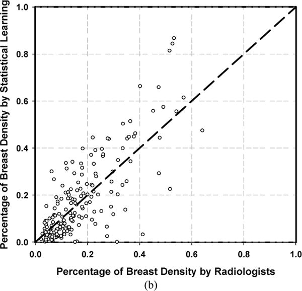
Figure 6 showed the scatter plots of PDs estimated by the DCNN and feature-based LASSO obtained with cross-validation compared to the reference standard from radiologists’ interactive thresholding. The Dice coefficients for the DCNN versus radiologist were 0.79±0.13 while that of LASSO versus radiologist was 0.72±0.18. The TP rate for the DCNN was 0.90 compared to 0.88 for LASSO. The correlation coefficient of DCNN was 0.97 while that of LASSO was 0.85. The two-tailed paired t-test between the differences in PDs from DCNN-vs-radiologist and those from statistical learning-vs-radiologist showed that the DCNN was significantly better than the statistical learning approach (p < 0.0001).

Figure 6.

Scatter plots of PDs estimated by the machine learning methods obtained with cross validation in model selection and evaluation versus radiologists’ interactive thresholding. (a) DCNN, (b) Feature-based statistical learning.

After the cross validation, we applied the developed models to the independent test set. For independent testing, we used two approaches: 1) retrained the models with the entire set of 478 DMs to maximize the training samples; and 2) applied the model ensemble, in which the 10 trained models from the 10-fold cross validation were applied to the test DMs and a mean PMD was obtained by averaging pixel by pixel of the 10 PMDs. For DCNN, the Dice coefficients versus radiologist were 0.76±0.09 and 0.78±0.08, the TP rates were 0.87 and 0.88, and the correlation coefficients with radiologist were 0.94 and 0.95 by using the retrained model and the model ensemble, respectively. For statistical learning, the Dice coefficients versus radiologist were 0.62±0.21 and 0.63±0.22, the TP rates were 0.71 and 0.69, while the correlation coefficients with radiologist were 0.75 and 0.79 by using the retrained model and the model ensemble, respectively. Figure 7 showed the scatter plot of PDs estimated by the DCNN and feature-based statistical learning obtained with independent testing compared to the reference standard when we used the model ensemble. Figure 8 showed the histograms of pixel-wise gray-level, LASSO score and DCNN score on fatty group and dense group for the independent test set.

Figure 7.

Scatter plots of PDs estimated by the machine learning methods obtained with independent testing of 183 DMs versus radiologists’ interactive thresholding. (a) DCNN, (b) Feature-based statistical learning.

Figure 8.

Histograms of pixel-wise gray-level (upper), LASSO score (middle), and DCNN score (lower) for the fatty class and dense class in the independent test set. The reference standard of fatty and dense is provided by radiologist.

IV. DISCUSSION

We developed a DCNN by supervised training for PD estimation. DCNN has the ability for automated image feature learning with convolutional layers. In our statistical learning method, we implemented features that were previously designed based on domain knowledge. We chose LASSO as the classifier to combine the features for the final prediction due to LASSO’s ability to perform feature selection and feature fusion in the same process. Compared with feature-based statistical learning method, the results demonstrated that our DCNN approach was significantly better and more robust in both validation and independent testing. The automated PD estimated by DCNN was highly correlated with the PDs by radiologists’ interactive thresholding. The small upward bias could be reduced by selecting a higher threshold on the PMD for separating the dense pixels from fatty pixels. The current threshold was chosen at the probability of 0.5 without specific learning from the samples.

Our approach in this study was to learn a pixel-wise PMD with a training set of digital mammograms. During the training, we used the 10-fold cross validation technique to select the model. Within each training iteration, a mini batch stochastic gradient descent (mSGD) method was used for parameter optimization through backpropagation. The output layer of our DCNN contained two competing neurons that represented the odds of the central pixel of the input image patch being fatty or dense. Compared to the regular gradient descent (rGD) method in which the model parameters are updated with the backpropagated errors after processing all of the samples, mSGD updates the model parameters after processing all samples in a mini batch. Although mSGD is much faster compared to rGD, the error function of mSGD is often not as well minimized as in the case of rGD. The challenge in training the DCNN for this task was that our training set was skewed to the fatty pixel class. The mini batch used for parameter optimization in each training iteration was randomly drawn from the training set. The characteristics of the samples in the training set would affect the DCNN training as illustrated in Figure 5. Our domain adaptation approach was designed to approximately balance the chances that dense and fatty pixels would be selected in each training mini batch while the total sample size was not reduced too much. Training with a more balanced mix of samples would reduce the chance that the trained DCNN might be skewed by the oversampling of one competing class. The threshold of 0.2 on the PD values was a hyperparameter empirically chosen for our training set due to the fact that 54.8% of images (262 out of 478 images) had a PD less than 0.2. By halving the number of images that had PD less than 0.2, we could potentially achieve more balanced mix of samples during DCNN training. The chosen threshold might need to be adjusted if the collected training set had a different distribution of fatty and dense breasts. From Figure 5, we observed that the training process with domain adaptation was much more stable than that without domain adaptation. This indicated that our domain adaptation is an important regularization step that can help the DCNN converge to a stable solution. Furthermore, the generalizability and outcomes of the trained DCNN depend on the stability of overall training process and, once trained, should not be affected by this hyperparameter. Depending on the training set and target task, one may find a stable solution with other regularization methods, such as layer normalization, maximum pooling, and adding L1/L2 terms during DCNN training. We have already incorporated layer normalization, maximum pooling, and L2 regularization terms into our DCNN structure. However, our experiments showed that the domain adaptation strategy still played an important role during DCNN training with the skewed training set.

In general, DCNN training requires a large number of manually annotated samples in order to avoid overfitting. In this study, we generated nearly 1 million image patches for DCNN training. Although the number of patches was huge, a lot of patches may be highly correlated because of the physical overlap as well as the fact that many patches were extracted from each image. Our domain adaptation resampling was designed to further regularize the DCNN training. It was found that domain adaptation resampling substantially improved the training stability of DCNN in our application. In contrast, its effect on statistical learning was not obvious although it was slightly better than regular cross validation. This may be due to the simplicity of LASSO in comparison to DCNN.

In this study, we chose our network structure based on previous studies (Pinto et al 2009, Cox and Pinto 2011). Our network structure was inspired by HT-L3 network (Pinto et al 2009). The HT-L3 convolutional network with 3 feature generation layers is a technique for learning feature representations of images through an architecture search procedure. They compared the results of HT-L2 and HT-L3, and observed that HT-L3 had a better performance. Fonseca et al. (Fonseca et al 2017) recently found that HT-L3 was a good feature extractor for automated BI-RADS density classification in which the convolutional layers were fixed with pre-trained weights using the ImageNet dataset.

Although the PD by DCNN was highly correlated with radiologist’s PD, there were outliers in both validation and independent testing. Figure 9 shows two image examples, in which the absolute differences between PDs of DCNN and radiologist were over 0.10. We observed that the breast with higher density (BI-RADS D) was relatively error-prone in comparison to radiologist’s PD. Two results may contribute to this observation: 1) our current preprocessing method did not enhance sufficient parenchymal features in dense breasts in comparison to its enhancement of relatively fatty breasts; and 2) our current data set did not provide enough samples of dense breasts for the DCNN training.

Figure 9.

Two image examples with inferior PD estimation by DCNN. From left to right: processed DMs, reference standard by radiologist, and the segmentation by DCNN.

As observed in many studies, the deeper of a DCNN structure the better its learning capacity. On the other hand, the deeper the DCNN, the bigger the training set it usually requires for robust training. The learning capacity required will depend on the complexity of a give pattern recognition task. Recently, transfer learning has been recognized as an important approach in deep learning application. Some well-designed deep learning structures, such as AlexNet (Krizhevsky et al 2012), GoogleNet (Szegedy et al 2015) and ResNet (He et al 2016) that have achieved good performance in natural scene images by training with millions of image samples, have been used for transfer learning in different pattern recognition tasks that have limited available samples such as medical images. We will explore transfer learning in our application in future work as well. Instead of transfer learning, unsupervised feature learning is another approach for the pre-training of deeper neural networks. Kallenberg et al. (Kallenberg et al 2016) used a sparse autoencoder to learn the multiscale features for mammographic density. Their approach achieved a correlation of 0.85-0.93 between the computer and a human reader, and a Dice coefficient of 0.63 in dense breast and 0.95 in fatty breast. They demonstrated the promise of unsupervised learning even when the network was not very deep in comparison to the above DCNNs.

There are limitations in this study. First, our data set was collected from mammography systems of a single vendor. Our method will need to be further validated using images from other mammography imaging systems. Second, we used the “for processing” DM as the input so that the trained DCNN will be more robust across different vendors’ imaging systems. However, some institutions may not save the “for processing” DMs. It remains to be studied whether our trained DCNN may be applicable to the “for presentation” images. Nevertheless, our proposed approach is general so that the DCNN may only require proper transfer learning or certain normalization of the input images in order to be translated to DMs from other vendors’ imaging systems or “for presentation” DMs. Third, in our domain adaptation, we reduced the proportion of fatty breasts to balance the overall distribution of dense and fatty breasts in the training population. Alternatively, we could over-sample the other group to balance the classes and evaluate the performances during training and validation. Either way would improve the balance of the classes in the training set, which was shown to provide more robust training. We will continue to collect additional case samples, especially those of dense breasts, for further finetuning of our DCNN.

V. CONCLUSION

We have developed a novel method based on deep learning for estimation of the percentage of breast dense area on DMs. Our DCNN method was trained to learn PMD in a two-class classification setting. We trained the DCNN using a patch-wise approach, which ensured sufficient number of training samples during the neural network optimization. Our automated tool by deep learning has potential applications for breast density reporting as well as for model-based risk prediction.

References

- American College of Radiology (ACR) Breast Imaging Reporting and Data System Atlas (BI-RADS® Atlas) No. American College of Radiology; 2013. [Google Scholar]
- Arefan D, Talebpour A, Ahmadinejhad N, Asl AK. Automatic breast density classification using neural network. Journal of Instrumentation. 2015;10:1–9. [Google Scholar]
- Berg WA, Campassi C, Langenberg P, Sexton MJ. Breast Imaging Reporting and Data System: Inter- and Intraobserver variablity in feature analysis and final assessment. American Journal of Roentgenology. 2000;174:1769–77. doi: 10.2214/ajr.174.6.1741769. [DOI] [PubMed] [Google Scholar]
- Boyd N, Byng J, Jong R, Fishell E, Little L, Miller A, Lockwood G, Tritchler D, Yaffe M. Quantitative classification of mammographic densities and breast cancer risk: results from the Canadian National Breast Screening Study. Journal of the National Cancer Institute. 1995;87:670–5. doi: 10.1093/jnci/87.9.670. [DOI] [PubMed] [Google Scholar]
- Boyd NF, Guo H, Martin LJ, Sun L, Stone J, Fishell E, Jong RA, Hislop G, Chiarelli A, Minkin S, Yaffe MJ. Mammographic Density and the Risk and Detection of Breast Cancer. New England Journal of Medicine. 2007;356:227–36. doi: 10.1056/NEJMoa062790. [DOI] [PubMed] [Google Scholar]
- Brandt KR, Scott CG, Ma L, Mahmoudzadeh AP, Jensen MR, Whaley DH, Wu FF, Malkov S, Hruska CB, Norman AD, Heine J, Shepherd J, Pankratz VS, Kerlikowske K, Vachon CM. Comparison of Clinical and Automated Breast Density Measurements: Implications for Risk Prediction and Supplemental Screening. Radiology. 2015;279:710–9. doi: 10.1148/radiol.2015151261. [DOI] [PMC free article] [PubMed] [Google Scholar]
- Burt PJ, Adelson EH. The Laplacian Pyramid as a Compact Image Code. IEEE Transactions on Communications. 1983;31:532–40. [Google Scholar]
- Byng JW, Boyd NF, Fishell E, Jong RA, Yaffe MJ. The quantitative-analysis of mammographic densities. Phys Med Biol. 1994;39:1629–38. doi: 10.1088/0031-9155/39/10/008. [DOI] [PubMed] [Google Scholar]
- Chan H-P, Lo S-CB, Helvie MA, Goodsitt MM, Cheng S, Adler DD. Recognition of mammographic microcalcifications with artificial neural network. RSNA Program Book. 1993;189(P):318. [Google Scholar]
- Chan H-P, Lo S-C B, Sahiner B, Helvie MA. Computer-aided detection of mammographic microcalcifications: pattern recognition with an artificial neural network. Medical Physics. 1995;22:1555–67. doi: 10.1118/1.597428. [DOI] [PubMed] [Google Scholar]
- Cox D, Pinto N. Beyond simple features: A large-scale feature search approach to unconstrained face recognition. Face and Gesture. 2011 2011 8-15 21-25 March 2011. [Google Scholar]
- Dice LR. Measures of the amount of ecologic association between species. Ecology. 1945;26:297–302. [Google Scholar]
- Engmann NJ, Golmakani MK, Miglioretti DL, Sprague BL, Kerlikowske K, for the Breast Cancer Surveillance C Population-attributable risk proportion of clinical risk factors for breast cancer. JAMA Oncology. 2017 doi: 10.1001/jamaoncol.2016.6326. [DOI] [PMC free article] [PubMed] [Google Scholar]
- Fonseca P, Castaneda B, Valenzuela R, Wainer J. CIARP 2016. LNCS 10125. Springer; 2017. Breast density classification with convolutional neural networks; pp. 101–8. [Google Scholar]
- Goodfellow I, Bengio Y, Courville A. Deep Learning. The MIT Press; 2016. [Google Scholar]
- Hastie T, Tibshirani R, Friedman J. The elements of statistical learning: data mining, inference, and prediction (second edition) Springer; 2011. [Google Scholar]
- He K, Zhang X, Ren S, Sun J. Deep residual learning for image recognition; IEEE Conference on Computer Vision and Pattern Recognition (CVPR); 2016. pp. 770–8. [Google Scholar]
- Highnam R, Brady MJ. Mammographic image analysis. Dordrecht: Kluwer Academic Publishers; 1999. [Google Scholar]
- Highnam R, Pan X, Warren R, Jeffreys M, Smith GD, Brady M. Breast composition measurements using retrospective standard mammogram form (SMF) Physics in Medicine and Biology. 2006;51:2695. doi: 10.1088/0031-9155/51/11/001. [DOI] [PubMed] [Google Scholar]
- Hinton GE, Srivastava N, Krizhevsky A, Sutskever I, Salakhutdinov RR. Improving neural networks by preventing co-adaptation of feature detectors. 2012 arXiv: 1207. 0580 [cs.NE] [Google Scholar]
- Hubel DH, Wiesel TN. Receptive fields of single neurones in the cat’s striate cortex. The Journal of Physiology. 1959;148:574–91. doi: 10.1113/jphysiol.1959.sp006308. [DOI] [PMC free article] [PubMed] [Google Scholar]
- Kallenberg M, Petersen K, Nielsen M, Ng AY, Diao P, Igel C, Vachon CM, Holland K, Winkel RR, Karssemeijer N, Lillholm M. Unsupervised Deep Learning Applied to Breast Density Segmentation and Mammographic Risk Scoring. IEEE Transactions on Medical Imaging. 2016;35:1322–31. doi: 10.1109/TMI.2016.2532122. [DOI] [PubMed] [Google Scholar]
- Keller BM, Nathan DL, Wang Y, Zheng Y, Gee JC, Conant EF, Kontos D. Estimation of breast percent density in raw and processed full field digital mammography images via adaptive fuzzy c-means clustering and support vector machine segmentation. Medical Physics. 2012;39:4903–17. doi: 10.1118/1.4736530. [DOI] [PMC free article] [PubMed] [Google Scholar]
- Kerlikowske K. The Mammogram That Cried Wolfe. New England Journal of Medicine. 2007;356:297–300. doi: 10.1056/NEJMe068244. [DOI] [PubMed] [Google Scholar]
- Krizhevsky A, Sutskever I, Hinton GE. ImageNet Classification with Deep Convolutional Neural Networks Neural Information Processing Systems (NIPS) 2012:1097–105. [Google Scholar]
- Lauby-Secretan B, Scoccianti C, Loomis D, Benbrahim-Tallaa L, Bouvard V, Bianchini F, Straif K. Breast-Cancer Screening — Viewpoint of the IARC Working Group. New England Journal of Medicine. 2015;372:2353–8. doi: 10.1056/NEJMsr1504363. [DOI] [PubMed] [Google Scholar]
- Litjens GJS, Kooi T, Bejnordi BE, Setio AAA, Ciompi F, Ghafoorian M, van der Laak J, van Ginneken B, Sánchez CI. A Survey on Deep Learning in Medical Image Analysis. Medical Image Analysis. 2017;42:60–88. doi: 10.1016/j.media.2017.07.005. [DOI] [PubMed] [Google Scholar]
- Lo S-CB, Chan H-P, Lin J-S, Li H, Freedman MT, Mun SK. Artificial convolution neural network for medical image pattern recognition. Neural Netw. 1995a;8:1201–14. [Google Scholar]
- Lo S-CB, Lou S-LA, Lin J-S, Freedman MT, Chien MV. Artificial convolution neural network techniques and applications for lung nodule detection. IEEE Transactions on Medical Imaging. 1995b;14:711–8. doi: 10.1109/42.476112. [DOI] [PubMed] [Google Scholar]
- Lo SC, Lin JS, Freedman MT, Mun SK. Computer-assisted diagnosis of lung nodule detection using artificial convolution neural network. Proc SPIE. 1993;1898:859–69. [Google Scholar]
- Martin KE, Helvie MA, Zhou C, Roubidoux MA, Bailey JE, Paramagul C, Blane CE, Klein KA, Sonnad SS, Chan H-P. Mammographic Density Measured with Quantitative Computer-aided Method: Comparison with Radiologists’ Estimates and BI-RADS Categories. Radiology. 2006;240:656–65. doi: 10.1148/radiol.2402041947. [DOI] [PubMed] [Google Scholar]
- McCormack VA, dos Santos Silva I. Breast Density and Parenchymal Patterns as Markers of Breast Cancer Risk: A Meta-analysis. Cancer Epidemiology Biomarkers & Prevention. 2006;15:1159–69. doi: 10.1158/1055-9965.EPI-06-0034. [DOI] [PubMed] [Google Scholar]
- Nair V, Hinton GE. Rectified linear units improve restricted boltzmann machines; Proceedings of the 27th international conference on machine learning (ICML-10); 2010. pp. 807–14. [Google Scholar]
- Oliver A, Tortajada M, Lladó X, Freixenet J, Ganau S, Tortajada L, Vilagran M, Sentís M, Martí R. Breast Density Analysis Using an Automatic Density Segmentation Algorithm. Journal of Digital Imaging. 2015;28:604–12. doi: 10.1007/s10278-015-9777-5. [DOI] [PMC free article] [PubMed] [Google Scholar]
- Otsu N. A threshold selection method from gray-level histograms. IEEE Trans Syst Man Cybern. 1979;9:62–6. [Google Scholar]
- Pinto N, Doukhan D, DiCarlo JJ, Cox DD. A High-Throughput Screening Approach to Discovering Good Forms of Biologically Inspired Visual Representation. PLOS Computational Biology. 2009;5:e1000579. doi: 10.1371/journal.pcbi.1000579. [DOI] [PMC free article] [PubMed] [Google Scholar]
- Saftlas A, Hoover R, Brinton L, Szklo M, Olson D, Salane M, Wolfe J. Mammographic densities and risk of breast cancer. Cancer. 1991;67:2833–88. doi: 10.1002/1097-0142(19910601)67:11<2833::aid-cncr2820671121>3.0.co;2-u. [DOI] [PubMed] [Google Scholar]
- Sahiner B, Chan H-P, Petrick N, Wei D, Helvie MA, Adler DD, Goodsitt MM. Classification of mass and normal breast tissue: A convolution neural network classifier with spatial domain and texture images. IEEE Transactions on Medical Imaging. 1996;15:598–610. doi: 10.1109/42.538937. [DOI] [PubMed] [Google Scholar]
- Siegel RL, Miller KD, Jemal A. Cancer statistics, 2017. CA: A Cancer Journal for Clinicians. 2017;67:7–30. doi: 10.3322/caac.21387. [DOI] [PubMed] [Google Scholar]
- Szegedy C, Ioffe S, Vanhoucke V, Alemi AA. Inception-v4, inception-resnet and the impact of residual connections on learning; 4th International Conference on Learning Representations (ICLR); San Juan. 2016. arXiv:1602.07261. http://www.iclr.cc/doku.php?id=iclr2016:main. [Google Scholar]
- Szegedy C, Wei L, Yangqing J, Sermanet P, Reed S, Anguelov D, Erhan D, Vanhoucke V, Rabinovich A. Going deeper with convolutions; InIEEE Conference on Computer Vision and Pattern Recognition (CVPR); 2015. pp. 1–9. [Google Scholar]
- Tice JA, Cummings SR, Ziv E, Kerlikowske K. Mammographic Breast Density and the Gail Model for Breast Cancer Risk Prediction in a Screening Population. Breast Cancer Research and Treatment. 2005;94:115–22. doi: 10.1007/s10549-005-5152-4. [DOI] [PubMed] [Google Scholar]
- Vachon CM, Brandt KR, Ghosh K, Scott CG, Maloney SD, Carston MJ, Pankratz VS, Sellers TA. Mammographic Breast Density as a General Marker of Breast Cancer Risk. Cancer Epidemiology Biomarkers & Prevention. 2007;16:43–9. doi: 10.1158/1055-9965.EPI-06-0738. [DOI] [PubMed] [Google Scholar]
- Wei J, Chan H-P, Helvie MA, Roubidoux MA, Sahiner B, Hadjiiski L, Zhou C, Paquerault S, Chenevert T, Goodsitt MM. Correlation between mammographic density and volumetric fibroglandular tissue estimated on breast MR images. Medical Physics. 2004;31:933–42. doi: 10.1118/1.1668512. [DOI] [PubMed] [Google Scholar]
- Wei J, Sahiner B, Hadjiiski LM, Chan HP, Petrick N, Helvie MA, Roubidoux MA, Ge J, Zhou C. Computer aided detection of breast masses on full field digital mammograms. Medical Physics. 2005;32:282738. doi: 10.1118/1.1997327. [DOI] [PMC free article] [PubMed] [Google Scholar]
- Wolfe JN. Breast patterns as an index of risk for developing breast cancer. American Journal of Roentgenology. 1976;126:1130–7. doi: 10.2214/ajr.126.6.1130. [DOI] [PubMed] [Google Scholar]
- Wolfe JN, Saftlas AF, Salane M. Mammographic parenchymal patterns and quantitative evaluation of mammographic densities: a case-control study. American Journal of Roentgenol. 1987;148:108792. doi: 10.2214/ajr.148.6.1087. [DOI] [PubMed] [Google Scholar]
- Zhou C, Chan H-P, Petrick N, Helvie MA, Goodsitt MM, Sahiner B, Hadjiiski LM. Computerized image analysis: Estimation of breast density on mammograms. Medical Physics. 2001;28:1056–69. doi: 10.1118/1.1376640. [DOI] [PubMed] [Google Scholar]
- Zoe Aitken VAM, Highnam Ralph P, Martin Lisa, Gunasekara Anoma, Melnichouk Olga, Mawdsley Gord, Peressotti Chris, Yaffe Martin, Boyd Norman F, dos Santos Silva Isabel. Screen-Film Mammographic Density and Breast Cancer Risk: A Comparison of the Volumetric Standard Mammogram Form and the Interactive Threshold Measurement Methods. Cancer Epidemiology, Biomarkers & Prevention. 2010;19:418–28. doi: 10.1158/1055-9965.EPI-09-1059. [DOI] [PMC free article] [PubMed] [Google Scholar]