Abstract
In this work, we consider the problem of estimating multiple sparse, co-activated brain regions from functional magnetic resonance imaging (fMRI) observations belonging to different classes. More precisely, we propose a method to analyze similarities and differences in functional connectivity between children and young adults. Often, analysis is conducted on each class separately, and differences across classes are identified with an additional postprocessing step using various statistical tools. Here, we propose to rely on a generalized fused Lasso penalty, which allows us to make use of the entire dataset in order to estimate connectivity patterns that are either shared across classes, or specific to a given group. By using the entire population during the estimation, we hope to increase the power of our analysis. The proposed model falls in the category of population-wise matrix decomposition, and a simple and efficient alternating direction method of multipliers (ADMM) algorithm is introduced to solve the associated optimization problem. After validating our approach on simulated data, experiments are performed on resting-state fMRI imaging from the Philadelphia Neurodevelopmental Cohort (PNC) dataset, comprised of normally developing children from ages 8 to 21. Developmental differences were observed in various brain regions, as a total of 3 class-specific resting-state components were identified. Statistical analysis of the estimated subject-specific features, as well as classification results (based on age groups, up to 81% accuracy, n = 583 samples) related to these components demonstrate that the proposed method is able to properly extract meaningful shared and class-specific sub-networks.
Index Terms: Sparse Models, Joint Lasso Penalty, Functional Connectivity, Brain Development
I. Introduction
Neuroimaging data is heavily used to analyze both brain functions and brain structure. In particular, functional magnetic resonance imaging (fMRI) provides non-invasive measurements over a time frame of seconds with a spatial resolution of millimeters. Many fMRI analyses are interested in functional segregation (i.e. the identification of specialized brain areas for a given task) as well as functional integration (i.e. coordinated cerebral activity between brain regions)[1]. In this paper, we will be interested in the latter. More precisely, we will rely on functional connectivity measures for the discovery of statistical patterns of cerebral activity across various brain regions.
A significant number of studies have been conducted to gain insight about the changes in brain functional activity that occur throughout childhood and adolescence[2], [3]. Although the functional organization of the human brain in childhood is not very well understood yet, it appears that the basic configuration of functional activity networks are established around the age of 12[3]. Indeed, several developmental fMRI studies showed that core regions of functional networks can be observed already in early development [4], [5]. We may then expect, to a certain extent, to extract ‘similar’ overall profiles of connectivity patterns between children and young adults. This will be of particular interest later in the paper to justify the use of a Fused Lasso penalty in the proposed model.
A common assumption is that the brain operates as a set of distributed sub-networks[6] that co-activate over time. As a consequence, there is a great interest in correctly identifying these sub-networks using, among others, fMRI data. For example, the analysis of resting state fMRI sequences (i.e., in the absence of an explicit experimental task to be performed by the subject) enables one to extract spontaneous patterns/sub-networks of neuronal activity arising when a person is at rest. Many such common patterns or co-activated networks including, e.g., the default mode network (DMN) or the sensory motor network, are now well known and are reliably identified by the research community[7], [8]. In this work, the emphasis will be put on the identification and analysis of discriminative connectivity patterns across different classes. There are many ways to extract meaningful connectivity information from fMRI blood-oxygenation-level dependent (BOLD) time series, and a compelling framework is to represent the brain as a network:
Nodes are often defined from a given list of regions of interest (ROI, based on brain atlases[9], [10]), data-driven components (e.g. using independent component analysis (ICA)[11]) or even down to single voxels;
Edges are often characterized by statistical dependencies between pairs of nodes (or, more generally, groups of nodes). There are several ways to measure functional connectivity: coherence measure, Pearson correlation, mutual information or partial correlation. In this work, we rely on Pearson correlation in order to measure functional connectivity.
Various computational approaches have been proposed for the identification of functional sub-networks. One of the most commonly used method is seed-based correlation analysis (SBA)[12]. Starting from a user-specified seed region/voxel, successive hypotheses of statistical relationship with other target regions/voxels are tested to derive a brainwide connectivity map with respect to the seed. A number of methods have also utilized graph-based frameworks[13], [14]. Independent component analysis (ICA) is an interesting data-driven tool that has been applied[15] to identify maximally independent spatial/temporal maps from BOLD time series. Non-negative matrix factorization (NMF) methods[16], [17] are increasingly used to extract multiple potentially overlapping brain networks by decomposing data matrices into linear combinations of non-negative basis functions. Other matrix decompositions methods such as Principal Component Analysis (PCA)[18] have been to used to extract intrinsic structure in the data by maximizing the amount of variance explained. More recently, Eavani et al.[6] defined quantities referred to as sparse connectivity patterns (SCP), as well as a complete framework for their estimation. Extracted from subjects’ pairwise correlation matrices, these SCPs are essentially sparse, spatially distributed and synchronous sub-networks that aim to represent different co-activated functional brain regions. We provide further details about their formulation and estimation in the next section. Interestingly, similar to the discriminative dictionary learning methods used in computer vision (for example, see Yang et al.[19]), the same authors proposed an SCP estimation model with a discriminative flavor earlier in [20]. However, in both works, they only extract one global set of SCP for the entire population. In this work, we extend such formulation to work with data belonging to different groups/classes. This allows us to naturally extract class-specific sets of SCP. Furthermore, as we previously stated, it is reasonable to expect a certain degree of similarities across children and young adults in terms of global functional network structures. We then propose to use a generalized fused Lasso penalty to estimate these sets of SCP by jointly using data from both classes. As we will show later in this paper, this leads to an increased estimation power in terms of SCP components that are common between children and young adults. As a consequence, and maybe more importantly, it is of great help to identify class-specific patterns within these SCP as well.
The rest of this paper is organized as follows: we present in Section 2 the concept of SCP introduced by Eavani et al.[6] and propose an extended ‘fused’ formulation in the case of multi-class setups. Our new method is then evaluated on both synthetic data and real data (PNC[21]) in Section 3, followed by some discussions and concluding remarks in Section 4.
II. Identifying shared and differential networks
A. Presentation of the model
We start by formulating the problem of SCP identification as defined by Eavani et. al[6]. Let us assume we have n ∈ ℕ subjects. For each subject, a BOLD time series of nt time points and p ROI (nt, p ∈ ℕ) is available. Denote Ci ∈ ℝp×p, i = 1, .., n, the association matrix for each subject; Ci(p1, p2) is simply in our case the Pearson correlation value between ROI p1 and p2 along the entire BOLD time series. We can estimate d ∈ ℕ (d ≤ p) SCP by solving the following problem:
| (1) |
where λ1 is a non-negative model parameter, ‖·‖F denotes the Frobenius norm, x = [x1, .., xd] ∈ ℝp×d, Wi ∈ ℝd×d is a diagonal matrix ∀i = 1, .., n, and W = {W1, .., Wn}. Notation Wi ⪰ 0 means that elements of each matrix Wi are assumed to be positive, and a constraint on each SCP xj using infinity norm is added to avoid any scaling ambiguity[6]. Eq. 1 can be reframed as a sparse population-level rank-d approximation of the set of correlation matrices:
Each of the d columns of x define a SCP, i.e. a set of co-activated regions;
Positive coefficients from each diagonal matrix Wi provide ‘subject-specific’ maps expressing how much a given SCP is expressed in the i-th subject’s correlation matrix Ci.
Note that the two ROIs p1, p2 are considered to be strongly co-activated within a given SCP if for the corresponding column of x, both the p1-th and p2-th coefficients are non zero. Similarly, if the p1-th and p2-th coefficients are non zeros and of opposite sign, ROI p1, p2 will be considered anti-activated. Essentially, such approach reduces the high dimensionality of the set of correlation matrices by extracting a small subset of strongly correlated (and anti-correlated) components. Subject specific weight maps locally measure how much each SCP is expressed in each subject.
Let us now assume our observations can be divided into K distinct classes. This can be represented with a label value yi ∈ ℤ, i = 1, .., n, for each subject. A direct ‘supervised-flavored’ extension of Eq. 1 would be to solve the following problem:
| (2) |
where is the set of observations belonging to the k-th class (k = 1, .., K), and xk ∈ ℝp×d is the SCP for the k-th class. Note that both constraints on the weight matrices and the SCP scaling from Eq. 1 have been omitted for the sake of simplicity. Let us stress the fact that the model from Eq. 2 essentially amounts to performing a separate analysis on populations from different classes. As a consequence, no information is shared across the different classes while performing the SCP estimation. In practice, one would expect the set of SCPs xk, k = 1..K to share a certain degree of similarity among the different classes. By performing separate analyses, we can not exploit these similarities. Conversely, estimating a global model for all classes might overlook some important distinctions between the classes, and make it impossible to extract discriminative patterns across these classes. Inspired by the work of Danaher et al.[22], we propose to further regularize model from Eq. 2 in order to take into account shared patterns among classes. This new model takes the following form:
| (3) |
where λ2 is a non-negative model parameter, and xk,j denotes the j-th SCP (i.e. column of xk) of the k-th class. We can see that this new regularization term essentially amounts to applying the ℓ1 penalty between corresponding elements of each pair of SCP across classes. As a result, for increasing values of λ2, more and more components of x1, .., xK will be identical: it encourages different classes to share SCP components. Such penalty has been successfully applied before to joint Gaussian graphical model estimation[22] as well as cross-correlation analysis formulation for extracting imaging genomic modules, as in our recent work [23]. A schematic diagram illustrating our approach can be seen in Figure 1. In the next section, we provide some details on how to solve Eq. 3, specifically in the case where K = 2.
Fig. 1.
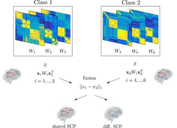
Simplified illustration of the proposed method in the case of two classes. Using correlation matrices from each class, we extract sets of co-activated sub-networks (Sparse Connectivity Patterns, or SCP) represented by the components of vectors xk, k = 1, 2. In this simple case, a single SCP (i.e. column vector) is estimated for each class. These SCP’s are fused across classes during estimation depending on the weight parameter λ2 in Eq. 3. This allows us to extract SCP components that are shared across classes (red sub-network) with an increased analysis power, since the whole dataset is used. This in turns facilitates further identification of differential/class-specific SCP (green and blue sub-networks).
B. Optimization
In order to optimize the model defined in Eq. (3), we rely on the alternating direction method of multipliers[24] (ADMM). Based on variable splitting, it provides a generic and powerful framework to solve a wide variety of problems. Let us consider the following problem:
| (4) |
By setting and , we essentially fall back into a split version of Eq. (3). It can be shown[24] that solving Eq. (4) can be done by breaking down the original optimization into several subproblems that are often much easier to solve separately. The general form of the minimization algorithm can be seen in Algorithm 1.
In practice, we do not try to solve model from Eq. 3 directly. Instead, we adopt a sequential approach and estimate each SCP one after another. This greatly simplifies the overall estimation process and algorithm development. Suppose we already have at hand a set of r ∈ ℕ estimated SCP , as well as their associated subject-specific weight maps , i = 1, .., n. For each correlation matrix Ci, i = 1, .., n, we can compute a new deflated matrix such that
and perform the estimation of an additional SCP xr+1 by using the deflated matrices , i = 1, .., n. Comparison between such sequential approach and Eavani’s original one can be found in supplementary material (Appendix A). The overall procedure is described in Alg 2. The ADMM algorithm described in Alg. 1 is essentially iterative in nature. As a consequence, convergence might turn out to be slow in some cases. Fortunately, an efficient initialization of x0 that proved to work well during our experiments can be obtained at fairly low cost: one just needs to perform a rank-d approximation of each , i.e. the mean correlation matrix for each class. Looking for the solution from this starting point facilitates greatly the overall estimation compared to, for example, a random initialization. In our case, solving the x-update of Algorithm 1, line 4, with a few gradient estimations has proven to work well during our tests. Regarding the z-update of line 5, an efficient method in the case of K = 2 classes is detailed in [22]. In such case, a closed form solution for the minimum can be obtained in two steps. First, we calculate:
where the above operations have to be taken component wise, although the component index is omitted for the sake of simplicity. Finally, we just need to apply a soft-thresholding[25] operator with a factor of λ1/ρ to the resulting ( , ). In the case where more than two classes are present, more advanced and computationally expansive methods have to be used. In this work, we will restrict ourselves to only 2 classes, and refer the reader to [22] for further details.
Algorithm 1.
General ADMM minimization algorithm
| 1: | Initialize x0, z0, u0 ∈ ℝp |
| 2: | Input regularization parameter ρ ∈ ℝ |
| 3: | for k = 0 to Convergence do |
| 4: | |
| 5: | |
| 6: | |
| 7: | end for |
Algorithm 2.
Joint SCP estimation algorithm
| 1: | Compute correlation matrices Ci, i = 1..n |
| 2: | Input parameters λ1, λ2, d. |
| 3: | for r = 1 to d do |
| 4: | if r ≥ 1 then |
| 5: | Deflate input correlation matrices using previous estimation . |
| 6: | else |
| 7: | |
| 8: | end if |
| 9: | Estimate xr using and ADMM algorithm from Alg. 1. |
| 10: | Normalize xr such that maxi |xr(i)| = 1. |
| 11: | end for |
C. Tuning parameter selection
One of the key aspects of the sparse estimation models defined in Eq. 1 or Eq. 3 is to find satisfactory regularization parameters values. The proposed fused SCP estimation model described in Eq. 3 requires the estimation of 3 key parameters: the number of SCP’s to be estimated d, the sparsity constraint’s weight λ1 and the fused constraint’s weight λ2. In their original paper, Eavani et al.[6] relied on a reconstruction error measure (first term from Eq. 1) within a training/test set up. On limitation of such approach is that the reconstruction error monotonically decreases with an increasing the value of d. As a consequence, they retained the value of d for which a ‘knee’ in the error plot could be observed. This led them to estimate d = 10 SCPs.
As our model is essentially a multi-class one, we propose to rely in this work on classification error to chose the prarameters’ values. While the detailed process will be presented in the next section, we provide a brief outline of the criterion used in practice. Once class-specific/differential SCP have been estimated, we can compute subject specific representation coefficients that measure how much each differential SCP is expressed for each subject. These coefficients are then used as features within a classification step. To find the optimal parameters, we simply perform a nested gridsearch combined with a 10-fold cross validation using a standard support vector machine (SVM, see [26]). As it will be shown later in this work, relying on the classification error associated to the differential SCP’s coefficients provides a number of benefits compared to the original approach used in Eavani et al.[6]. Additional results regarding the influence of parameters λ1, λ2 over the solution can be found in supplementary material (Appendix B).
D. Fused estimation of differential SCP
In their previous work, Eavani et al.[6] provided an extensive analysis of the estimated SCP’s in a population of young adults. As a consequence, we chose to focus in this work on the analysis of the differential (or class-specific) components of the estimated SCP’s. In this section, we provide some details regarding the actual estimation of the differential components from the estimated SCP’s.
As mentioned before, we can compute a correlation matrix for each subject based on the pre-processed region-averaged time series. We can then apply the model described in Eq. (3) to these correlation matrices and estimate a set of SCP’s for each class (K = 2 here). Shared components are then defined as the pairs (i, j) ∈ [1, .., p]×[1, .., d] such that , where ε = 0.1. Differential/class-specific components , k = 1, .., 2 will then simply be defined as the pairs (i, j) ∈ [1, .., p]×[1, .., d] such that . As mentioned earlier, in order to estimate the key parameters (λ1, λ2, d), we carry out this fused SCP estimation process over 10 runs where each time, the original dataset is divided into training and test subsets (90% training, 10% test). For each of these runs, the model is fitted on the training data only. Once this is done and the shared components have been computed, the ‘contribution’ of is removed from both test and training data. For each correlation matrix Ci, i = 1, .., n, we compute a new deflated matrix such that
where is a diagonal matrix solution of
For each of these deflated matrices, we can then compute a weight vector relative to each differential scp such that . This leaves us, for each subject in the training and test set, with K = 2 sets of weight vectors in ℝd, measuring how much of the subject’s deflated matrix can be explained by each class’s differential component. We can then use these data in two ways:
Concatenate both for each patient, and use the resulting vector as a feature that we can input into a standard SVM classifier. We can then assess whether or not the estimated differential SCPs are truly discriminative across classes. As mentioned before, we also rely on such classification score in order to estimate the parameters (λ1, λ2, d);
We may also look at the distribution of these weights between classes on the test set. We will then be looking for noticeable population-wide discrepancies between young adults and children in terms of how are the differential SCP expressed in each class.
III. Results
In this section, we evaluate the proposed fused model from Eq. 3. Its performances will be assessed in terms of feature selection relevance, classification accuracy as well as statistical analysis of the resulting weight maps Wi.
A. Analysis on simulated dataset
1) Data generation pipeline
In order to validate our pro-posed fused approach, we used the SimTB toolbox1 (cf. Erhardt at al. [27]) to simulate BOLD time series. An illustrative view of the simulated data for one run can be seen in Fig. 2. This simulated dataset has n = 50 subjects divided in two classes, each class being made of 25 subjects. For each subject, we generate time series for p = 20 ROI, made of 120 time points and a TR value of 2 seconds. A total of d = 4 SCP’s are generated, whose sizes vary randomly between 3 to 6 nodes. An overlap between SCP’s is also randomly assigned between 0 and 2 nodes. A sample set of SCP’s map is displayed in Fig. 2(i). On top of that, we introduce two additional layers of variability across subjects in the following way:
For each subject, each SCP is assigned an active/inactive weight in a binary fashion. As a consequence, some SCP’s might be inactive for a given subject. For each simulated run, a population-wise activation map is defined, indicating, for each subject, which SCP is active or not. During our test, we randomly set 5 – 10% of all tuples (subject, SCP) to inactive. An example of such activation map can be seen in Fig. 2(ii). Let us stress the fact that if a SCP is inactive for a given subject, then correlation values between nodes of that SCP will be zero for this particular subject.
The data is simulated such that the last 3 SCP’s are common to both classes, while the first one is only active in the first class (i.e., the first SCP is a differential or class-specific SCP). That is, weights corresponding to the first SCP are set to zero for each subject belonging to the second class, as seen in the first row of Fig. 2(ii).
Fig. 2.
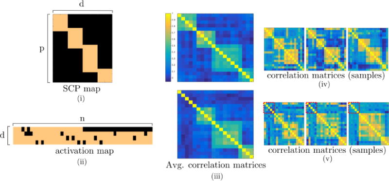
An illustrative view of one of the simulated datasets generated using SimTB toolbox. (i) SCP map for a given run. (ii) Population-wise activation map representing heterogeneity across subjects. Looking at the first row, notice that SCP 1 is assigned a weight of zero for the second class (second half of the subjects). (iii) Subject-average correlation matrices for first (top) and second (bottom) classes. (iv–v) Randomly selected subject’s correlation matrices. Dashed red squares indicate pairwise correlation between nodes belonging to the first SCP, i.e. the one consistently missing in the second class.
Subject-wise correlation matrices computed from the simulated BOLD series can be seen in Fig. 2(iv–v) for 6 randomly selected subjects (3 in each class), while subject averaged correlation matrices for each class are shown in Fig. 2(iii).
2) Results on simulated datasets
A common way to assess the performance of a model when it comes to feature extraction is to measure the true positive rate (TPR) and false positive rate (FPR). TPR reflects the proportion of variables (i.e. SCP components) that are correctly identified as non-zeros, while FDR reflects the proportion of variables that are incorrectly selected by the model as significant. Results can be displayed using a receiver operating characteristic (ROC) curve, illustrating the feature selection performances as the discrimination (selected/not-selected) threshold is varied. More succinctly, we plot the true positive rate (TPR) against the false positive rate (FPR). Such plots, averaged over 100 runs, can be seen for various values of λ1 and λ2 in Fig. 3. More precisely, two ROC curves can be computed: one for the components that are shared across classes, and one for the class specific components (i.e. associated to the first SCP). Taking a look at Fig. 3(a),(b), we can see that for different levels of sparsity (i.e., weight λ1 value), our proposed joint formulation leads to a better estimation of the shared component compared to the simple multi-class version of the model proposed by Eavani et. al (see Eq. 2, corresponding to model from Eq. 3 with λ2 = 0, i.e., no fusion effect). We can observe in Fig. 3(d),(e) the ROC curves on the class-specific components. When no sparsity constraint is enforced (i.e., λ1 = 0 in Fig. 3(d)), the results are fairly poor, and adding a fused penalty seems to lead to no improvement whatsoever, or even worsens the results. On the other hand, when sparsity is enforced (i.e., λ1 = 0.5 in Fig. 3(e)), we can see an generally improved estimation of the class-specific components. More interestingly, in this case, enforcing the fused penalty lead to an increased estimation power, achieving the overall best reconstruction of the class-specific components. Of course, if the fused weight parameter λ2 is set too high, the algorithm finds identical solutions across classes and no class-specific components can be estimated. If we pay attention to Fig. 3(c),(f) we can observe the evolution of the area under the ROC curve (AUC) as a function of λ2, for various λ1 values. Similar conclusions can be drawn: a non-zero value of λ2 greatly improves the estimation of the shared components. Interestingly, by looking at Fig. 3(f), we can observe that adding a fusion constraint can also improve the identification of the class-specific components, at least up to a certain point where the method just estimates identical SCP’s for each class (hence failing to retain class-specific components). In our opinion, these results are an illustration of the benefit of using a mix of sparsity and across-class fused constraints.
Fig. 3.
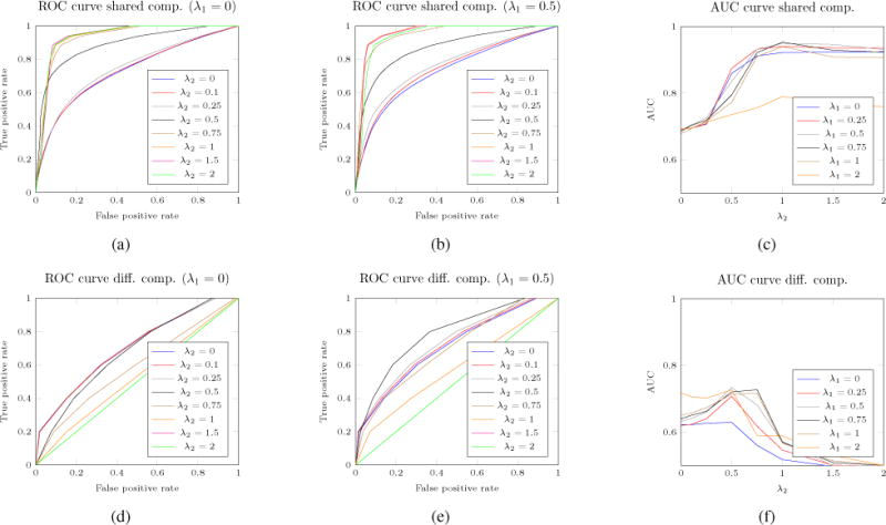
(a–b) The ROC curves for shared components for various sparsity levels (λ1 = {0, 0.5}). (d–e) ROC curves for differential/class-specific components for various sparsity levels (λ1 = {0, 0.5}).
B. Analysis of resting-state connectivity data
1) Data acquisition and preprocessing
The Philadelphia Neurodevelopmental Cohort[21] (PNC) is a large-scale collaborative study between the Brain Behaviour Laboratory at the University of Pennsylvania and the Children’s Hospital of Philadelphia. The data are available in the dbGaP database, which contains (among other data modalities[28]) rest fMRI data for nearly 900 adolescents age 8 to 21 years. Standard preprocessing steps were applied using SPM122, including motion correction, spatial normalization to standard MNI space (adult template) and spatial smoothing with an 3mm FWHM Gaussian kernel. The influence of motion (6 parameters) was further addressed using a regression procedure, and the functional time series were band-pass filtered using a 0.01Hz to 0.1Hz frequency range. Finally, we reduced the dimension of the data by using the 264 ROI atlas as defined by Power et al.[9] with a sphere radius parameter of 5mm. Since we are interested in brain development as a function of age, we select a subset of the full dataset based on age in months. More precisely, each subject whose age is over 200 months will belong to the first class (young adults cohort, age 18.72 ± 1.23 years, 157 females out of 290 subjects), while each subject whose age is under 160 months will belong to the second class (young cohort, age 11.13 ± 1.36 years, 148 females out of 293 subjects) .
2) Results on resting-state fMRI data
In this section, we display the estimated differential SCP as well as how differently they might be expressed across the two classes. Results are averaged over a 10-fold cross validation procedure. Classification results (averaged over a 10-fold cross-validation as well) can be seen in Fig 4 for different parameters’ values. We can clearly observe the influence of the number of SCPs over the classification error. While an initial sharp decrease can be observed with an increase of d, the error rate then reaches a plateau for the approximate range d ∈ [20, 30]. It can be seen that a higher number of SCPs leads to a moderate increase of classification error. Compared to the reconstruction error used by Eavani et al. in their previous work (in a monoclass setup), we can clearly observe an ‘optimal’ range here, where a minimum in terms of classification error is achieved. As a consequence, in our opinion, relying on the classification error based on the differential SCP coefficients appears as a better alternative than the reconstruction error in a multi-class setup. It is also interesting to notice that the lowest accuracy is reached for a non-zero value of both λ1 and λ2. This indicates that both sparse and fused regularization terms in Eq. 3 do improve the overall estimation with regard to the selected error metric.
Fig. 4.
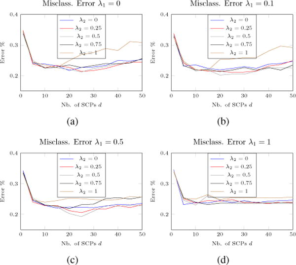
Classification error on 10-fold for various parameter values. While an initial sharp decrease in classification error can be observed with an increase of d, the error rates then reaches a plateau for the approximate range d ∈ [20, 30]. It can then be seen that a higher number of SCPs leads to a moderate increase of classification error. As a consequence, for our tests, we used (λ1, λ2, d) = (0.5,0.5,25).
Differential SCP’s are further selected using two criteria:
A stability criterion is used to assess the ‘robustness’ of each SCP component. For each of the d = 264 components within each SCP, we count how many times that component has been selected by the model (i.e., set to non zero value). If that component has been selected in at least 90% of the runs then we keep it, if not we simply discard it.
We also use a two-sample Kolmogorov-Smirnov test with a significance level α = 0.01 to test if the weight values for a given SCP across both classes follow the same distribution. If the test is positive and no significant difference is found between the two distributions, then we discard the corresponding differential SCP.
After enforcing these rules, this leaves us with a total of 3 SCP’s (indexes d ∈ {1, 2, 5}) that seem to display truly discriminative behavior across classes.
In order to facilitate the analysis of these SCP’s, we rely on the work from Smith et. al[29] and assign functional roles to some brain regions. In their work, a total of 10 resting-state maps (RSM) have been identified from 36 healthy adults at rest using ICA. Although they actually identify up to 70 meaningful components, we restrict ourselves to the 10 ‘well-matched’[29] maps. RSMs 1, 2 and 3 (visual network) correspond to medial, occipital pole, and lateral visual areas. RSM 4 corresponds to the DMN, while RSM 5 covers the cerebellum. Additional classical functions are represented in RSM 6 (sensorimotor), RSM 7 (auditory), RSM 8 (medial frontal/executive control), and RSMs 9,10 are two strongly lateralized frontoparietal maps. For each of the d = 264 nodes that our network is made of, we calculate the membership relative to each of the 10 RSM maps by considering a small sphere of 4mm radius around that node. A z-score membership can then be derived, and we chose to assign membership to a given map if a node has a z-score z > 3. We display each of these RSMs in Fig. 5 in terms of the 264 functional nodes considered in this work.
Fig. 5.
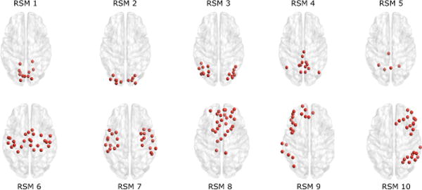
Resting state functionnal module maps defined by Smith et. al[29], expressed in the 264 nodes networks by Power et al. [9]. RSM1: Medial Visual, RSM2: Occipital Pole Visual, RSM3: Lateral Visual, RSM4: Default Mode Network, RSM5: Cerebellum, RSM6: Sensorimotor, RSM7: Auditory, RSM8: Medial Frontal/Executive Control, RSM9: Frontoparietal Right, RSM10: Frontoparietal Left.
Fig. 6(a) displays the first differential SCP defined by exclusively positive correlation values between the DMN, parts of 2 fronto-parietal maps as well as, to a lower extent, the auditory and executive control components. DMN and executive control system are often linked with complex cognitive or emotional functions. Similarly, the auditory network, responsible for auditory percpetion, has also been associated with complex cognitive functions related to language[29]. By looking at the weights histogram in Fig. 6(b), we can observe that this SCP seems to be significantly stronger within children than young adults. This seems to agree with previous work on functional connectivity between children and young adults[3]. When compared independently across populations, all DMN, Auditory System and Executive Control System nodes were reported to display increased connectivity in children compared to young adults. On the other hand, no differences were reported in both Frontoparietal networks in that study.
Fig. 6.
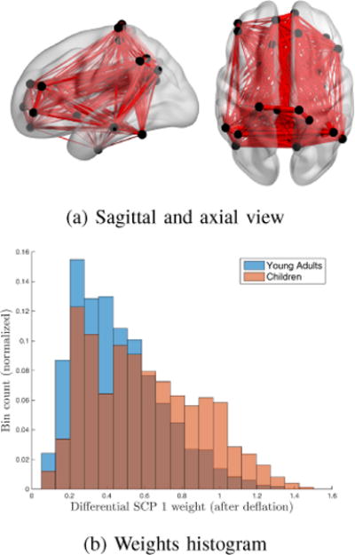
1st differential SCP (Young adults) (a) Differential edges between children and young adults (Red: positive correlation values, Blue: negative correlation values). (b) Weights of this SCP within each class.
The 2nd differential SCP can be seen in Fig. 7(a). It exhibits contributions from all 3 visual regions as well as auditory. These regions are anti-correlated with DMN, both fronto-parietal RSMs and the executive control map. Comparing once again the two histograms of Fig. 7(b) allows us to observe a much stronger expression of that SCP within young adults than children. More specifically, this SCP is assigned a near-zero weight for a significant proportion of young children. Interestingly, in the same study, Jolles et. al [3] reported an overall lower connectivity in the visual system for young children. Notice that all three visual RSMs contribute to this second differential SCP. Compared to the first differential SCP, we can observe a much more specialized and functionally ‘complex’ behavior here, where both correlated and anti-correlated components are represented. Additionally, association between regions at long distances to each other can be seen. This seems to go along with results published by previous studies[30] indicating more diffuse patterns of functional connectivity in children. As a consequence, observing much lower weights in children relative to such complex connectivity pattern should be expected.
Fig. 7.
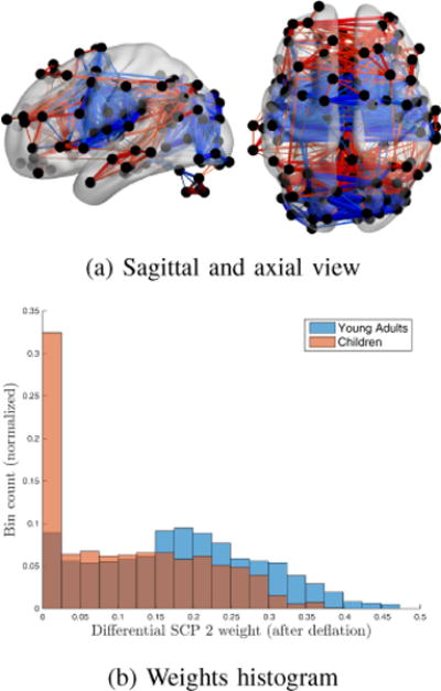
2nd differential SCP (Young adults) (a) Differential edges between children and young adults (Red: positive correlation values, Blue: negative correlation values). (b) Weights of this SCP within each class.
Finally, the 3rd differential SCP is displayed in Fig. 8(a). It shows a strong correlation between cerebellum, executive control system and medial visual RSMs . Anti-correlated regions are made of the two fronto-parietal maps. As mentioned by Fair et al.[31] in a previous study, increased associations between frontal and parietal regions develop with increased age. In their paper, they suggest that such pattern of development may be linked with learning mechanism that evolve along childhood. Although frontal and parietal cortices do display a certain amount of connectivity in children, this phenomenon increases significantly with age. Additionally, this connectivity pattern can be described as fairly complex as well, which might explain why it is significantly more expressed in young adults than in children.
Fig. 8.
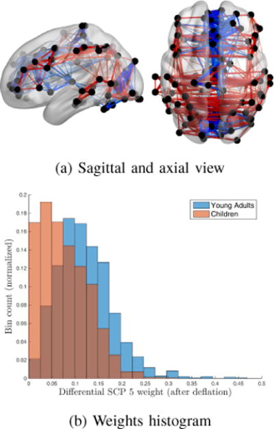
3rd differential SCP (Young adults) (a) Differential edges between children and young adults (Red: positive correlation values, Blue: negative correlation values). (b) Weights of this SCP within each class.
3) Comparison with other methods
Although achieving the best classification accuracy is not the main goal of this paper, we do rely on such measure in order to: (i) estimate parameter values (ii) assess whether or not the differential components of the extracted SCP display a discriminative behavior. Furthermore, can also compare the classification accuracies obtained with the proposed method with the following alternate approaches from the literature:
Joint-SVM: the proposed method followed by a classification step using standard linear SVM.
Separate-SVM: the proposed method without the joint penalty (i.e. λ2 = 0) followed by a classification step.
CorrMat-SVM: using the full correlation matrix as a feature in the classification step.
PCA-SVM: supervised PCA analysis followed by a classification step using the associated coefficients.
ICA-SVM: ICA group analysis (for each class) using GIFT toolbox3 followed by classification using the total absolute connectivity values as subject-wise features.
In Fig. 9, we display the classification accuracy average over a 10-fold cross validation for each of these methods. We can observe that standard PCA performs rather poorly. Our proposed joint model provides the second best performances after using the full correlation matrix as a feature. The authors would like to point out that relying on the full correlation matrix amounts to consider 34716 features, while for our joint model we only consider 2 × d = 50 features for the classification step. Such 500-fold decrease in the number of features, while slightly damaging the overall classification accuracy, leads to a much easier interpretability of the results.
Fig. 9.
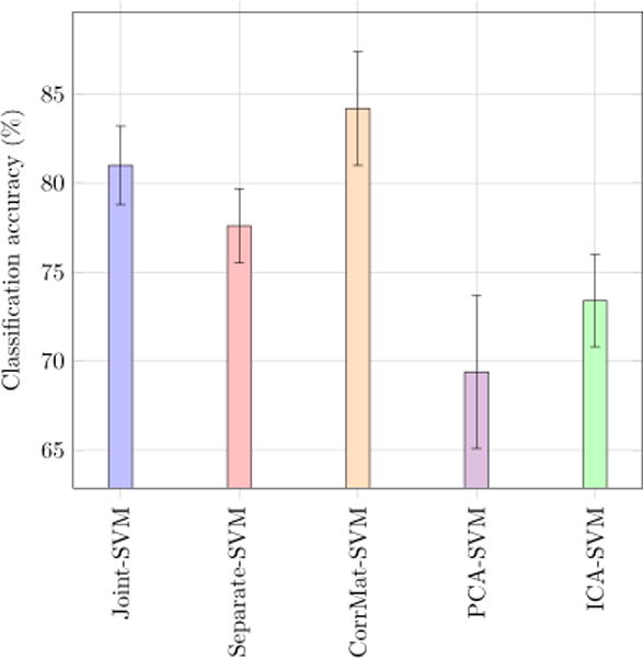
Classification accuracy (%) and and associated standard deviation (black lines) values for 5 different methods using a SVM classifier.
IV. Discussion and Conclusion
The work presented in this paper evaluates functional connectivity differences between children and young adults. More specifically, we estimate functionally coherent sets of brain regions, called SCP’s, on the basis of their behaviors during the resting state. In addition, we pay special attention to identifying both shared and class-specific connectivity patterns between these two populations. In order to do so, we extend previous work from Eavani et al.[6] and propose a new data-driven approach for multi-class set-ups. We then enforce the hypothesis that the two classes considered share, to a certain degree, similar patterns of functional brain activity by using a fused Lasso penalty. Such an assumption may prove to be particularly useful in studies where sample number is low, as it allows the user to harness the power of each different class, instead of requiring a separate analysis.
The objective of our simulated experiments was to validate the use of the fusion penalty. More specifically, we wanted to see if a mix of ℓ1 and fused norm could significantly increase the analysis power in a multi-class setup. In our opinion, the results on the simulated data sumed up in Fig. 3(a)–(c) did show that combining both sparsity and fusion across classes can drastically improve the estimation process compared to a standard non-sparse (λ1 = 0) class-wise (λ2 = 0) approach. The benefits of the fused term are obvious when it comes to estimate truly shared components. It is interesting as well to note that such regularization term can also (assuming a proper estimation of the parameter λ2 has been performed) improve the estimation (in terms of feature selection accuracy) of the differential components (c.f. Fig. 3(d)–(f)). Finally, it also leads to a lower classification error on the real data when using the weight maps associated to the differential SCP components, as seen in Fig. 4. One explanation could be that a more accurate estimation of the shared component makes it easier for the algorithm to properly identify class-specific components.
We then used our fused model to estimate differential SCP’s between children and young adults with a fairly large number of samples (n = 583 here). Three of these SCP’s were made of components identified as class-specific/differentials. The first differential SCP is made of exclusively positive correlation across several functional systems where increased activity in children compared to young adults have been observed before by a similar study[3]. On the other hand, one can observe that differential connectivity patterns 2 and 3 are fairly more complex than the first one. On top of that, they are both significantly more expressed in young adults than in children. It has been previously reported[3], [30] that overall, children’s brains shows more diffuse, less specialized activity patterns, as well as a lower expression of long range interactions between distant regions, which is consistent with our observations.
One potential limitation of this approach has already been mentioned by Eavani et al.[6]. Namely, the use of a single value for the sparsity parameter λ1 might prove sub-optimal when the estimated SCP’s have different sizes (i.e. different numbers of non-zeros components). A similar remark can be made about the fused term regularization parameter λ2 in the case of unbalanced class. Additional experiments should be carried out to examine the effect of having one class composed of significantly more data samples than the other. One can try to give more freedom to the algorithm by allowing different λ1, λ2 values for each SCP/class, but gridsearch-like parameter estimation scheme quickly becomes intractable. Similarly, the use of the fused penalty with more than 2 classes in the case of high dimensional data needs to be carefully addressed in terms of computational complexity. Finally, another research direction may be in comparing the fused penalty with other joint penalties such as, e.g., group-based penalty[32], since connected patterns usually form a group in the brain region. In conclusion, we have proposed a model to extract sparse co-activated sub-networks from fMRI images in a multi-class setup. Using simulations and real data, we have demonstrated that this method can efficiently identify both shared and class-specific variables. We hope this model provides an accurate and powerful tool for extracting connectivity patterns among populations.
Supplementary Material
Acknowledgments
The work was partially supported by NIH (R01 GM109068, R01 MH104680, R01 MH107354, P20 GM103472, R01 REB020407, 1R01 EB006841) and NSF (#1539067).
Footnotes
References
- 1.Friston KJ. Functional and effective connectivity: a review. Brain connectivity. 2011;1(1):13–36. doi: 10.1089/brain.2011.0008. [DOI] [PubMed] [Google Scholar]
- 2.Fair DA, Cohen AL, Power JD, Dosenbach NU, Church JA, Miezin FM, Schlaggar BL, Petersen SE. Functional brain networks develop from a local to distributed organization. PLoS comput biol. 2009;5(5):e1000381. doi: 10.1371/journal.pcbi.1000381. [DOI] [PMC free article] [PubMed] [Google Scholar]
- 3.Jolles DD, Buchem MAvan, Crone EA, Rombouts SA. A comprehensive study of whole-brain functional connectivity in children and young adults. Cerebral Cortex. 2011;21(2):385–391. doi: 10.1093/cercor/bhq104. [DOI] [PubMed] [Google Scholar]
- 4.Passarotti AM, Paul BM, Bussiere JR, Buxton RB, Wong EC, Stiles J. The development of face and location processing: An fmri study. Developmental Science. 2003;6(1):100–117. [Google Scholar]
- 5.Holland SK, Plante E, Byars AW, Strawsburg RH, Schmithorst VJ, Ball WS. Normal fmri brain activation patterns in children performing a verb generation task. Neuroimage. 2001;14(4):837–843. doi: 10.1006/nimg.2001.0875. [DOI] [PubMed] [Google Scholar]
- 6.Eavani H, Satterthwaite TD, Filipovych R, Gur RE, Gur RC, Davatzikos C. Identifying sparse connectivity patterns in the brain using resting-state fmri. Neuroimage. 2015;105:286–299. doi: 10.1016/j.neuroimage.2014.09.058. [DOI] [PMC free article] [PubMed] [Google Scholar]
- 7.De LM, Beckmann C, De SN, Matthews P, Smith S. fmri resting state networks define distinct modes of long-distance interactions in the human brain. Neuroimage. 2006;29:1359–1367. doi: 10.1016/j.neuroimage.2005.08.035. [Online]. Available: [DOI] [PubMed] [Google Scholar]
- 8.Calhoun VD, Kiehl KA, Pearlson GD. Modulation of temporally coherent brain networks estimated using ica at rest and during cognitive tasks. Human brain mapping. 2008;29(7):828–838. doi: 10.1002/hbm.20581. [DOI] [PMC free article] [PubMed] [Google Scholar]
- 9.Power JD, Cohen AL, Nelson SM, et al. Functional network organization of the human brain. Neuron. 2011;72(4):665–678. doi: 10.1016/j.neuron.2011.09.006. [DOI] [PMC free article] [PubMed] [Google Scholar]
- 10.Tzourio-Mazoyer N, Landeau B, et al. Automated anatomical labeling of activations in spm using a macroscopic anatomical parcellation of the mni mri single-subject brain. Neuroimage. 2002;15(1):273–289. doi: 10.1006/nimg.2001.0978. [DOI] [PubMed] [Google Scholar]
- 11.Allen EA, Erhardt EB, Damaraju, et al. A baseline for the multivariate comparison of resting-state networks. Frontiers in systems neuroscience. 2011;5:2. doi: 10.3389/fnsys.2011.00002. [DOI] [PMC free article] [PubMed] [Google Scholar]
- 12.Cao J, Worsley K, et al. The geometry of correlation fields with an application to functional connectivity of the brain. The Annals of Applied Probability. 1999;9(4):1021–1057. [Google Scholar]
- 13.Smith SM, Miller KL, Salimi-Khorshidi, et al. Network modelling methods for fmri. Neuroimage. 2011;54(2):875–891. doi: 10.1016/j.neuroimage.2010.08.063. [DOI] [PubMed] [Google Scholar]
- 14.Li X, Wang H. Identification of functional networks in resting state fmri data using adaptive sparse representation and affinity propagation clustering. Frontiers in neuroscience. 2015;9 doi: 10.3389/fnins.2015.00383. [DOI] [PMC free article] [PubMed] [Google Scholar]
- 15.Calhoun VD, Liu J, Adali T. A review of group ica for fmri data and ica for joint inference of imaging, genetic, and erp data. NeuroImage. 2009;45(1, Supplement 1):S163–S172. doi: 10.1016/j.neuroimage.2008.10.057. mathematics in Brain Imaging. [DOI] [PMC free article] [PubMed] [Google Scholar]
- 16.Anderson A, Douglas PK, Kerr WT, et al. Non-negative matrix factorization of multimodal mri, fmri and phenotypic data reveals differential changes in default mode subnetworks in adhd. NeuroImage. 2014;102:207–219. doi: 10.1016/j.neuroimage.2013.12.015. [DOI] [PMC free article] [PubMed] [Google Scholar]
- 17.Lee DD, Seung HS. Algorithms for non-negative matrix factorization. Advances in neural information processing systems. 2001:556–562. [Google Scholar]
- 18.Leonardi N, Richiardi J, Gschwind M, Simioni S, Annoni J-M, Schluep M, Vuilleumier P, Van De Ville D. Principal components of functional connectivity: a new approach to study dynamic brain connectivity during rest. NeuroImage. 2013;83:937–950. doi: 10.1016/j.neuroimage.2013.07.019. [DOI] [PubMed] [Google Scholar]
- 19.Yang M, Zhang L, Feng X, Zhang D. Fisher discrimination dictionary learning for sparse representation; Computer Vision (ICCV), 2011 IEEE International Conference on; IEEE; 2011. pp. 543–550. [Google Scholar]
- 20.Eavani H, Satterthwaite TD, Gur RE, Gur RC, Davatzikos C. Discriminative Sparse Connectivity Patterns for Classification of fMRI Data. Springer International Publishing; 2014. pp. 193–200. [DOI] [PMC free article] [PubMed] [Google Scholar]
- 21.Satterthwaite TD, Connolly JJ, Ruparel K, Calkins ME, Jackson C, Elliott MA, Roalf DR, Hopsona KPR, Behr M, Qiu H, et al. The philadelphia neurodevelopmental cohort: a publicly available resource for the study of normal and abnormal brain development in youth. Neuroimage. 2016;124:1115–1119. doi: 10.1016/j.neuroimage.2015.03.056. [DOI] [PMC free article] [PubMed] [Google Scholar]
- 22.Danaher P, Wang P, Witten DM. The joint graphical lasso for inverse covariance estimation across multiple classes. Journal of the Royal Statistical Society: Series B (Statistical Methodology) 2014;76(2):373–397. doi: 10.1111/rssb.12033. [DOI] [PMC free article] [PubMed] [Google Scholar]
- 23.Fang J, Lin D, Schulz C, Xu Z, Calhoun VD, Wang Y-P. Joint sparse canonical correlation analysis for detecting differential imaging genetics modules,” Bioinformatics, 2016. doi: 10.1093/bioinformatics/btw485. [DOI] [PMC free article] [PubMed] [Google Scholar]
- 24.Boyd S, Parikh N, Chu E, Peleato B, Eckstein J. Distributed optimization and statistical learning via the alternating direction method of multipliers. Foundations and Trends in Machine Learning. 2011;3(1):1–122. [Google Scholar]
- 25.Friedman J, Hastie T, Höfling H, Tibshirani R, et al. Pathwise coordinate optimization. The Annals of Applied Statistics. 2007;1(2):302–332. [Google Scholar]
- 26.Cortes C, Vapnik V. Support-vector networks. Machine learning. 1995;20(3):273–297. [Google Scholar]
- 27.Erhardt EB, Allen EA, Wei Y, Eichele T, Calhoun VD. Simtb, a simulation toolbox for fmri data under a model of spatiotemporal separability. NeuroImage. 2012;59(4):4160–4167. doi: 10.1016/j.neuroimage.2011.11.088. [DOI] [PMC free article] [PubMed] [Google Scholar]
- 28.Satterthwaite TD, Elliott MA, Ruparel, et al. Neuroimaging of the philadelphia neurodevelopmental cohort. Neuroimage. 2014;86:544–553. doi: 10.1016/j.neuroimage.2013.07.064. [DOI] [PMC free article] [PubMed] [Google Scholar]
- 29.Smith SM, Fox PT, Miller KL, Glahn DC, Fox PM, Mackay CE, Filippini N, Watkins KE, Toro R, Laird AR, et al. Correspondence of the brain’s functional architecture during activation and rest. Proceedings of the National Academy of Sciences. 2009;106(31):13 040–13 045. doi: 10.1073/pnas.0905267106. [DOI] [PMC free article] [PubMed] [Google Scholar]
- 30.Kelly AC, Martino ADi, Uddin LQ, Shehzad, et al. Development of anterior cingulate functional connectivity from late childhood to early adulthood. Cerebral cortex. 2009;19(3):640–657. doi: 10.1093/cercor/bhn117. [DOI] [PubMed] [Google Scholar]
- 31.Fair DA, Dosenbach NU, Church JA, Cohen AL, Brahmbhatt S, Miezin FM, Barch DM, Raichle ME, Petersen SE, Schlaggar BL. Development of distinct control networks through segregation and integration. Proceedings of the National Academy of Sciences. 2007;104(33):13 507–13 512. doi: 10.1073/pnas.0705843104. [DOI] [PMC free article] [PubMed] [Google Scholar]
- 32.Simon N, Friedman J, Hastie T, Tibshirani R. A sparse-group lasso. Journal of Computational and Graphical Statistics. 2013;22(2):231–245. [Google Scholar]
Associated Data
This section collects any data citations, data availability statements, or supplementary materials included in this article.


