Recent Activity in Expanding Populations and Purifying Selection Have Shaped Transposable Element Landscapes across Natural Accessions of the Mediterranean Grass Brachypodium distachyon

Abstract

Transposable element (TE) activity has emerged as a major cause of variation in genome size and structure among species. To what extent TEs contribute to genetic variation and divergence within species, however, is much less clear, mainly because population genomic data have so far only been available for the classical model organisms. In this study, we use the annual Mediterranean grass Brachypodium distachyon to investigate TE dynamics in natural populations. Using whole-genome sequencing data for 53 natural accessions, we identified more than 5,400 TE polymorphisms across the studied genomes. We found, first, that while population bottlenecks and expansions have shaped genetic diversity in B. distachyon, these events did not lead to lineage-specific activations of TE families, as observed in other species. Instead, the same families have been active across the species range and TE activity is homogeneous across populations, indicating the presence of conserved regulatory mechanisms. Second, almost half of the TE insertion polymorphisms are accession-specific, most likely because of recent activity in expanding populations and the action of purifying selection. And finally, although TE insertion polymorphisms are underrepresented in and around genes, more than 1,000 of them occur in genic regions and could thus contribute to functional divergence. Our study shows that while TEs in B. distachyon are “well-behaved” compared with TEs in other species with larger genomes, they are an abundant source of lineage-specific genetic variation and may play an important role in population divergence and adaptation.

Introduction

When in the 17th century Antonie van Leeuwenhoek focused his microscope on objects of everyday life, he discovered a microcosm that was unknown to people at the time. In a similar way, our increasing ability to zoom in on the genomes of organisms has revealed a complexity unsuspected two decades ago. Far from being mere instructions on how to construct and maintain an organism, the genomes of eukaryotes are populated by a large amount of “animalcules” known as transposable elements (TEs), that is, selfish stretches of DNA which can replicate within genomes (Burt and Trivers 2006).

TEs capable of replication carry at least promoter sequences and, if autonomous, also open reading frames encoding the transposition machinery. In the simplest case, the insertion of such sequences across the genome disrupts functional elements (e.g. Mendel’s wrinkled peas, Bhattacharyya et al. 1990). More subtle effects at the regulatory level include the creation of alternative or new promoters (reviewed in Feschotte 2008) and the alteration of epigenetic landscapes (reviewed in Slotkin and Martienssen 2007; Lisch 2009). And at the structural level, the spread of highly similar sequences across chromosomes provides the substrate for ectopic recombination and structural rearrangements, including the deletion and duplication of genes (Xiao et al. 2008; Gordon et al. 2017).

Although TEs are powerful mutagens, their role in the evolution of natural populations has been little explored. Most of our knowledge about TEs stems from top-down approaches, that is, approaches starting from phenotypic variation and searching for the causative mutation. Such studies have revealed fascinating molecular details of how TEs can change single host traits in a range of organisms (Casacuberta and González 2013; Lisch 2013; van’t Hof et al. 2016). To understand the evolutionary dynamics of TEs, however, requires insights into their molecular behavior as well as into the microevolutionary processes which eventually determine their success or failure in natural populations (Tenaillon et al. 2010; Bonchev and Parisod 2013). Population size, in particular, is an important factor in genome evolution and TE dynamics (Lynch 2007), as it determines how efficiently selection can oppose the accumulation of deleterious TE insertions. Indeed TEs seem to thrive in small, stressed populations where the efficacy of purifying selection is reduced, as studies on bottlenecked invasive and endangered species (Schrader et al. 2014; Abascal 2016) as well as on natural plant populations (Lockton et al. 2008) have shown.

Bottom-up population genomic approaches promise to provide a more complete picture of the evolutionary dynamics of TEs in natural populations. In Drosophila, the best studied organism in this regard, studies using population-genomic data found that some TE families underwent bursts of transposition during the expansion of D. melanogaster and D. simulans out of Africa (Kofler et al. 2015) and played a role in the adaptation of D. melanogaster to temperate climate (González et al. 2008, 2010; Merenciano et al. 2016). In addition, they substantiated previous claims that purifying selection against TEs acts primarily against the deleterious effects of ectopic recombination (Petrov et al. 2003, reviewed in Barrón et al. 2014).

Despite the abundance and diversity of TEs in plants, there has been no comparable effort to understand TE evolution in wild populations within this diverse kingdom. Research on TE polymorphisms in plants has largely focused on crops (reviewed in Vitte et al. 2014) and questions regarding the chromosomal distribution of TEs (Tian et al. 2012; Sanseverino et al. 2015; Wei et al. 2016; Lai et al. 2017) or the effect of TE insertions on gene expression and methylation patterns (Makarevitch et al. 2015; Quadrana et al. 2016; Stuart et al. 2016). The most comprehensive study on TE dynamics in natural populations remains the classical study on Arabidopsis lyrata by Lockton et al. (2008) which, using a TE display approach, found that selection against TEs is reduced in bottlenecked populations. To our knowledge, there is so far no genome-wide investigation of TE polymorphisms which explicitly considers population structure and demographic history in wild plant populations.

The primary reason for this knowledge gap is the scarcity of high-quality reference genomes for noncrop species, as the investigation of TE evolution in natural populations requires reference-based approaches. In this study, we took advantage of the near base-perfect reference genome (latest version available on https://phytozome.jgi.doe.gov) of the wild grass Brachypodium distachyon to study the microevolutionary dynamics of TEs. Brachypodium distachyon occurs around the Mediterranean in arid, oligotrophic habitats with recurring disturbance. Established as a powerful functional genomics resource for the grasses (reviewed in Brutnell et al. 2015), its reference genome is entirely assembled in five chromosomes (272 megabases) and has been annotated for genes and TEs (International Brachypodium Initiative 2010). In line with what has been found in other plants, retrotransposons represent the majority of TEs in the reference genome, both in terms of copy number (50,419) and contribution to genome size (23%, International Brachypodium Initiative 2010). DNA transposons, on the other hand, constitute about 5% of the genome. Since highly repetitive regions of the genome could be assembled through the use of BAC libraries (International Brachypodium Initiative 2010; VanBuren and Mockler 2016), B. distachyon constitutes a prime system to investigate TE evolution with a reference-based approach.

Using whole-genome sequencing data for 53 natural accessions originating mainly from Spain and Turkey (Gordon et al. 2017), we here investigated genome-wide TE polymorphisms in the light of the demographic history of B. distachyon populations. We were particularly interested in addressing the following questions. First, are TEs still active in this small-genome species and, if yes, which families are active? Second, are there lineage-specific proliferations of TE families which correlate with demographic events such as bottlenecks or expansions? And finally, how does purifying selection affect the distribution of TE polymorphisms?

Materials and Methods

Biological Material and SNP Calling

The genomes of the 53 B. distachyon accessions analyzed in this study were recently sequenced at a mean coverage of 74 to create a B. distachyon pan-genome (supplementary table S1, Supplementary Material online; Gordon et al. 2017). For each accession, we aligned the 76 or 100 bp Illumina paired-end reads with BWA-MEM (standard settings, Li 2013) to version 2.0 of the B. distachyon reference genome. After removing duplicates with Sambamba (Tarasov et al. 2015), single nucleotide polymorphisms were called with Freebayes (Garrison and Marth 2012). Standard settings were used for both programs. The following filters were applied to the raw Freebayes output: we first removed indels and variants in low complexity regions identified with Dustmasker (Morgulis et al. 2006). VCFtools v0.1.12b (Danecek et al. 2011) was then used to remove SNPs with a quality lower than 30 and a mean depth lower than half or higher than twice the genome-wide average depth at all variant sites. This filtered data set with 5,918,789 SNPs will be referred to as the full SNP data set; further filtering steps were adapted to the requirements of the different methods and are described below.

Genetic Structure, Nucleotide Diversities, and Phylogenetic Tree Estimation

To assess the genetic structure in the 53 accessions, we LD-pruned the full SNP data set with Plink 1.9 (–indep-pairwise 50 10 0.1, Purcell et al. 2007) and removed sites with missing genotypes and minor allele frequencies (MAF) lower than 0.05 in order to obtain an informative set of unlinked SNPs. With the resulting 145,576 SNPs, a principal component analysis (PCA) was conducted using the snpgdsPCA function in the R package SNPrelate (Zheng et al. 2012). The program Admixture (Alexander et al. 2009) was used with the same data to identify potential admixture between the three genetic clusters. The analysis was run for K values from 1 to 5, and the best model was determined as the model with the lowest cross-validation error, as suggested by the authors of the algorithm. A measure of the genetic distance between the three clusters was obtained by computing pairwise nucleotide differences (Hudson et al. 1992; Wakeley 1996) between and within clusters using the PopGenome package in R (Pfeifer et al. 2014) and the full SNP data.

A phylogenetic tree was estimated with the program SNPhylo (Lee et al. 2014), using the full SNP data because LD pruning is performed by the program. Brachypodium stacei, a closely related species of B. distachyon, was included as outgroup. To do so, we downloaded B. stacei short reads from the NCBI database (SRR1800497–SRR1800504), aligned them to the B. distachyon reference genome, called SNPs for B. stacei with Freebayes at the already called SNP sites (−l@ parameter), and added the variants to the original vcf file. 100 bootstrap replicates were performed to assess the consistency of the tree.

Demographic Inference

The sequential Markov coalescent implemented in SMC++ (Terhorst et al. 2017) was used to estimate the demographic history of B. distachyon populations. This program runs on unphased SNP data and exploits linkage disequilibrium information across the genome to infer ancestral population sizes. Compared with previous LD-based methods, it allows the inclusion of more individuals and yields more accurate estimates especially for recent demographic history (Terhorst et al. 2017). Because population substructure can result in spurious signals of population expansions or bottlenecks (Mazet et al. 2016), the analysis was conducted separately for eastern and western relict accessions. In addition, we excluded four Spanish and four Iraqi accessions which show signs of admixture in the Admixture analysis (see below), as well as chromosome 5 because of long runs of homozygosity. For each genetic cluster, two accessions were randomly chosen for each of the four remaining chromosomes and used as distinguished lineages to calculate composite likelihoods, using the full SNP data set. A polarization error of 0.5 was set because we did not determine the identity of the ancestral alleles. Finally, a mutation rate of 7e−9 per site per generation (estimate for Oryza sativa, Lynch et al. 2016) was assumed to translate coalescence times into generations.

Detection of Transposable Element Polymorphisms

Transposable element insertion polymorphisms (TIPs)—that is, TEs present in a sampled accession but absent from the reference—were identified with TEMP (Zhuang et al. 2014), using version 2.0 the B. distachyon reference genome and B. distachyon TE consensus sequences from the TREP database (http://botserv2.uzh.ch/kelldata/trep-db/index.html). TEMP uses discordant read pairs in which one read aligns uniquely to the reference genome and its mate does not, but rather aligns to the consensus sequence of a TE. In a further step, split reads spanning the TE insertion boundaries are used to obtain the position of the insertion. The notion of unique mapping is crucial to the discordant read-pair approach, as it implies that an “anchor” can be placed in the reference genome. We defined a uniquely mapping read as one where the mapping score of the second best hit was at least 30 lower than the score of the best hit. With a standard mismatch penalty of 6, this means that the second best hit had at least five more mismatches than the best hit.

The detection of TE absence polymorphisms (TAPs), on the other hand, requires an annotation of TEs in the reference genome. As such an annotation was only available for version 1 of the reference assembly, we transferred the available annotation to the reference assembly v.2.0 with RATT (Otto et al. 2011). Only 187 out of 90,661 TEs and TE fragments could not be transferred, which agrees with the minor changes in the newer assembly. In the absence analysis, TEMP first identifies all paired-end reads which show an increased insert size compared with the expectation. In a second step, TEMP assesses whether the identified reads are spanning an annotated TE and, if yes, whether the deviation from the expected insert size corresponds to the length of the annotated TE.

As TEMP was originally designed for analyzing pooled sequencing data, and in order to reduce the number of false positives, stringent filtering criteria were applied to the raw output of the program. First, we included only TIPs which were supported from both the 5′ and the 3′ side. Second, we required a proportion of reads supporting a TIP against all reads mapping to the region of at least 0.3. This arbitrary value was chosen to account for heterozygous insertions and a possible imbalance of the number of reads derived from two homologous chromosomes. For the absence analysis, we required a proportion of reads supporting a TAP of at least 0.9. As a last filtering step for both analyses, TE variants were excluded if they had abnormally low or high coverages. To define the thresholds for this filtering step, we took the distribution of coverages for the TE variants, which approximates the distribution of sequencing depth across the genome, and defined an outlier as a point outside the interval [Q1− 1.5× IQR, Q3 + 1.5×IQR], with Q1 and Q3 being the first and third quartile of the distribution and IQR the interquartile range Q3− Q1. This is the outlier definition normally used in boxplots. This filtering step allowed eliminating noise due to genomic regions with high complexity or insufficient coverage. The filtered TEMP results were finally converted into presence/absence matrices. We considered a TE insertion identical across accessions and originating from the same insertion event if it was detected in the same 50-bp window and if the same TE family was identified.

Downsampling Analysis

To estimate the effect of sequencing coverage on the ability of TEMP to detect TE polymorphisms, we performed a downsampling analysis. The coverage of ten high-coverage accessions was downsampled in steps of 10% using the DownsampleSam function of Piccard Tools version 1.97 (https://broadinstitute.github.io/picard/). TEMP was then run with the read subsets thus obtained. Plotting the number of discovered TIPs/TAPs against coverage indicated that a logistic growth curve could model the relationship between these two variables. Self-starting nonlinear least squares models were fitted in R with the nls and the SSlogis functions. Interpreting the asymptotes of the logistic growth curves as the maxima of detectable TE variants, we calculated for each of the ten downsampled accessions the coverage needed to attain 95% of the maximally detectable variants. Finally, we took the average of the ten results obtained in the previous step, which gave an estimate of the average coverage depth needed to find 95% of the detectable TIPs and TAPs.

SNP Allele Frequency Spectra

In this study, TE variants were treated as dominant markers, that is, information about heterozygosity was not taken into account. To allow a direct comparison of observed SNP and TIP/TAP frequencies, SNPs were treated as dominant markers as well: SNPs were scored as present regardless of whether they are homo- or heterozygous. We used the full SNP data set (no MAF-filtering, see above), but only considered SNPs located in nongenic regions because these are more likely to be neutral than SNPs in genic regions and thus better reflect the effects of demographic history. Since most TIPs and TAPs are likely due to recent events and thus represent derived mutations (see below), we polarized the SNP data to make the TIP, TAP, and SNP frequency spectra more comparable. To do so, the aligned B. stacei reads described above were used and the B. stacei allele was assumed to represent the ancestral state. In this way, we obtained 1,275,199 polarized SNPs for the eastern cluster, 1,369,271 for the western cluster, and 1,518,262 for the relict cluster.

Statistical Analyses

A multivariate analysis of variance was conducted in order to assess whether TE families show different activities across genetic clusters. To do so, the relative abundance of each TE family was used to calculate a matrix of Euclidian distance among accessions. This matrix was then entered as the dependent variable and the genetic cluster as an explanatory variable in a linear model using the adonis function of the R package vegan (Oksanen et al. 2017).

To test whether the genetic cluster of origin had an effect on the number of detected TIPs, a phylogenetic generalized least squares (GLS) regression was performed using the R package nlme (Pinheiro et al. 2017). We first randomly extracted 50,000 SNP from our SNP data set. This subset was then used to calculate phylogenetic distances among accessions with the R package pvclust (Suzuki and Shimodaira 2006). Phylogenetic distances were integrated in a GLS by specifying a phylogenetic correlation structure according to a Brownian motion model (Felsenstein 1985); the number of TIPs per accession was set as response variable and the genetic cluster as explanatory variable. In addition, we used the “weights” argument in the gls function to allow for different variances across genetic clusters, in order to attenuate heteroscedasticity (Zuur et al. 2009).

The correlation between SNPs and TIPs was estimated with the mantel.rtest function in ade4 (Dray and Dufour 2007). The genetic distance matrix for SNPs was created with the snpgdsIBS function from SNPrelate, while we used the Jaccard index to calculate the genetic distance matrix for TIPs, as implemented in the vegdist function of vegan (Oksanen et al. 2013). 1,000 bootstrap replicates were performed to assess the significance of the correlation. All other basic statistical analyses and graphics were conducted in R, version 3.1.3.

Genomic Context Analysis

We used the reference annotation version 2.1 to determine the position of the identified TIPs with regard to genes. Six categories were defined: within exons, within introns, within the 3′ UTR, the 5′ UTR, within 2 kb of a gene, and intergenic. Each TIP was assigned to a category. To determine the statistical significance of the observed number of TIPs in each category, we used the exact Poisson test in R to obtain the probability of the observed value under a random insertion model according to which the proportion of TIPs in a category corresponds to the proportion of base pairs in the reference genome that fall into this category.

Results and Discussion

Population Bottlenecks and Expansions have Shaped Genetic Diversity in B. distachyon

This study is based on whole-genome sequencing data for 53 natural accessions of B. distachyon which mainly originate from Turkey and Spain (fig. 1A;supplementary table S1, Supplementary Material online; Gordon et al. 2017). Using Illumina paired-end reads with a mean sequencing coverage of 74 per genome, we identified more than five millions single nucleotide polymorphisms (SNPs) across the sampled accessions. In order to get a first picture of the genetic structure in these samples, we conducted a PCA with a LD-pruned subset of 145,576 SNPs. The results show that the 53 accessions form three genetic clusters: an eastern cluster (27 accessions from Turkey and Iraq, including the reference accession Bd21), a western cluster (17 accessions from Spain and France), and a third, more spread-out cluster with five individuals from Turkey, the accession from the Crimea, the accession from Slovenia, and two accessions from Spain (fig. 1A and B). A rooted maximum likelihood tree based on SNP data, with the closely related B. stacei as outgroup, confirms the presence of three highly supported monophyletic groups and reveals an ancestral split between the spread-out cluster and the two others (fig. 2). Levels of admixture between the clusters appear to be low, as suggested by an Admixture analysis according to which a model with three ancestral populations best fits the data (fig. 2), and as already shown by Gordon et al. (2017). We further obtained a measure of the evolutionary distance between the three clusters by comparing pairwise nucleotide differences within and between clusters. The results show that the western and the eastern cluster harbor similar levels of genetic diversity and are more similar to each other than to the spread-out cluster (fig. 1C). Moreover, the distribution of pairwise nucleotide differences in the spread-out cluster is bimodal and covers a large range of values; high values around 0.004 are due to comparisons of the two Spanish accessions (Arn1, Mon3) with the other accessions in this cluster, suggesting the presence of population substructure.

Fig. 1.

—Sample origin and genetic structure. (A) Geographical origin of the 53 accessions analyzed in this study. Colors depict the genetic cluster, identified in the Admixture analysis, to which the accessions belong (blue: west, orange: east, gray: relicts). Numbers indicate how many accessions stem from the same place, and the * shows the origin of the reference accession Bd21. (B) Principal component analysis with 145,576 LD-pruned SNPs, with the percentage of variance explained in brackets. (C) Distribution of pairwise nucleotide diversity (π) within and between clusters.

Fig. 2.

—Phylogenic relationships and Admixture analysis. The color code is the same as in figure 1. The numbers next to the nodes show bootstrap support out of 100 replications. The reference Bd21 and the outgroup B. stacei are highlighted in bold.

The partial discrepancy between geographic origin and genetic relatedness described above has been observed in previous studies conducted in B. distachyon, both at a smaller spatial scale within Turkey (Vogel et al. 2009; Dell’Acqua et al. 2014) and in a recent survey with plants from all over southern Europe (Tyler et al. 2016). Long-distance seed dispersal and high selfing rates can lead to the local co-occurrence of highly diverged individuals (Stebbins 1957; Vogel et al. 2009). This, however, is an unlikely explanation for the large-scale patterns described above and by Tyler et al. (2016). Descendants of a long-distance dispersal event are expected to be closely related to individuals from the source population, while we observe here deep genetic divergence between the geographically separated accessions in the spread-out cluster (figs. 1C and 2).

An alternative explanation is that the nine spread-out accessions descend from relict populations, that is, they are remnants of an ancient range expansion during a period of favorable conditions (Hampe and Jump 2011; Nieto Feliner 2014), while the accessions of the eastern and the western cluster are the descendants of a highly successful lineage which has colonized large areas of the species’ range in more recent times. A similar relict scenario has been described in A. thaliana (1001 Genomes Consortium 2016), where climate relicts are characterized by deep genetic divergence and smaller effective population sizes than the highly successful lineage which has spread across the globe as a human commensal (Lee et al. 2017).

To test the relict scenario and get a more precise idea of the demographic history of B. distachyon, we used the sequential Markov coalescent method implemented in SMC++ (Terhorst et al. 2017) to infer ancestral population sizes. This analysis indicates that there has been a general decline in population size during the Quaternary glaciations from about 1 million to 30,000 years ago (fig. 3). At his point, population histories start to diverge. The ancestral putative relict populations show signs of comparatively weak bottlenecks followed by stable population sizes until present. The eastern and western ancestral populations, on the other hand, both expanded in the recent past. Interestingly, a marked bottleneck precedes the expansion of the ancestral western population, while no such severe event occurred in the ancestral eastern population.

Fig. 3.

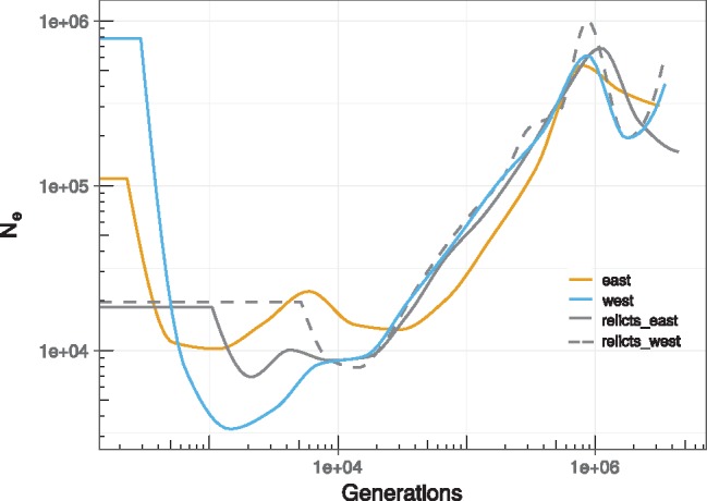
—Demographic history. Because B. distachyon is annual, the generation time directly translates into years. Again, the color code is the same as in figure 1.

These results agree with the relict scenario proposed above. Bottlenecks would explain why genetic structure is strong (fig. 2) despite the evidence that the studied lineages diverged recently, probably during the last Ice Age (fig. 3; Tyler et al. 2016). In addition, the occurrence of bottlenecks accords with the ecological niche of B. distachyon, which is a predominantly selfing specialist of disturbed habitats and might rely on the colonization of new habitats—a process which often implies strong founder effects (Stebbins 1953; Pannell 2015). On the other side, recent lineage expansions would explain the weak genetic structure (fig. 2) and comparatively low levels of genetic diversity (fig. 1C) within the eastern and the western cluster. Finally, the severe bottleneck observed in the western ancestral population suggests that the 17 accessions from Spain and France descend from a small number of genotypes that have been introduced to the western Mediterranean region and spread successfully over large areas after the last glaciation.

A mechanism of reproduction isolation between relicts and nonrelicts has already been described: flowering-time measurements in the greenhouse show that relict lineages require extended vernalization and flower significantly later than nonrelict lineages (Tyler et al. 2016, Gordon et al. 2017). This phenological difference may form a prezygotic reproductive barrier and prevent interbreeding between locally co-occurring relict- and nonrelict plants. Relicts and nonrelicts can still be crossed in the lab (Wilson et al. 2016), however, and do therefore not qualify as different species according to Mayr’s biological species concept (Mayr 1942).

With only one sample from the central Mediterranean region (Bd29-1 from Slovenia), a huge gap remains in our understanding of the distribution of genetic variation in B. distachyon. It is clear, however, that evolutionary trajectories within B. distachyon vary widely and populations are not in a demographic equilibrium.

The 53 Sampled Accessions Harbor 5475 TE Polymorphisms

The reference genome of B. distachyon consists to about 30% of TE sequences. Age estimates based on LTR divergence suggest that many of these elements have inserted recently and are still active (see supporting information to International Brachypodium Initiative 2010). To study to what extent TE activity contributes to intraspecific genetic variation, we used TEMP (Zhuang et al. 2014) to detect TE polymorphisms among the 53 accessions.

This program searches for 1) discordant read pairs and splitreads to infer TE insertions present in a sampled accession but absent from the reference genome and 2) deviations from the expected read-pair insert size to identify TE insertions present in the reference genome but absent or partially deleted from a sampled accession (fig. 4A). We identified 3,627 insertion sites present in at least one of the 53 natural accessions but absent from the reference genome, and 1,848 insertion sites present in the reference genome but absent in at least one accession (supplementary tables S2 and S3, Supplementary Material online). Hereafter, we will refer to the former as TE insertion polymorphisms (TIPs) and to the latter as TAPs.

Fig. 4.

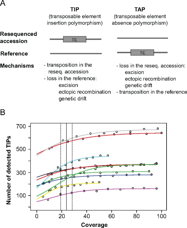
—Coverage down-sampling analysis. (A) Schematic representation of a transposable element insertion polymorphism (TIP) and a transposable element absence polymorphism (TAP). (B) Sampling curves for ten accessions (different colors). Each point along the different lines represents a downsampled data set. The vertical line at x=24 indicates the coverage at which on average 95% of the maximally detectable variants were recovered. The dashed lines show the standard error. Because the downsampling analysis yielded nearly identical results for TIPs and TAPs (x=25±3.4), we here only present the TIP analysis.

Read coverage is an important limiting factor for TE detection algorithms (Stewart et al. 2011; Cridland et al. 2013). While the problem of false positives can be addressed by choosing appropriate filtering criteria (see Material and Methods), false negatives due to low coverage require a different approach. Although coverage was on average 74-fold for the 53 accessions analyzed here, it varied from 8- to 130-fold and also differed between genetic clusters. To evaluate whether these differences in coverage affect the ability of TEMP to detect TE variants, we artificially downsampled the coverage of ten accessions and ran TEMP with the subsets thus obtained.

The resulting sampling curves show that the relationship between coverage and number of detected TE variants follows a logistic model (fig. 4B). On average, a coverage of 24 allows to recover 95% of the TIPs predicted to exist by a logistic growth model (standard error = 4.9), and a coverage of 25 to recover 95% of the TAPs (se = 3.4). As only three accessions analyzed here have a coverage lower than 25 (BdTR8i, Kah-1 and Bd21-3), we concluded that false negatives should not excessively bias our results. In addition, the large nearly horizontal sections of the logistic curves in the figure imply that comparatively high coverages should not create false positives: About the same number of TIPs and TAPs are detected with a coverage of 50 as with a coverage of 100. These results are in line with the simulation study in the original publication of the program (Zhuang et al. 2014), which found that 20-fold coverage allows detecting 95 of the presence polymorphisms, with false discovery rates below 5%.

As an additional control for the reliability of TEMP, the program was also run with paired-end reads from the reference accession Bd21. In this case, because reference reads are mapped against the reference genome, no TE polymorphism should be identified. Indeed, only one TIP and nine TAPs were detected for Bd21, which has a median coverage of 135, thus confirming the low false discovery rate of our method. It also confirms that repetitive regions in the reference genome are well assembled, as otherwise we would expect TEMP to identify collapsed repeats as nonreference insertions and to produce many more false positives. Overall, TEMP thus performs an accurate annotation of TE polymorphisms, its greatest weakness being a high number of false negatives at low coverage which our data, with the exception of three accessions, largely exceed.

TAPs Reflect Active Excision and Genetic Drift

Transposable element absence polymorphisms (TAPs) typically occur at low frequencies: reference TEs are usually absent in only few accessions and therefore most likely shared among the majority of accessions (fig. 5). There is considerable heterogeneity, however, in the frequency spectra of TAPs, not only among the three genetic clusters of B. distachyon, but also between the two different TE classes.

Fig. 5.

—Frequency spectra of TIPs and TAPs. Frequency spectra of TIPs and TAPs in the three genetic clusters. Crosses represent the frequencies of derived nongenic SNPs. Within each plot the number of detected variants is shown as n=number of retrotransposons/number of DNA transposons.

For the 419 absences of reference DNA transposons, a skew toward rare alleles is evident in all three genetic clusters. While a TAP can be due to a recent insertion in the reference accession, the fact that most TAPs only occur in single or few accessions suggests that those elements were once present in these accessions but have been subsequently lost. The punctual loss of a DNA transposon can be straightforwardly explained because these elements can excise from their original insertion site (Wicker et al. 2007). As evidence for this mechanism, we found a strong correlation at the family level between the number of TIPs and TAPs of DNA transposons (R² = 0.77, P-value < 1e-9). This indicates that, following the logic of cut-and-paste transposition, excised DNA transposons detected in the absence analysis have resulted in new insertions which were picked up in the insertion analysis. Most reference DNA transposons thus seem to be older insertions shared among accessions through common descent, while some of these shared TEs got deleted in single or only few accessions through direct excision.

The frequency spectra of retrotransposon TAPs are more complicated. There are large differences between the three genetic clusters of B. distachyon: most strikingly, 184 reference retrotransposons are absent from all the western accessions, while such an increase of high-frequency TAPs is not observed in the other clusters (fig. 5). These 184 TAPs were also detected in the eastern and the relict cluster, although at intermediate frequencies. Therefore, as they display evidence of standing variation, the most parsimonious explanation for their absence in the western accessions is that these 184 reference insertions were lost by genetic drift in the common ancestor of the western accessions, presumably during the severe bottleneck suffered by the ancestral western population (fig. 3). Further support for the explanation that these elements have been lost through drift and not deletion comes from the observation that all of the 100 TAPs we checked manually in a genome browser appear as precise absences of the whole element. Since deletions of retrotransposons typically occur through LTR-LTR recombination and leave behind solo LTRs, deletion events are unlikely to be responsible for the reference TEs missing in the western cluster.

Indeed, if we ignore the spectrum for the relicts which is based on a low number of individuals, the retrotransposon TAP spectra are close to the neutral expectation based on nongenic SNPs: in the western cluster, the frequency distributions of nongenic SNPs and retrotransposon TAPs are highly similar (P = 0.95, Kolmogorov–Smirnov test), while in the east they are marginally different (P = 0.04) due to a slightly increased number of high-frequency TAPs. These patterns contrast with the results for the DNA transposon TAPs whose spectra are strongly shifted toward low frequency alleles in both clusters (P < 0.0001). Overall, our results show that the frequency distributions of retrotransposon TAPs largely reflect the effects of genetic drift, while the predominance of low-frequency DNA transposon TAPs is most likely due to active excision events. Because TAPs thus reflect different molecular and evolutionary mechanisms and, more importantly, because our primary focus in this study is TE activity, we concentrated on the 3,627 TIPs for the rest of the analysis.

TIPs Are Predominantly Lineage-Specific and Indicate Ongoing TE Activity

Among the 3,627 TIPs we identified, the majority occur at low frequencies. Indeed, 1,471 of the 3,232 retrotransposon TIPs and 149 of the 395 DNA transposon TIPs were private to a single accession (fig. 5). Compared to the observed frequencies of derived SNPs in noncoding regions, which show a U-shaped distribution, low-frequency TIPs are highly overrepresented, while fixed TIPs are much less common than fixed SNPs in all clusters.

U-shaped allele frequency distributions can result from strong bottlenecks and further be shifted to high frequency alleles through selective sweeps (Caicedo et al. 2007). The observed spectra for SNPs are thus consistent with our demographic analysis, which showed that ancestral populations of the studied accessions decreased in size during the Quaternary glaciations (fig. 3). The proportion of fixed derived mutations is indeed highest in the western cluster, which confirms that the ancestral western lineage went through a more severe bottleneck than the other lineages.

The frequencies of TIPs are strikingly different. Similar to what has been found in other organisms (Barrón et al. 2014; Ruggiero et al. 2017; Lai et al. 2017), we observe a strong skew toward singleton TIPs and very few fixed TIPs within genetic clusters (fig. 5). One implication of this pattern is that most TIPs are the result of activity in the studied lineages and not ancestral polymorphisms which have been lost in the reference lineage, because old TIPs due to the latter mechanism are expected to segregate at intermediate to high frequencies (Slatkin and Rannala 2000; Kofler et al. 2012). Ongoing activity in expanding populations could contribute to the skew toward rare alleles and explain why the western accessions, which originate from a relatively small geographic area and descend from a bottlenecked lineage, share so few fixed TE polymorphisms (fig. 5). The strong differences, however, between the SNP and TIPs frequency spectra suggest that demographic processes alone cannot explain the predominance of rare TIPs. Two additional factors could contribute to the skew toward rare TIPs: recent bursts of transposition and purifying selection against TEs. We investigate these two processes in the following sections.

Homogeneous TE Family Activity Indicates Conserved Regulatory Mechanisms

The family level is the focal unit in TE biology. Family members are related by common descent from a TE “mother” sequence; they have a common molecular structure and behavior and can be thought of as the “species” in the genome ecosystem (Le Rouzic et al. 2007). As a rule of thumb, two TE sequences are considered as members of the same family when they have 80% sequence identity across at least 80% of the nucleotides (Wicker et al. 2007).

Overall, we found 84 TE families with traces of activity in at least one accession (fig. 6A), ten of them being responsible for 85% of the observed TIPs (fig. 6B;supplementary table S4, Supplementary Material online). Among these ten particularly active families, five are Copia retrotransposons (RLC_BdisC030, RLC_BdisC022, RLC_BdisC026, RLC_BdisC024 and RLC_BdisC010; 55% of all TIPs), four Gypsy retrotransposons (RLG_BdisC152_B, RLG_BdisC004, RLG_BdisC102, RLG_BdisC011; 25% of all TIPs), and one is a Stowaway DNA transposon (DTT_BdisStowawayN; 5% of all TIPs). In some accessions, the most active families account for more than 100 TIPs (fig. 6B). While substantial, these numbers are orders of magnitude below the number of new insertions reported from transpositional bursts in other plant species, during which single TE families can give rise to thousands of new insertions and greatly inflate genome size (Hawkins et al. 2006; Piegu et al. 2006; Tenaillon et al. 2011; Lu et al. 2012). Our results thus confirm the picture of B. distachyon as a species in which TEs show ongoing activity but did not experience massive bursts in the recent past (El Baidouri and Panaud 2013; International Brachypodium Initiative 2010).

Fig. 6.

—TE family activity. (A) Box-plot representing the number of new insertions per TE family across genomes. Only the first 30 out of the 85 TE families with traces of activity are displayed. (B) Number of new insertions identified in each accession for the ten most active TE families. For both panels, the naming of the TE families follows the three-letter convention of Wicker et al. (2007): RLC are Copia LTR retrotransposons, RLG Gypsy LTR retrotransposons, DTT Stowaway DNA transposons, DTC CACTA DNA transposons, and DTH PIF-Harbinger DNA transposons. The three-letter code is followed by the actual family name.

Interestingly, we identified more TIPs in relict accessions than in the others, and more TIPs in western than in eastern accessions (fig. 6B). After correcting for phylogenetic relatedness, however, these differences are not significant anymore (phylogenetic GLS, P > 0.6), suggesting that the western and the relict accessions harbor more TIPs simply because they are more distantly related to the Iraqi reference accession and, while they diverged, accumulated more TIPs than accessions from the eastern cluster. As support of this hypothesis, we found a strong correlation between genetic distance matrices calculated from SNPs and TIPs (Mantel r = 0.8, P < 0.001). This indicates that the number of TIPs we identified is largely associated to genetic distances between accessions and suggests that the general level of TE activity was similar through time in the three studied clusters.

While the number of TIPs varies greatly from one accession to another (fig. 6B), the proportional contribution of each family to TE polymorphisms is largely homogeneous and not significantly different across accessions and genetic clusters (multivariate ANOVA, P = 0.25, fig. 6B). This contrasts with what is observed in A. thaliana (Quadrana et al. 2016) or D. melanogaster (Kofler et al. 2015), where the contribution of individual TE families to mobilome composition can vary significantly between individuals and local populations.

A first possible explanation for this pattern is that the activity level of a family depends on the number of functional copies present in the ancestral genome of B. distachyon. To test this hypothesis, we used the number of full-length elements shared by the 53 genomes as a proxy for the number of functional TE copies in the ancestral genome. This set of shared elements was obtained by assuming that full-length reference insertions that were not detected as absent in any accession (supplementary table S3, Supplementary Material online) are shared by all accessions. In this way, we find that 95 families, including the ten families showing high activity, had full-length copies in the ancestral genome. However, there was no correlation (P = 0.4), neither positive nor negative, between the number of full-length elements present in the ancestral genome and the number of TIPs at the family level. Our results therefore indicate that the overall uniformity of transpositional activity across accessions is not a result of the number of putative functional TE copies inherited from the common ancestor.

Taken together, the similar transposition rates among populations and the homogeneity of family activity indicate that TE activity in B. distachyon is remarkably constant, at least over the microevolutionary timescale considered here. In the past decade, studies reporting transpositional bursts have increasingly cast doubt on formal models of TE dynamics which assume a constant transposition rate (Charlesworth and Charlesworth 1983; Blumenstiel et al. 2014). According to nonequilibrium models (e.g. Rey et al. 2016), TE dynamics are characterized by cycles of environment-induced TE proliferation and subsequent recovery of TE silencing as increasing copy numbers enhance the RNA-directed postranscriptional and epigenetic silencing of TEs (reviewed in Lisch 2009). A prediction following from these models is that diverging lineages will quickly evolve different TE landscapes because the triggers of transpositional bursts, environmental stresses (Rey et al. 2016) and horizontal transfers (El Baidouri et al. 2014), are local events.

Our results disagree with this prediction and suggest that equilibrium models might apply in B. distachyon. In this species, the proliferation of single TE families appears to be not the result of environmental induction, but of regulatory mechanisms which are conserved across populations and allow a low-level activity of certain families. It is therefore highly unlikely that the abundance of rare TIPs described above is due to recent bursts of transposition. Interestingly, a recent analysis of 7 of the 53 accessions used here found no clear evidence for increased DNA methylation around TIPs (Eichten et al. 2016), suggesting that TE silencing is relaxed in B. distachyon. Again, this contrasts with what is observed in A. thaliana, where a clear association is found between TIPs and DNA methylation levels (Stuart et al. 2016). Understanding how TE silencing works in B. distachyon, for example whether TE self-regulation (Charlesworth and Langley 1986) might play a role, now requires further studies investigating the role of siRNAs and methylation in suppressing TE activity.

The Underrepresentation of TIPs in Genic Regions Suggests Purifying Selection against TE Insertions

Since neither demographic history nor transpositional bursts can by themselves account for the predominance of private TIPs, purifying selection might play an important role in causing this skew. In a small genome like the one of B. distachyon, which consists to 38% of genes (International Brachypodium Initiative 2010), a new TE insertion is indeed likely to be deleterious, either by directly disrupting gene function (Sigman and Slotkin 2016) or by causing ectopic recombination events (Petrov et al. 2003).

In accordance with this expectation, both retrotransposons and DNA transposons are underrepresented in exons and overrepresented in intergenic regions relative to the expectations under a random insertion model (table 1). While this is true for all TEs, the different TE superfamilies vary in the strength of this bias and their frequency in other genomic niches (supplementary table S5, Supplementary Material online). Gypsy, Copia, and CACTA elements—all TEs which are relatively large when present as autonomous full-length copies, with consensus lengths ranging from 6,000 (Copia) to almost 12,000 bp (Gypsy)—are rare around and in genes, though this bias is slightly less strong for Copia elements. PIF-Harbinger and Tc1-Mariner DNA transposons, on the other hand, which have consensus lengths of 1,700 and 150 bp, are underrepresented in exons, but more common in the 2 kb neighborhood of genes and in introns, respectively, than expected by chance. At the family level, we observe a positive linear relationship between TE consensus length and the median distance of TIPs to genes (R² = 0.57, P < 0.001, supplementary fig. S1, Supplementary Material online). The distance from a gene scales with the expected length of the TE divided by two: TEs being 2,000 bp longer are on average 1,000 bp further away from a gene.

Table 1.

Genomic Context Analysis

Category	Proportion in Genome	Retrotransposons				DNA Transposons
		Number of TIPs (%)	Observed/Expecteda	P-valueb	Number of TIPs (%)		Observed/Expecteda	P-valueb
Intergenic	25.2	2226 (68.9)	2.73	<0.001	163 (41.3)		1.63	<0.001
Within 2 kb	37.1	760 (23.5)	0.63	<0.001	154 (39)		1.05	0.54
Intron	12.9	107 (3.3)	0.26	<0.001	63 (15.9)		1.24	0.09
Exon	19.2	115 (3.6)	0.15	<0.001	3 (0.8)		0.50	<0.001
5′ UTR	2.1	10 (0.3)	0.12	<0.001	4 (1)		0.57	0.16
3′ UTR	3.6	14 (0.4)	0.19	<0.001	8 (2)		0.04	0.11

^aRatio of observed versus expected number of TIPs in the category. Expected numbers are obtained under a random insertion model which assumes that the probability of inserting into a category is proportional to the genome-wide number of base pairs falling into this category.

^bPoisson test of the random insertion model with λ = exp.

Clearly the size of a TE affects where in the genome it can insert without causing too much harm. In D. melanogaster, the strength of selection against a TE family increases with copy number and element length, which indicates that a homology-based mechanism like ectopic recombination or changes in the chromatin state mediate the deleterious effects of TE insertions (Petrov 2003). It is doubtful, however, whether such a mechanism could play a similarly important role in a selfing organism like B. distachyon, in which homozygosity is high and the effective recombination rate reduced (Wright et al. 2008). In A. thaliana and C. elegans, two selfing organisms, TEs seem to be mainly selected against because of their effect on gene expression rather than because they provoke ectopic recombination events (Wright et al. 2003; Pereira 2004; Hollister and Gaut 2009). Also in this scenario larger TEs are more deleterious than smaller TEs: they are more frequently methylated and therefore more disruptive for the regulatory landscape (Hollister and Gaut 2009). Both models of purifying selection against TEs are thus consistent with our findings, but negative effects on gene expression seem a priori more likely because of the selfing nature of B. distachyon. Altogether, the combined evidence of the scarcity of TEs near genes and their low population frequencies strongly suggests that purifying selection does play an important role in shaping the TE distribution in B. distachyon.

TIPs in Genic Regions Might Contribute to Functional Divergence

Although TIPs are generally less frequent in and around genes than expected by chance, about one third of them occur in genic regions. On average, a relict accession harbors 174 TIPs in genic regions (standard error 19.3), a western accession 134 (3.1), and an eastern accession 67 (4.5). Overall 1,240 genes might be influenced by a new TE insertion (supplementary table S6, Supplementary Material online). As expected from the general skew toward low-frequency alleles, a large proportion of these TIPs are lineage-specific polymorphisms (42%). A substantial amount of the genetic variation caused by TEs does thus not occur in intergenic DNA, but within and especially in the vicinity of genes where it could affect gene expression and host phenotypes. Considering that the genome of B. distachyon is only 272 Mb long and consists, according to the reference annotation, to 38% of genes, it is clear that genic regions are likely to be affected by TE activity. While the relatively high number of TIPs in genic regions is therefore not surprising, it is intriguing that the set of potentially affected genes largely differs from individual to individual. Considering the mutagenic properties of TEs on nearby genes, TEs might thus generate significant functional changes among and within populations of B. distachyon.

Conclusion

Although TEs are key drivers of genome evolution, their role in the evolution of natural populations remains far from clear, especially in plants. Describing TE polymorphisms constitutes the first, necessary step toward illuminating the role of TEs in microevolution. In this study, we show that TE activity is ongoing in B. distachyon and has generated dozens to hundreds insertions in natural accessions. Despite what appears to be a turbulent demographic past, with bottlenecks and recent range expansions shaping genetic diversity in the studied populations, TE family activity seems remarkably homogeneous across the species range. TEs can thus be “well-behaved” even in nonequilibrium populations, which indicates that conserved regulatory mechanisms rather than stress-induced activity are driving TE dynamics in this species. The abundance of rare alleles, together with the underrepresentation of TE variants in genic regions, points to a dominant role of purifying selection in shaping the TE landscape of B. distachyon. We have not undertaken the challenging task of searching for TE insertions which do not correspond to this general pattern but are instead beneficial for the host and under positive selection. The observation, however, that each accession analyzed here carries its own specific set of TIPs in genic regions suggests that TEs might generate significant functional variation among individuals and, eventually, contribute to adaptation.

Data Deposition

Raw sequencing data can be accessed over the JGI Genomes Online Database (GOLD), study ID Gs0033763. The GOLD biosample IDs are listed in supplementary table S1, Supplementary Material online.

Supplementary Material

Supplementary data are available at Genome Biology and Evolution online.

Author Contributions

S.P.G. and J.P.V. generated the raw data. A.R., C.S., and T.W. designed the study. C.S. and A.R. analyzed data. C.S. and A.R. wrote the article.

Literature Cited

- 1001 Genomes Consortium 2016. 1,135 Genomes reveal the global pattern of polymorphism in Arabidopsis thaliana. Cell 166:481–491. [DOI] [PMC free article] [PubMed] [Google Scholar]
- Abascal F. 2016. Extreme genomic erosion after recurrent demographic bottlenecks in the highly endangered Iberian lynx. Genome Biol. 171:251..http://dx.doi.org/10.1186/s13059-016-1090-1 [DOI] [PMC free article] [PubMed] [Google Scholar]
- Alexander DH, Novembre J, Lang K.. 2009. Fast model-based estimation of ancestry in unrelated individuals. Genome Res. 199:1655–1664.http://dx.doi.org/10.1101/gr.094052.109 [DOI] [PMC free article] [PubMed] [Google Scholar]
- Barrón MG, Fiston-Lavier A-S, Petrov DA, González J.. 2014. Population genomics of transposable elements in Drosophila melanogaster. Annu Rev Genet. 48:561–581. [DOI] [PubMed] [Google Scholar]
- Bhattacharyya MK, Smith AM, Ellis THN, Hedley C, Martin C.. 1990. The wrinkled-seed character of pea described by Mendel is caused by a transposon-like insertion in a gene encoding starch-branching enzyme. Cell 601:115–122. [DOI] [PubMed] [Google Scholar]
- Blumenstiel JP, Chen X, He M, Bergman CM.. 2014. An age-of-allele test of neutrality for transposable element insertions. Genetics 1962:523–538.http://dx.doi.org/10.1534/genetics.113.158147 [DOI] [PMC free article] [PubMed] [Google Scholar]
- Bonchev G, Parisod C.. 2013. Transposable elements and microevolutionary changes in natural populations. Mol Ecol Resour. 135:765–775.http://dx.doi.org/10.1111/1755-0998.12133 [DOI] [PubMed] [Google Scholar]
- Brutnell TP, Bennetzen JL, Vogel JP.. 2015. Brachypodium distachyon and Setaria viridis: model genetic systems for the grasses. Annu Rev Plant Biol. 66:465–485.http://dx.doi.org/10.1146/annurev-arplant-042811-105528 [DOI] [PubMed] [Google Scholar]
- Burt A, Trivers R.. 2006. Genes in conflict. Cambridge, USA: Harvard University Press. [Google Scholar]
- Caicedo AL, et al. 2007. Genome-wide patterns of nucleotide polymorphism in domesticated rice. PLoS Genet. 39:1745–1756. [DOI] [PMC free article] [PubMed] [Google Scholar]
- Casacuberta E, González J.. 2013. The impact of transposable elements in environmental adaptation. Mol Ecol. 226:1503–1517. [DOI] [PubMed] [Google Scholar]
- Charlesworth B, Charlesworth D.. 1983. The population dynamics of transposable elements. Genet Res. 4201:1–27.http://dx.doi.org/10.1017/S0016672300021455 [Google Scholar]
- Charlesworth B, Langley CH.. 1986. The evolution of self-regulated transposition of transposable elements. Genetics 1122:359–383. [DOI] [PMC free article] [PubMed] [Google Scholar]
- Cridland JM, Macdonald SJ, Long AD, Thornton KR.. 2013. Abundance and distribution of transposable elements in two Drosophila QTL mapping resources. Mol Biol Evol. 3010:2311–2327. [DOI] [PMC free article] [PubMed] [Google Scholar]
- Danecek P, et al. 2011. The variant call format and VCFtools. Bioinformatics 2715:2156–2158.http://dx.doi.org/10.1093/bioinformatics/btr330 [DOI] [PMC free article] [PubMed] [Google Scholar]
- Dell'Acqua M, Zuccolo A, Tuna M, Gianfranceschi L, Pè ME.. 2014. Targeting environmental adaptation in the monocot model Brachypodium distachyon: a multi-faceted approach. BMC Genomics 15:801.. [DOI] [PMC free article] [PubMed] [Google Scholar]
- Dray S, Dufour A-B.. 2007. The ade4 Package: implementing the duality diagram for ecologists. J Stat Softw. 224:1–20. [Google Scholar]
- Eichten SR, Stuart T, Srivastava A, Lister R, Borevitz JO.. 2016. DNA methylation profiles of diverse Brachypodium distachyon align with underlying genetic diversity. Genome Res. 2611:1520–1531. [DOI] [PMC free article] [PubMed] [Google Scholar]
- El Baidouri M, et al. 2014. Widespread and frequent horizontal transfers of transposable elements in plants. Genome Res. 245:831–838.http://dx.doi.org/10.1101/gr.164400.113 [DOI] [PMC free article] [PubMed] [Google Scholar]
- El Baidouri M, Panaud O.. 2013. Comparative genomic paleontology across plant kingdom reveals the dynamics of TE-driven genome evolution. Genome Biol Evol. 55:954–965.http://dx.doi.org/10.1093/gbe/evt025 [DOI] [PMC free article] [PubMed] [Google Scholar]
- Felsenstein J. 1985. Phylogenies and the comparative method. Am Nat. 1251:1–15. [Google Scholar]
- Feschotte C. 2008. Transposable elements and the evolution of regulatory networks. Nat Rev Genet. 95:397–405.http://dx.doi.org/10.1038/nrg2337 [DOI] [PMC free article] [PubMed] [Google Scholar]
- Garrison E, Marth G.. 2012. Haplotype-based variant detection from short-read sequencing. arXiv:1207.3907.
- González J, Karasov TL, Messer PW, Petrov DA.. 2010. Genome-wide patterns of adaptation to temperate environments associated with transposable elements in Drosophila. PLOS Genet. 64:e1000905.. [DOI] [PMC free article] [PubMed] [Google Scholar]
- González J, et al. 2008. High rate of recent transposable element-induced adaptation in Drosophila melanogaster. PLoS Biol. 610:2109–2129. [DOI] [PMC free article] [PubMed] [Google Scholar]
- Gordon SP, et al. 2017. Extensive gene content variation in the Brachypodium distachyon pan-genome correlates with population structure. Nat Comm. 8:2184. [DOI] [PMC free article] [PubMed]
- Hampe A, Jump AS.. 2011. Climate relicts: past, present, future. Annu Rev Ecol Evol Syst. 421:313–333.http://dx.doi.org/10.1146/annurev-ecolsys-102710-145015 [Google Scholar]
- Hawkins JS, et al. 2006. Differential lineage-specific amplification of transposable elements is responsible for genome size variation in Gossypium. Genome Res. 1610:1252–1261.http://dx.doi.org/10.1101/gr.5282906 [DOI] [PMC free article] [PubMed] [Google Scholar]
- Hollister JD, Gaut BS.. 2009. Epigenetic silencing of transposable elements: a trade-off between reduced transposition and deleterious effects on neighboring gene expression. Genome Res. 198:1419–1428.http://dx.doi.org/10.1101/gr.091678.109 [DOI] [PMC free article] [PubMed] [Google Scholar]
- Hudson RR, Boos DD, Kaplan NL.. 1992. A statistical test for detecting geographic subdivision. Mol Biol Evol. 91:138–151. [DOI] [PubMed] [Google Scholar]
- International Brachypodium Initiative 2010. Genome sequencing and analysis of the model grass Brachypodium distachyon. Nature 463:763–768. [DOI] [PubMed] [Google Scholar]
- Kofler R, Betancourt AJ, Schlötterer C.. 2012. Sequencing of pooled DNA samples (Pool-Seq) uncovers complex dynamics of transposable element insertions in Drosophila melanogaster. PLoS Genet. 81:e1002487.. [DOI] [PMC free article] [PubMed] [Google Scholar]
- Kofler R, Nolte V, Schlötterer C.. 2015. Tempo and mode of transposable element activity in Drosophila. PLOS Genet. 117:e1005406.. [DOI] [PMC free article] [PubMed] [Google Scholar]
- Lai X, et al. 2017. Genome-wide characterization of non-reference transposable element insertion polymorphisms reveals genetic diversity in tropical and temperate maize. BMC Genomics 181:702.http://dx.doi.org/10.1186/s12864-017-4103-x [DOI] [PMC free article] [PubMed] [Google Scholar]
- Lee C, et al. 2017. On the post-glacial spread of human commensal Arabidopsis thaliana. Nat. Commun. 8:14458. [DOI] [PMC free article] [PubMed] [Google Scholar]
- Lee T-H, Guo H, Wang X, Kim C, Paterson AH.. 2014. SNPhylo: a pipeline to construct a phylogenetic tree from huge SNP data. BMC Genomics 15:162.. [DOI] [PMC free article] [PubMed] [Google Scholar]
- Li H. 2013. Aligning sequence reads, clone sequences and assembly contigs with BWA-MEM. arXiv:1303.3997.
- Lisch D. 2009. Epigenetic regulation of transposable elements in plants. Annu Rev Plant Biol. 60:43–66.http://dx.doi.org/10.1146/annurev.arplant.59.032607.092744 [DOI] [PubMed] [Google Scholar]
- Lisch D. 2013. How important are transposons for plant evolution? Nat Rev Genet. 141:49–61. [DOI] [PubMed] [Google Scholar]
- Lockton S, Ross-Ibarra J, Gaut BS.. 2008. Demography and weak selection drive patterns of transposable element diversity in natural populations of Arabidopsis lyrata. Proc Natl Acad Sci USA. 10537:13965–13970. [DOI] [PMC free article] [PubMed] [Google Scholar]
- Lu C, et al. 2012. Miniature inverted-repeat transposable elements (MITEs) have been accumulated through amplification bursts and play important roles in gene expression and species diversity in Oryza sativa. Mol Biol Evol. 293:1005–1017.http://dx.doi.org/10.1093/molbev/msr282 [DOI] [PMC free article] [PubMed] [Google Scholar]
- Lynch M. 2007. The origins of genome architecture. Sinauer Associates. [Google Scholar]
- Lynch M, et al. 2016. Genetic drift, selection and the evolution of the mutation rate. Nat Rev Genet. 1711:704–714.http://dx.doi.org/10.1038/nrg.2016.104 [DOI] [PubMed] [Google Scholar]
- Makarevitch I, et al. 2015. Transposable elements contribute to activation of maize genes in response to abiotic stress. PLoS Genet. 111:e1004915. [DOI] [PMC free article] [PubMed] [Google Scholar]
- Mayr E. 1942. Systematics and the origin of species. New York: Columbia University Press. [Google Scholar]
- Mazet O, Rodríguez W, Grusea S, Boitard S, Chikhi L.. 2016. On the importance of being structured: instantaneous coalescence rates and human evolution—lessons for ancestral population size inference? Heredity 1164:362–371. [DOI] [PMC free article] [PubMed] [Google Scholar]
- Merenciano M, et al. 2016. Multiple independent retroelement insertions in the promoter of a stress response gene have variable molecular and functional effects in Drosophila. PLoS Genet. 128:e1006249. [DOI] [PMC free article] [PubMed] [Google Scholar]
- Morgulis A, Gertz EM, Schäffer AA, Agarwala R.. 2006. A fast and symmetric DUST implementation to mask low-complexity DNA sequences. J Comput Biol. 135:1028–1040. [DOI] [PubMed] [Google Scholar]
- Nieto Feliner G. 2014. Patterns and processes in plant phylogeography in the Mediterranean Basin. A review. Perspect Plant Ecol Evol Syst. 165:265–278.http://dx.doi.org/10.1016/j.ppees.2014.07.002 [Google Scholar]
- Oksanen J, et al. 2017. vegan: Community Ecology Package. R package version 2.4-4. https://CRAN.R-project.org/package=vegan.
- Otto TD, Dillon GP, Degrave WS, Berriman M.. 2011. RATT: rapid annotation transfer tool. Nucleic Acids Res. 399:1–7. [DOI] [PMC free article] [PubMed] [Google Scholar]
- Pannell JR. 2015. Evolution of the mating system in colonizing plants. Mol Ecol. 249:2018–2037.http://dx.doi.org/10.1111/mec.13087 [DOI] [PubMed] [Google Scholar]
- Pereira V. 2004. Insertion bias and purifying selection of retrotransposons in the Arabidopsis thaliana genome. Genome Biol. 510:R79.. [DOI] [PMC free article] [PubMed] [Google Scholar]
- Petrov DA, Aminetzach YT, Davis JC, Bensasson D, Hirsh AE.. 2003. Size matters: non-LTR retrotransposable elements and ectopic recombination in Drosophila. Mol Biol Evol. 206:880–892. [DOI] [PubMed] [Google Scholar]
- Pfeifer B, Wittelsbürger U, Ramos-Onsins SE, Lercher MJ.. 2014. PopGenome: an efficient Swiss army knife for population genomic analyses in R. Mol Biol Evol. 317:1929–1936. [DOI] [PMC free article] [PubMed] [Google Scholar]
- Piegu B, et al. 2006. Doubling genome size without polyploidization: dynamics of retrotransposition-driven genomic expansions in Oryza australiensis, a wild relative of rice. Genome Res 1610:1262–1269.http://dx.doi.org/10.1101/gr.5290206 [DOI] [PMC free article] [PubMed] [Google Scholar]
- Pinheiro J, Bates D, Debroy S, Sarkar D.. 2017. nlme: Linear and Nonlinear Mixed Effects Models R package version 3.1-131, https://CRAN.R-project.org/package=nlme.
- Purcell S, et al. 2007. PLINK: a tool set for whole-genome association and population-based linkage analyses. Am J Hum Genet. 813:559–575.http://dx.doi.org/10.1086/519795 [DOI] [PMC free article] [PubMed] [Google Scholar]
- Quadrana L, et al. 2016. The Arabidopsis thaliana mobilome and its impact at the species level. eLife 5: e15716. [DOI] [PMC free article] [PubMed] [Google Scholar]
- Rey O, Danchin E, Mirouze M, Loot C, Blanchet S.. 2016. Adaptation to global change: a transposable element—epigenetics perspective. Trends Ecol Evol. 317:514–526. [DOI] [PubMed] [Google Scholar]
- Le Rouzic A, Dupas S, Capy P.. 2007. Genome ecosystem and transposable elements species. Gene 390(1–2):214–220. [DOI] [PubMed] [Google Scholar]
- Ruggiero RP, Bourgeois Y, Boissinot S.. 2017. LINE insertion polymorphisms are abundant but at low frequencies across populations of Anolis carolinensis. Front Genet. 8:1–14. [DOI] [PMC free article] [PubMed] [Google Scholar]
- Sanseverino W, et al. 2015. Transposon insertion, structural variations and SNPs contribute to the evolution of the melon genome. Mol Biol Evol. 3210:2760–2774.http://dx.doi.org/10.1093/molbev/msv152 [DOI] [PubMed] [Google Scholar]
- Schrader L, et al. 2014. Transposable element islands facilitate adaptation to novel environments in an invasive species. Nat. Commun 5:5495.. [DOI] [PMC free article] [PubMed] [Google Scholar]
- Sigman MJ, Slotkin RK.. 2016. The first rule of plant transposable element silencing: location, location, location. Plant Cell 282:304–313.http://dx.doi.org/10.1105/tpc.15.00869 [DOI] [PMC free article] [PubMed] [Google Scholar]
- Slatkin M, Rannala B.. 2000. Estimating allele age. Annu Rev Genomics Hum Genet. 1:225–249.http://dx.doi.org/10.1146/annurev.genom.1.1.225 [DOI] [PubMed] [Google Scholar]
- Slotkin RK, Martienssen R.. 2007. Transposable elements and the epigenetic regulation of the genome. Nat Rev Genet. 84:272–285.http://dx.doi.org/10.1038/nrg2072 [DOI] [PubMed] [Google Scholar]
- Stebbins GL. 1957. Self fertilization and population variability in the higher plants. Am Nat. 91861:337–354.http://dx.doi.org/10.1086/281999 [Google Scholar]
- Stewart C, et al. 2011. A comprehensive map of mobile element insertion polymorphisms in humans. PLoS Genet. 78:e1002236. [DOI] [PMC free article] [PubMed] [Google Scholar]
- Stuart T, Eichten S, Cahn J, Borevitz J, Lister R.. 2016. Population scale mapping of transposable element diversity reveals links to gene regulation and epigenomic variation. eLife 5:e20777. [DOI] [PMC free article] [PubMed] [Google Scholar]
- Suzuki R, Shimodaira H.. 2006. Pvclust: an R package for assessing the uncertainty in hierarchical clustering. Bioinformatics 2212:1540–1542.http://dx.doi.org/10.1093/bioinformatics/btl117 [DOI] [PubMed] [Google Scholar]
- Tarasov A, Vilella AJ, Cuppen E, Nijman IJ, Prins P.. 2015. Sambamba: fast processing of NGS alignment formats. Bioinformatics 3112:2032–2034. [DOI] [PMC free article] [PubMed] [Google Scholar]
- Tenaillon MI, Hollister JD, Gaut BS.. 2010. A triptych of the evolution of plant transposable elements. Trends Plant Sci. 158:471–478.http://dx.doi.org/10.1016/j.tplants.2010.05.003 [DOI] [PubMed] [Google Scholar]
- Tenaillon MI, Hufford MB, Gaut BS, Ross-Ibarra J.. 2011. Genome size and transposable element content as determined by high-throughput sequencing in maize and Zea luxurians. Genome Biol Evol. 3:219–229. [DOI] [PMC free article] [PubMed] [Google Scholar]
- Terhorst J, Kamm JA, Song YS.. 2017. Robust and scalable inference of population history from hundreds of unphased whole genomes. Nat Genet. 492:303–309. [DOI] [PMC free article] [PubMed] [Google Scholar]
- Tian Z, et al. 2012. Genome-wide characterization of nonreference transposons reveals evolutionary propensities of transposons in soybean. Plant Cell 2411:4422–4436.http://dx.doi.org/10.1105/tpc.112.103630 [DOI] [PMC free article] [PubMed] [Google Scholar]
- Tyler AL, et al. 2016. Population structure in the model grass Brachypodium distachyon is highly correlated with flowering differences across broad geographic areas. Plant Genome 9. doi:10.3835/plantgenome2015.08.0074. [DOI] [PubMed]
- van’t Hof AE, et al. 2016. The industrial melanism mutation in British peppered moths is a transposable element. Nature 5347605:102–105. [DOI] [PubMed] [Google Scholar]
- Van Buren R, Mockler TC.. 2016. The Brachypodium distachyon reference genome In: Vogel JP, editor. Genetics and genomics of Brachypodium. Berlin, Heidelberg, New York: Springer International Publishing; p. 55–70. [Google Scholar]
- Vitte C, Fustier MA, Alix K, Tenaillon MI.. 2014. The bright side of transposons in crop evolution. Brief Funct Genomics 134:276–295.http://dx.doi.org/10.1093/bfgp/elu002 [DOI] [PubMed] [Google Scholar]
- Vogel JP, et al. 2009. Development of SSR markers and analysis of diversity in Turkish populations of Brachypodium distachyon. BMC Plant Biol. 9:88.. [DOI] [PMC free article] [PubMed] [Google Scholar]
- Wakeley J. 1996. The variance of pairwise nucleotide differences in two populations with migration. Theor Popul Biol. 491:39–57.http://dx.doi.org/10.1006/tpbi.1996.0002 [DOI] [PubMed] [Google Scholar]
- Wei B, et al. 2016. Genome-wide characterization of non-reference transposons in crops suggests non-random insertion. BMC Genomics 17:536.. [DOI] [PMC free article] [PubMed] [Google Scholar]
- Wicker T, et al. 2007. A unified classification system for eukaryotic transposable elements. Nat Rev Genet. 812:973–982.http://dx.doi.org/10.1038/nrg2165 [DOI] [PubMed] [Google Scholar]
- Wilson P, Streich J, Borevitz JO.. 2016. Genome diversity and climate adaptation in Brachypodium In: Vogel JP, editor. Genetics and genomics of Brachypodium. Berlin, Heidelberg, New York: Springer; p. 107–127. [Google Scholar]
- Wright SI, Agrawal N, Bureau TE.. 2003. Effects of recombination rate and gene density on transposable element distributions in Arabidopsis thaliana. Genome Res. 138:1897–1903. [DOI] [PMC free article] [PubMed] [Google Scholar]
- Wright SI, Ness RW, Foxe JP, Barrett SCH.. 2008. Genomic consequences of outcrossing and selfing in plants. Int J Plant Sci. 1691:105–118. [Google Scholar]
- Xiao H, et al. 2008. A retrotransposon-mediated gene duplication underlies morphological variation of tomato fruit. Science 3195869:1527–1530.http://dx.doi.org/10.1126/science.1153040 [DOI] [PubMed] [Google Scholar]
- Zheng X, et al. 2012. A high-performance computing toolset for relatedness and principal component analysis of SNP data. Bioinformatics 2824:3326–3328.http://dx.doi.org/10.1093/bioinformatics/bts606 [DOI] [PMC free article] [PubMed] [Google Scholar]
- Zhuang J, Wang J, Theurkauf W, Weng Z.. 2014. TEMP: a computational method for analyzing transposable element polymorphism in populations. Nucleic Acids Res. 4211:6826–6838.http://dx.doi.org/10.1093/nar/gku323 [DOI] [PMC free article] [PubMed] [Google Scholar]
- Zuur AF, Ieno EN, Walker N, Saveliev AA, Smith GM.. 2009. Mixed effects models and extensions in ecology with R. New York: Springer. [Google Scholar]
Associated Data
This section collects any data citations, data availability statements, or supplementary materials included in this article.