Cooperative and Competitive Interactions Facilitate Stereo Computations in Macaque Primary Visual Cortex

Abstract

Inferring depth from binocular disparities is a difficult problem for the visual system because local features in the left- and right-eye images must be matched correctly to solve this “stereo correspondence problem.” Cortical architecture and computational studies suggest that lateral interactions among neurons could help resolve local uncertainty about disparity encoded in individual neurons by incorporating contextual constraints. We found that correlated activity among pairs of neurons in primary visual cortex depended both on disparity-tuning relationships and the stimuli displayed within the receptive fields of the neurons. Nearby pairs of neurons with distinct disparity tuning exhibited a decrease in spike correlation at competing disparities soon after response onset. Distant neuronal pairs of similar disparity tuning exhibited an increase in spike correlation at mutually preferred disparities. The observed correlated activity and response dynamics suggests that local competitive and distant cooperative interactions improve disparity tuning of individual neurons over time. Such interactions could represent a neural substrate for the principal constraints underlying cooperative stereo algorithms.

Introduction

A fundamental problem of visual inference is that a local piece of incoming visual information is often ambiguous and subject to multiple interpretations. Computational and neurophysiological studies have proposed that contextually constrained interactions among neurons with a variety of receptive field locations and stimulus preferences can facilitate the visual inference process (Marr, 1982; Eckhorn et al., 1988; Gray et al., 1989; Kapadia et al., 1995; Ringach et al., 1997; Ben-Shahar et al., 2003). Interactions among neurons can reduce uncertainty caused by noisy, incomplete, and ambiguous incoming visual signals. Often, uncertainty arises even with perfect visual signals because of multiple potential interpretations of the incoming information.

Local ambiguity is a severe problem when making three-dimensional interpretations of the visual scene. For example, deriving depth information from binocular disparity requires matching features in the left- and right-eye images that correspond to the same point in space. Several models have been proposed to solve this correspondence problem (for review, see Tsai and Victor, 2003). Each model offers solutions to stereopsis problems with specific conditions of computing disparity. Thus far, most neurophysiological research has focused on predictions made by the localized disparity energy model (Ohzawa et al., 1990; DeAngelis et al., 1991; Cumming and DeAngelis, 2001; Prince et al., 2002; Parker, 2007). Only one recent study has examined interactions among disparity-tuned neurons and tested predictions made by more complex computational models of stereo matching (Menz and Freeman, 2003). In that study, Menz and Freeman described a coarse-to-fine spatial scale constraint for local feedforward processing. Here, we examine the spatial organization and constraints for lateral interactions among disparity-tuned neurons. We specifically test predictions made by the subset of models that incorporate one or both of the constraints (Sperling, 1970; Dev, 1975; Nelson, 1975; Marr and Poggio, 1976; Pollard et al., 1985; Prazdny, 1985) used in cooperative stereo algorithms (Marr and Poggio, 1976). Cooperative models of stereo computations are highly adept at solving the correspondence problem for random dot stereograms (RDSs) (Marr and Poggio, 1976). Additionally, cooperative computations of disparity could have much wider implications by explaining several psychophysical phenomena that suggest that disparity information is propagated spatially (Julesz and Chang, 1976; Marr and Poggio, 1979; Collett, 1985; Mitchison and McKee, 1985; Ramachandran and Cavanaugh, 1985; Westheimer, 1986; Stevenson et al., 1991).

We found evidence for both suppressive and facilitative interactions among disparity-tuned neurons. Pairs of neurons with distinct disparity tuning and coexistent receptive fields had reduced spike correlation soon after stimulus onset. At longer delays and greater distance between receptive fields, pairs of neurons had increased spike correlation that was stronger when disparity tuning was more similar. The temporal evolution of disparity tuning was also suggestive of disparity-dependent competitive and cooperative interactions. Although not conclusive, these observations are consistent with the predictions made by the constraints of cooperative models of stereo computations.

Materials and Methods

Physiological preparation.

A detailed description of the physiological preparation for the monkeys used in these experiments can be found in a previous study (Smith et al., 2007). All procedures were approved by the Institutional Animal Care and Use Committee of Carnegie Mellon University and are in accordance with the National Institutes of Health Guide for the Care and Use of Laboratory Animals. In brief, a cranial recording chamber overlying the operculum of V1 and sclera eye coil were implanted in two rhesus monkeys (Macaca mulatta) under full sterile conditions while monkeys were anesthetized by inhalation (1.5% isoflurane).

Recording.

Transdural recordings were made in the chamber with 60 mm tungsten-in-epoxy and tungsten-in-glass microelectrodes (FHC) in the two awake, behaving monkeys. Two to eight microelectrodes were introduced into V1 using custom-made manually driven delron microdrives (A-Z Machining Service). Microdrives were designed to each hold and drive up to four electrodes simultaneously. We attached microdrives to a grid that was inserted into the recording chamber. Electrode configurations were always within a 2 × 4 hole region of the grid with a minimum and maximum potential interelectrode distance of 0.5 and 3.2 mm, respectively (Fig. 1A). Grid spacing was 1 mm, but for some experiments, electrodes were inserted at an angle with respect to other electrodes to allow for even tighter spacing (spacing within cortex was undetermined, but was constrained to 500 μm based on electrode dimensions). Each electrode was permanently attached to the microdrive with cyanoacrylate. Multielectrode microdrives prevented us from advancing all electrodes independently. However, we could advance each microdrive independently. All electrodes were inserted at a similar depth with respect to the grid in which microdrives were attached. However, recordings were potentially in different V1 layers based on the variability in transdural insertion, as well as the curvature of the cortex.

Figure 1.

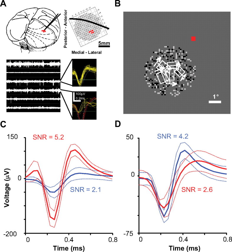
A, B, An example recording session. In this session, we used three dual electrode microdrives in a 2 × 3 configuration (one electrode failed to record neural activity and was disconnected). A, Position of the six-electrode array with respect to the macaque brain and the grid where microdrives were attached within the recording chamber (dashed lines are approximate retinotopic coordinates and solid black line overlaying the grid is approximate location of the lunate sulcus based on several previous recording sessions within this chamber). The bottom plots show filtered neural activity for all channels and samples of triggered and on-line sorted action potentials. B, Receptive field locations (minimum response field) with respect to fixation (red) and DRDS stimulation. C, D, Examples of multiple waveforms (dotted lines are SDs) recorded on the same electrode. C, We typically encountered multiple units that were easily distinguishable (these are waveforms for the competitive example pair of neurons described in the main text). D, The most waveform overlap that was allowed to consider multiple waveforms on the same electrode for cross-correlation analysis.

Connections between electrodes and a Tucker-Davis 16-channel headstage were made with independently shielded micro-coaxial wire (World Precision Instruments). These signals were digitally sampled at 24.4 kHz with a Tucker-Davis 16-channel Medusa preamplifier and bandpass filtered between 2.2 Hz and 7.5 kHz. Digital signals were then processed with a Tucker-Davis RX5 Pentusa base station and Open Explorer software. Each channel was digitally filtered between 300 Hz and 7 kHz and action potentials (22 samples) were triggered by a manually set threshold. Time-window threshold sorting was used for basic on-line receptive field characterization (Fig. 1A,B).

All subsequent analyses were performed on off-line sorted data using principal component analysis (PCA) (Shoham et al., 2003). We used PCA spike sorting to remove any potential artifact and noise, as well as to isolate the most robust single-unit or multiunit waveform. Multiple waveforms were analyzed on the same electrode only if waveform SDs were completely nonoverlapping for at least one of the 22 samples (Fig. 1C,D). Seventeen of the 63 pairs described in the article were recorded on the same electrode. We found the best compromised depth for each microdrive, which produced signal-to-noise ratio values (μ = 2.9 ± 0.1) that were mostly comparable with typical single-unit recordings in more stable paralyzed and anesthetized preparations (Kelly et al., 2007).

Stimulation.

Stimuli were presented to the monkeys on a 21 inch Sony Trinitron cathode ray tube with a 120 Hz refresh rate and mean luminance of 39 cd/m². For basic receptive field characterization, we used two forms of stimulation. First, a white or black bar was manually drifted across the receptive field while the monkey fixated to approximately determine the receptive field center. Then, a white or black bar was automatically drifted across the receptive field at eight different directions (45° increments) at 2°/s for more accurate receptive field plotting, as well as to quantify orientation tuning and direction selectivity. For stereoscopic stimuli, left- and right-eye images were presented in alternating frames using liquid crystal shutter goggles (Stereographics). Dynamic RDSs (DRDSs) were presented for 1 s in a 3.5° aperture with 25% dot density (half-black, half-white; 0.094° size) and random dot patterns were updated at a rate of 12 Hz (Fig. 1B). Thirty different DRDS movies (360 random dot patterns) were presented twice for a total of 60 trials for each of 11 disparities (±0.94, ±0.658, ±0.282, ±0.188, ±0.094, 0°). For three recording sessions (n = 8 neurons), we presented only seven disparities (±0.94, ±0.658, ±0.282, 0°). Stimulus onset was registered with submillisecond precision by recording a digital pulse after a frame reset immediately preceding the start of DRDS presentation.

Cross-correlation analysis.

We used standard cross-correlation methods to measure the dynamics of interactions (Aertsen et al., 1989). First, the probability of joint spike occurrences between two neurons was calculated in 1 ms bins at all possible lag times, all possible times from stimulus onset, and for all disparities presented by averaging counts over 60 trials. Second, the chance probability of joint spike occurrences was determined by taking the outer product of the peristimulus time histograms (PSTHs). This was the expected joint spike occurrences based on the instantaneous average firing probabilities, if the two neurons were independent. The cross-covariance histogram is the difference between joint spike occurrences and chance joint spike occurrences as follows:

The cross-covariance histogram was then normalized by the square root of the product of the two auto-covariance histograms for each neuron to produce a histogram of Pearson's correlation coefficients as follows:

We next extracted all correlation measurements from this normalized cross-covariance histogram (also referred to as the normalized joint poststimulus time histogram).

We first derived the traditional cross-correlation histogram (CCH) by averaging along the principal diagonal. We calculated this CCH with as many spikes as possible because more spikes provide a more reliable estimate of the following: (1) whether or not two neurons interact (correlated spiking responses) at any of the disparities presented and if they interact, (2) the temporal window of that interaction. CCHs were smoothed with a window that was based on the width of the central peak (median, 15 ms; maximum, 40 ms). Next, we calculated the SD of the CCH within a window far from the central peak (±175–375 ms lag time) for each disparity presented. We set a threshold for interacting pairs to be 3 SDs above zero. The CCH had to pass this threshold within ±10 ms of zero lag time for any disparity presented to be included in subsequent analysis. We then also assessed confidence in the CCH peak by examining variance across trials by bootstrapping CCH estimates (Efron and Tibshirani, 1993; Ventura et al., 2005b).

Next, we integrated the area under the central peak in the CCH (half-height, full-width) (Das and Gilbert, 1999; Menz and Freeman, 2003). Correlation cannot be estimated at zero lag time for two neurons recorded on the same electrode (waveforms overlap within the same signal), which creates a large artifact negative peak. This artifact for pairs of neurons recorded on the same electrode was excluded in central peak integration. The integration provided us with the most robust estimate of correlation maximizing the number of spikes included so that we could examine the correlation changes with respect to disparity and time. This represents the total correlation or percentage of spikes from one neuron that co-occurred with spikes in the other neuron within the window of time observed from the CCH independent of changes in firing rate. Positive or negative correlation does not imply one neuron is driving or suppressing another neuron. Positive or negative correlation only suggests that the neuronal pair is connected in some manner that causes the second neuron to spike or not spike whenever the first neuron spikes. To determine whether disparity influenced correlation, we repeated this half-height full-width integration for all disparities. We then used this same half-height full-width integration across time to estimate correlation in 100 ms windows for every 1 ms.

Correlation in trial-to-trial variability can lead to CCH structure with the same temporal precision as the response structure (Brody, 1999). Because the temporal window of neural interaction (CCH peak widths ranged from 3 to 83 ms) that we observed overlapped with the temporal structure of our stimulus (12 Hz), which in turn led to some 12 Hz response modulation, this is an important consideration for our correlation interpretations. Therefore, we carefully tested and provided some correction for the effects of trial-to-trial variability with our correlation estimates. First, we incorporated a correction factor into Equation 2 to account for trial-to-trial changes in the average firing rate (based on the entire stimulus duration). The correction has been mentioned and routinely used in previous studies (Brody, 1999; Gerstein and Kirkland, 2001), but has not been explicitly described until recently (Ventura et al., 2005a). In short, the outer product terms are corrected based on the average firing rate for each neuron for each trial. The PSTH profiles (determined with all trials) are assumed to be stationary so this correction only scales each PSTH for changes in average firing from trial-to-trial as follows:

where n is trial number, N is total trials, θ(n) is average firing rate for trial n, and θ̄ is average firing rate for all trials. This does not correct for all potential sources of variability and is usually referred to as an excitability correction (Brody, 1999; Gerstein and Kirkland, 2001; Ventura et al., 2005a).

Second, we bootstrapped our estimates with respect to trials (Efron and Tibshirani, 1993; Ventura et al., 2005b). For any correlation measurement we reported in the main text, we calculated a raw estimate and then a distribution of 200 estimates using a random selection of 60 trials (allowing repeats). We then subtracted the raw estimate from the mean of this distribution to estimate bias caused by undersampling, which was last subtracted from the raw estimate (final debiased estimate). The 2.5th and 97.5th percentile estimates in the bootstrap distribution were used in the same manner to estimate 95% confidence intervals. We found no noticeable difference in calculations when using larger numbers of bootstrapped estimates.

Finally, we checked for the influence of trial-to-trial stimulus variability. Because we displayed 30 different DRDSs two times, this allowed us to measure correlation using a simpler cross-correlation measurement in which only a single trial was used to estimate chance joint occurrences—the shift predictor corrected CCH (Bair et al., 2001; Kohn and Smith, 2005). Although this technique is noisier and there is also a subtle difference in normalization, we can still compare CCHs using the shift predictor and the normalized cross-covariance histogram because they are nearly equivalent measurements (Aertsen et al., 1989; Bair et al., 2001). With shift predictor estimation of chance joint occurrences, we remove variability caused by the stimulus by shifting (or sometimes called shuffling) trials for each neuron to opposite trials for the exact same DRDS.

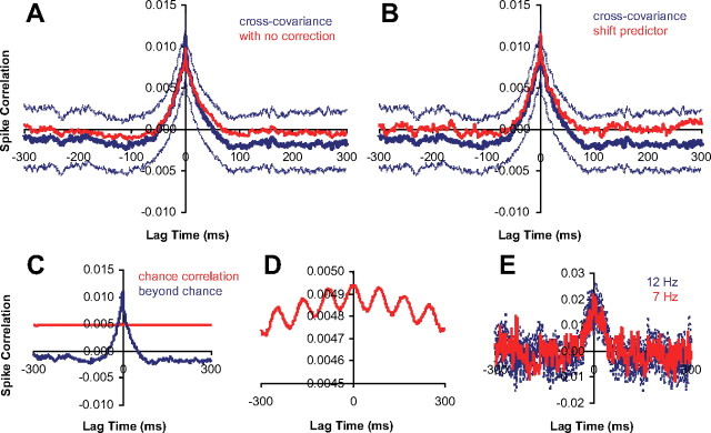
Figure 2A illustrates that we found negligible differences in the region of the CCH in which we focus all of our analyses (near zero lag time) when we included excitability and bootstrap correction to cross-covariance measurements. The excitability correction did not remove the peak, but only shifted the entire CCH to a lower value. The reason for little change in the peak is that the 12 Hz modulation in the stimulus leads to only a moderate 12 Hz response modulation. Equation 3 (excitability correction) only rescales the probability of chance correlation as follows:

Because the chance correlation (Fig. 2C, red) is flat compared with the beyond chance correlation (Fig. 2C, blue), it only shifts the estimated CCH. Although we indeed can see a 12 Hz response modulation in the chance correlation with closer inspection (Fig. 2D), on average, the 12 Hz chance correlation structure is 100 times smaller than the beyond chance central peak correlation structure. Overall, we did notice some 12 Hz oscillation in CCHs, but it was always much smaller than the CCH central peak and only added a small amount of noise to our measurements. As an additional test, we used DRDSs with different modulation rates during some recording sessions. Figure 2E shows the results for a pair of neurons tested with DRDSs at different modulation rates. CCH peak width did not change whether DRDSs were modulated at 12 or 7 Hz. If the CCH peak did arise from trial-to-trial nonstationarity factors, the peak width should have increased from 12 to 7 Hz. Finally, there was also little difference between our cross-covariance estimates and shift-predictor estimates (Fig. 2B), suggesting stimulus variability was also negligible in correlation measurements. Overall, our analysis suggests that trial-to-trial variability and any associated correction were unlikely to have been major factors in our conclusions.

Figure 2.

A, B, Population average of normalized CCHs (n = 63 pairs, centered on their peak). The dotted lines are population average of individual pairs' 95% confidence intervals (n = 60 trials). A, Raw cross-covariance derived CCH (red) versus excitability corrected and bootstrapped CCH (blue). B, Shift-predictor CCH (red) versus excitability corrected and bootstrapped CCH (blue). C, Population average CCH (blue) and chance correlation (red). D, Zoomed-in plot of chance correlation. E, Example CCH for DRDS modulated at 12 or 7 Hz (dashed lines are bootstrapped 95% confidence interval; n = 60 trials).

Eye movement analysis.

Eye movement could have influenced our results and interpretations in two ways. First, binocular stimulation could trigger vergence eye movements that would change the binocular disparity during stimulation. Second, changes in fixation across trials and within trials lead to variability in the relationship of our stimulus and the receptive field of the neuron.

Because we did not record movement for both eyes, we did not measure vergence directly. However, the variation of monocular eye movements within a trial (≪0.1°) (see supplemental Fig. 1, available at www.jneurosci.org as supplemental material), the size of the disparities tested (≥0.094°), and the assumption of some symmetry during vergence suggests that we could still indirectly measure some vergence. Our biggest concern with this analysis was whether or not there was symmetry between left- and right-eye movements during vergence. One reason eye movements would be asymmetric is if the monkeys were trained to avoid vergence based on feedback from data from a single eye. Instead of avoiding vergence, the monkey could develop a strategy of using asymmetric vergence to maintain the position of the single eye within the fixation window. We avoided this scenario because our fixation window was large enough (±0.5°) that vergence movements were allowed even for our largest disparities tested (0.94°). We should note that the monkeys fixated with much greater accuracy than the fixation window allowed (supplemental Fig. 1, available at www.jneurosci.org as supplemental material).

To verify that we could observe vergence based on data from one eye, we measured eye movements (digitally sampled at 976 Hz) during a task in which the monkeys had to fixate on a point that was rendered binocularly at the same depths as the DRDSs used during recordings (supplemental Fig. 1A, available at www.jneurosci.org as supplemental material). The data obtained from this task revealed clear and significant disparity-dependent horizontal eye movements for both monkeys (n = 60 trials; p < 0.0001; one-way ANOVA) that were consistent with vergence movements. The relationship between eye movement and disparity was highly significant when we used mean position, variance of position, or correlation of position with time. For near disparities, the left eye moved horizontally outward (left or uncrossed) (supplemental Fig. 1C,D, available at www.jneurosci.org as supplemental material). For far disparities, the left eye moved horizontally inward (right or crossed) (supplemental Fig. 1G,H, available at www.jneurosci.org as supplemental material). This movement was clearly observed even for the smallest disparities tested during recording (0.094°). And finally, the results in supplemental Figure 1 (available at www.jneurosci.org as supplemental material) support the assumption of symmetry because the mean position of the left eye changed with equal, but opposite, magnitude for near and far disparities (and the magnitude was equal to one-half the disparity presented). To clearly summarize the disparity-dependent vergence movements, we plotted the correlation of horizontal eye positions with time for each disparity tested to show the transition from divergence to convergence (supplemental Fig. 1K,L, available at www.jneurosci.org as supplemental material).

Once we established that we could observe evidence of vergence based on position data from one eye for even the smallest disparities used during recordings, we tested whether or not there was evidence of vergence during DRDS stimulation (supplemental Fig. 1B, available at www.jneurosci.org as supplemental material). When the DRDSs were 4° away from the fixation point, we did not find significant disparity-dependent horizontal eye movements for both monkeys (n = 120 trials; p > 0.05; one-way ANOVA) when we used mean position, variance of position, or correlation of position with time (supplemental Fig. 1, available at www.jneurosci.org as supplemental material, compare the right half with the left half). Across the multiple recording sessions that generated the data for this study, we observed similar nonsignificant results. This was because we made sure that we only recorded from neurons with receptive fields sufficiently far enough from fixation (μ = 4.0 ± 0.1°) so that the stimulus would not induce vergence (supplemental Fig. 2, available at www.jneurosci.org as supplemental material). We also tested for vergence outside of recording sessions for DRDSs that were presented right on top of (or behind) the fixation point, which was displayed at 0° disparity. For only one monkey, we found a weak, but significant disparity-dependent effect that indicated the DRDSs were able to encourage vergence errors for only the smallest disparities presented and only when presented right at fixation (n = 120 trials; p < 0.0001; one-way ANOVA). This was not a problem during recordings because DRDSs were positioned sufficiently far enough away from the fixation point (supplemental Fig. 2, available at www.jneurosci.org as supplemental material).

Our eye movement analysis may have still failed to measure more subtle vergence errors during stimulation because the range of horizontal positions is equal to the smallest disparities tested. These errors could have lead to changes in the neuronal responses in two ways. First, correlation between spike trains could increase and decrease over time in a disparity-dependent manner. If this were the case, we would expect our results to show systematic disparity-dependent changes in spike correlation regardless of the preferred disparity of the neuron. The vergence errors would be independent of the behavior of the neuron and only occur for near and/or far disparities and not for zero disparity DRDS. We did not observe such systematic behavior. Disparity dependence of spike correlation depended explicitly on the preferred disparities of the neurons and we observed similar evidence of cooperative and competitive interactions for all possible combinations of preferred disparities for neuronal pairs. Second, correlation between spike trains could increase at stimulus disparities where the slopes of the two turning curves had the same sign and decrease where the slopes had the opposite sign. We compared the average spike correlation for neuronal pairs for these two conditions and found no significant difference (p = 0.96) (supplemental Fig. 3, available at www.jneurosci.org as supplemental material).

Finally, disparity tuning of individual neurons could change over time. If vergence errors were occurring, disparity tuning would become weaker over time because some or all stimuli would be viewed as 0° disparity as vergence occurred. However, we found the opposite effect: disparity tuning improved over time for neurons with near, far, or zero preferred disparity.

Results

Cooperative algorithms for solving the correspondence problem tend to rely on one or both of the following constraints. The first constraint is termed uniqueness: each location in an image can only be assigned a single disparity solution. This would suggest local competition: a suppressive interaction among neurons that encode different disparities at the same spatial location. The second constraint is termed continuity: depth changes gradually along an object because of the cohesiveness of matter, so a disparity solution at one location is more likely to be correct if the solution for an adjacent location is similar. This would suggest cooperation: a facilitative interaction among neurons that detect the same disparity at different but neighboring locations. Each neuron would in effect reinforce the disparity estimates of its neighbors.

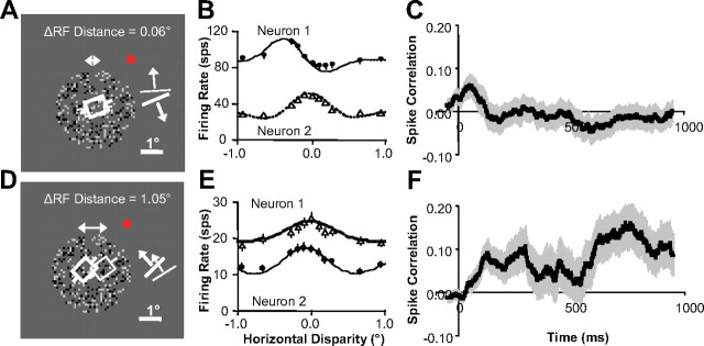
We hypothesized that interactions among a population of visual cortical neurons tuned for a variety of disparities and spatial locations would satisfy the dual constraints of uniqueness and continuity and implement a general depth inference computation. We predicted that two neurons representing the same region (Fig. 3A) of the visual field and preferring distinct disparities (Fig. 3B) would interact competitively. This would lead to negative correlation among spike trains (spike correlation) and a decrease in firing rate over time when nonpreferred disparities are presented. We predicted that two neurons representing neighboring regions of the visual field (Fig. 3D) and favoring similar disparities (Fig. 3E) would interact cooperatively. This would lead to positive spike correlation and an increase in firing rate over time when disparities preferred by both neurons are presented relative to when all other disparities are presented.

Figure 3.

Evidence of competitive and cooperative interaction. A, Neurons with overlapping receptive fields that were presented random dot stereograms (only the image for one eye is shown). The white squares and bars are preferred orientation and direction of motion. The red square is fixation point. B, Disparity tuning for neurons in A. C, Correlation versus time (100 ms sliding windows) for same data shown in B (averaged over all disparities). D, Neurons with neighboring receptive fields. E, Disparity tuning for neurons in D. F, Correlation versus time for same data shown in E (averaged over all disparities). All error bars are trial-to-trial SE (n = 60).

Spike correlation between disparity-tuned neurons

We first examined whether the data matched our computational predictions with respect to spike correlation. To test these predictions across a population of neuronal pairs, we recorded from two to eight microelectrodes inserted in primary visual cortex of two awake, behaving macaques (see Materials and Methods). Since some electrodes recorded the activity of multiple neurons that had discriminable spike waveforms, this technique allowed us to examine responses of up to 10 neurons simultaneously. We recorded from a total of 342 pairs representing combinations of 154 neurons. From this population, 103 neurons (67%) had significant disparity tuning (one-way ANOVA, p < 0.01) and 154 pairs (45%) were composed of two neurons that both had significant disparity tuning. This sample of neuronal pairs provided us with sufficient diversity in both receptive field relationships and preferred disparities to test our predictions.

We presented 1 s DRDSs to monkeys trained to fixate during stimulation. DRDSs were updated with a new set of dot positions at 12 Hz and rendered at 11 different horizontal disparities. We quantified spike correlation between pairs of neurons by cross-correlating spike trains over 60 trials at each of the 11 disparities presented (see Materials and Methods). The CCH over the entire stimulus duration provided us with a function of spike correlation versus the delay between spikes (lag time) for the two neurons. This calculation tells us the probability (beyond chance) of a spike occurring in one neuron whenever a spike occurs in the other neuron at different lag times. We used this CCH to determine whether or not neuronal pairs were interacting for any disparity presented and, if they were, over what window of time. Of 154 pairs of neurons with significant disparity tuning, 63 (41%) had a correlation peak or valley greater than a threshold determined by standard criteria for at least one disparity presented (see Materials and Methods). For each of these 63 pairs of neurons, we integrated the spike correlation under the half-height width of the central CCH peak to examine interactions for these pairs of neurons as a function of disparity-tuning similarity, disparity presented, and time from stimulus onset.

Figure 3C shows that the example pair of neurons predicted to interact competitively had positive spike correlation (averaged over all disparities presented) that decreased soon after response onset resulting in negative spike correlation during stimulation. This negative spike correlation supports our prediction of competition between these neurons. Figure 3F shows that the example pair of neurons predicted to interact cooperatively had zero spike correlation (again, averaged over all disparities presented) that increased soon after response onset resulting in bursts of positive spike correlation during stimulation. This positive spike correlation supports our prediction of cooperation between these neurons.

To summarize how average spike correlation varied with distance and similarity in disparity tuning for each neuronal pair, we measured the distance between receptive field centers, the disparity-tuning similarity (correlation between tuning curves: r_disp), and the average spike correlation over the entire stimulus period (excluding the initial 50 ms before response onset).

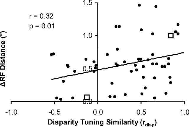
In Figure 4, the distance between receptive fields is plotted versus disparity-tuning similarity for neuronal pairs that had significant average spike correlation. As the distance between receptive fields increased to >1.0° (with this separation, V1 receptive fields have little or no overlap), we only observed spike correlation for neuronal pairs with similar disparity tuning (r_disp > 0). This generated significant positive correlation between receptive field distance and disparity-tuning similarity (n = 63 pairs, r = 0.32, p < 0.01; all statistical tests on spike correlation measurements were conducted on Fisher r-to-Z transformations). Additionally, the probability of finding significant average spike correlation in general was significantly greater for neuronal pairs with similar disparity preferences (p < 0.05; Wilcoxon's rank sum test for disparity-tuning similarity of n = 63 interacting vs n = 91 non-interacting pairs). Overall, these observations suggest that interactions were more likely to occur among neurons with similar disparity-tuning.

Figure 4.

Relationship between receptive field distance and disparity-tuning similarity for neuronal pairs that exhibit spike correlation (n = 63 pairs). Scatter plot of the distance between receptive field centers versus disparity-tuning similarity for each pair of neurons. The open squares are examples from Figure 3.

Next, we examined the relationship between the magnitude of spike correlation and disparity-tuning similarity. However, before we could examine this relationship, we first had to consider two previously documented properties of spike correlation. Spike correlation can depend on features of the stimuli presented (Kohn and Smith, 2005; Samonds and Bonds, 2005) and spike correlation can vary during stimulus presentation (Samonds and Bonds, 2005; Zhou et al., 2008).

Spike correlation varies with disparity presented

The dependence of spike correlation on stimulus features such as orientation can arise in part from a dependence of spike correlation on firing rate caused by either the spiking threshold (de la Rocha et al., 2007) or refractory period (Ito and Tsuji, 2000). These studies were looking at very simple models of neuronal connectivity such as a single common input between two neurons. Spike correlation between two neurons in V1 can also be influenced by multiple potential circuits between the neurons that are more complex. First, when two neurons have some overlap between their receptive fields, we expect them to receive common excitatory input from previous layers of V1 or the lateral geniculate nucleus. Second, neuronal pairs can interact directly or indirectly through excitatory or inhibitory horizontal connections. And last, they might receive common inhibitory or excitatory feedback inputs from subsequent layers of V1 or extrastriate areas. From these circuits, only a direct or indirect inhibitory connection will lead to negative spike correlation between two neurons. All the other sources of interaction result in positive spike correlation (Moore et al., 1970). Most of our neuronal pairs were likely interacting through a combination of all these potential circuits, which lead to a prevalence of observing positive spike correlation. Because each of these potential circuits was likely engaged in different ways by different stimuli, it was expected that spike correlation might conditionally change with stimuli. We examined several characteristics of our spike correlation measurements to clarify how firing rate and complex circuitry affected the dependence of spike correlation on the disparity presented.

First, Figure 5, A and B, summarizes the variation in the temporal characteristics of spike correlation to demonstrate that the underlying circuitry that generates the spike correlation was complex. Figure 5, C and D, then shows examples of how changes in the disparity presented can lead to changes in spike correlation.

Figure 5.

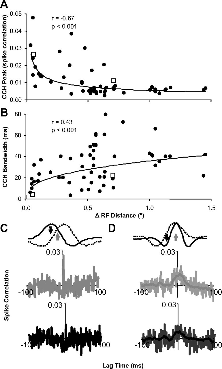
Distance and stimulus dependence of spike correlation properties. A, Scatter plot of the CCH peak height versus distance between receptive field centers for each pair of neurons (n = 63 pairs; power fit). B, Scatter plot of the CCH peak width (half-height) versus distance between receptive field centers for each pair of neurons (n = 63 pairs; power fit). C, D, Example CCHs (A, B, open squares) for overlapping and neighboring receptive fields, respectively, when a disparity was presented that led to a strong response for both neurons (gray) and a stronger response in one neuron relative to the other neuron (black) (n = 60 trials). In D, the light lines in each CCH plot are raw estimates, and the darker lines are smoothed data that were used for any analysis described in the article.

Spike correlation between neurons with receptive distances of <0.5° featured temporally precise spike correlation: strong (Fig. 5A, left), narrow (Fig. 5B, left), and symmetric (Fig. 5C, second row) CCH peaks. These CCHs closely matched the predictions from a model of a common excitatory input (Moore et al., 1970). When these types of neuronal pairs were presented a disparity that was able to drive both neurons equally well (Fig. 5C, top row, gray arrow), a strong narrow CCH peak was observed (Fig. 5C, second row, gray CCH). When a disparity was presented that drove one neuron well, but led to a weak response from the other neuron (Fig. 5C, top row, black arrow), this CCH peak could be reduced in magnitude to a level at which it could not be observed above the CCH noise (Fig. 5C, third row, black CCH).

Spike correlation between neurons with receptive distances of >1.0° featured temporally diffuse spike correlation: weak (Fig. 5A, right) and broad (Fig. 5B, right) CCH peaks (Fig. 5D, second row). These CCHs closely matched predictions from models of a common inhibitory input or more complex polysynaptic excitatory circuits (Moore et al., 1970). The size of these CCH peaks also depended on the disparity presented. The strongest peaks (Fig. 5D, second row, gray CCH) occurred when a disparity was presented that was able to drive both neurons equally well (Fig. 5D, top row, gray arrow). When a disparity was presented that caused a weaker response for one or both neurons (Fig. 5D, top row, black arrow), the CCH peak was usually reduced (Fig. 5D, bottom row, black CCH).

This disparity dependence of spike correlation for the two example pairs of neurons presented in Figure 5 could be explained by firing rate changes that accompany changes in the disparity presented or different circuits being engaged by different disparities presented. We discovered two behaviors of disparity-dependent spike correlation that suggest the latter explanation plays some role because spike correlation varied independently of firing rate.

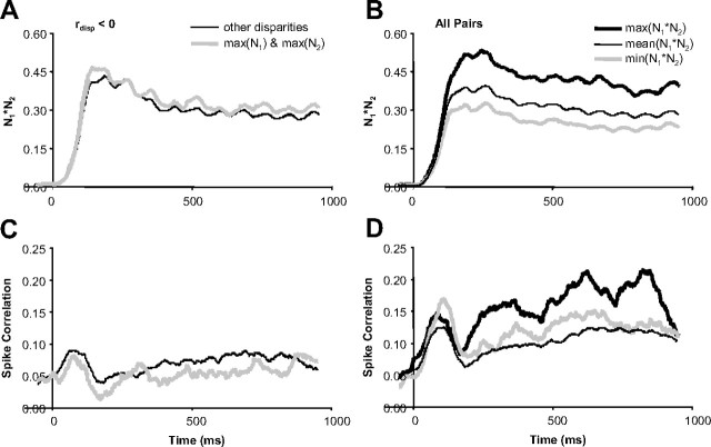
First, for pairs of neurons with very different disparity-tuning (Fig. 5C), we observed the minimum spike correlation at the preferred disparity of one or both of the neurons. These preferred disparities do not typically coincide with low values of N₁*N₂ (the product of the normalized firing rates) and therefore cannot be explained by a dependence of spike correlation on firing rate (de la Rocha et al., 2007). For neurons with r_disp < 0, we computed the average spike correlation at the preferred disparities for each neuron (Fig. 6A; maximum of N₁ and N₂) and compared that to the average spike correlation computed at all other disparities (Fig. 6, left column). We found that the spike correlation was significantly lower at the preferred disparities (n = 17 pairs; p < 0.01) (Fig. 6E) (all statistical tests were paired t tests unless otherwise noted), but N₁*N₂ was not significantly different between the preferred and nonpreferred disparities (p = 0.13) (Fig. 6C). One possible interpretation of this result is that a direct inhibitory connection generating the strongest negative spike correlation at the preferred disparities canceled out the baseline positive spike correlation generated by the common excitatory input.

Figure 6.

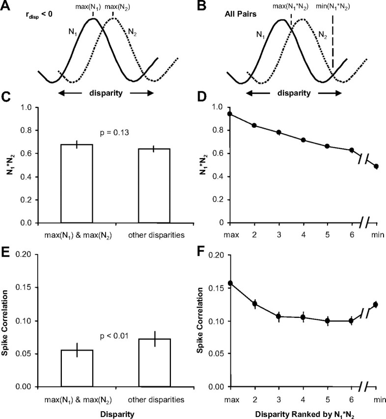
Spike correlation depended on the disparity presented. A, Spike correlation and N₁*N₂ were compared between preferred and nonpreferred disparities. B, Spike correlation and N₁*N₂ were computed for all disparities and ranked by N₁*N₂. Only 7 disparities are shown, because only 7 of the 11 disparities were presented for some pairs of neurons. C, Population average (n = 17 pairs) of N₁*N₂ for the maximum of N₁ and N₂ and all other disparities. D, Population average (n = 63 pairs) of N₁*N₂ sorted by the disparity presented that caused the maximum (max) to the minimum (min) response. E, Population average of spike correlation measurements for the corresponding data presented in C. F, Population average of spike correlation measurements for the corresponding data presented in D. Error bars are population SE.

Second, we observed that spike correlation remained constant or even increased when disparities were presented that led to continually weaker responses in both neurons (lower N₁*N₂), presumably because of common suppression. To summarize this behavior for the population of neuronal pairs, we measured spike correlation for each disparity that was presented. Spike correlation of pairs of neurons depended significantly on the disparity in presented stimuli for 55 of 63 pairs (one-way ANOVA, p < 0.05). For each pair of neurons, the responses were sorted by the disparity presented that caused the greatest product of the normalized firing rates (Fig. 6, right column). Figure 6B displays the population average of N₁*N₂ sorted from the maximum to the minimum. Figure 6D displays the corresponding spike correlation measurements. The falloff of the spike correlation slows as N₁*N₂ continues to decrease at a near-constant rate. The spike correlation then increases for the minimum N₁*N₂. This observation contradicts a simple direct relationship between firing rate and spike correlation because spike correlation could increase for both increasing and decreasing firing rate depending on which disparity was presented. Alternatively, common excitatory circuits could have been engaged when common preferred disparities were presented and common inhibitory circuits when common least preferred disparities were presented. Both circuits would generate positive spike correlation.

Spike correlation varies over time

Spike correlation can also vary over the period of stimulation (Samonds and Bonds, 2005; Zhou et al., 2008). This is also likely attributable to the diversity of the potential circuits contributing to spike correlation between neuronal pairs. Each of the potential circuits described in the previous section can have different temporal dynamics (Angelucci and Bullier, 2003).

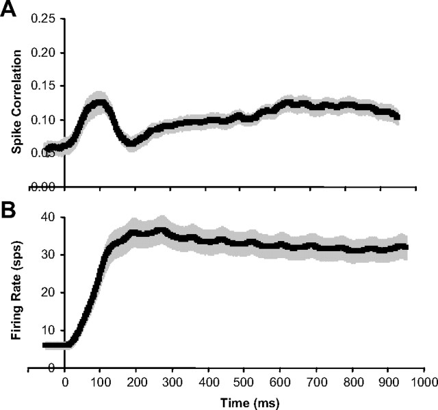
In Figure 7A, we plotted the population average of spike correlation over time (averaged in 100 ms windows). For reference, the population average of the firing rate versus time is plotted in Figure 7B (also averaged in 100 ms windows). At response onset, spike correlation increases at a high rate, is followed by a sharp drop, and then spike correlation slowly increases over the remainder of the stimulation period. The dynamics of the spike correlation are noticeably very distinct from the dynamics of the firing rate.

Figure 7.

Spike correlation varies over time during stimulation. A, Population average of spike correlation versus time (sliding 100 ms windows). B, Population average of firing rate versus time (sliding 100 ms windows). All error bars are population SE (n = 63 neurons). Data for each neuron averaged over all disparities are presented.

We have demonstrated that spike correlation depends on the disparity presented (Figs. 5, 6) and varies over time during stimulation (Fig. 7). The relationship between spike correlation and the disparity presented also varied over time. We show how the same data that was presented in Figure 6 evolved over time in Figure 8. The decrease in spike correlation (Fig. 8C, compare thick gray to thin black line) at the maximum of N₁ and N₂ (Fig. 8A, thick gray line) occurred immediately at the response onset. The increase in spike correlation (Fig. 8D, compare thick gray to thin black line) at the minimum N₁*N₂ (Fig. 8B, thick gray line) was also immediate and strongest during the initial onset burst. The increase in spike correlation (Fig. 8D, compare thick black to thin black line) at the maximum N₁*N₂ (Fig. 8B, thick black line) was strongest in the delayed response after the initial onset burst of both spike correlation and firing rate. The slopes of the spike correlation versus time for the maximum N₁*N₂ were significantly greater than the slopes of the mean spike correlation versus time for all other N₁*N₂ (n = 63 pairs; p < 0.02), as well as the spike correlation versus time at the minimum N₁*N₂ (n = 63 pairs; p < 0.05). These results suggest that the spike correlation changes indicative of suppressive circuits (thick gray) were immediate and therefore local, whereas the spike correlation indicative of facilitative circuits (thick black) were more delayed and therefore distant.

Figure 8.

Timing of spike correlation depended on the disparity presented. A, Population average (n = 17 pairs) of N₁*N₂ versus time for the maximum of N₁ and N₂ and all other disparities. B, Population average (n = 63 pairs) of maximum, mean, and minimum N₁*N₂ versus time. C, Population average of spike correlation versus time for the corresponding data presented in A. D, Population average of spike correlation versus time for the corresponding data presented in B.

Spike correlation depends on disparity-tuning similarity

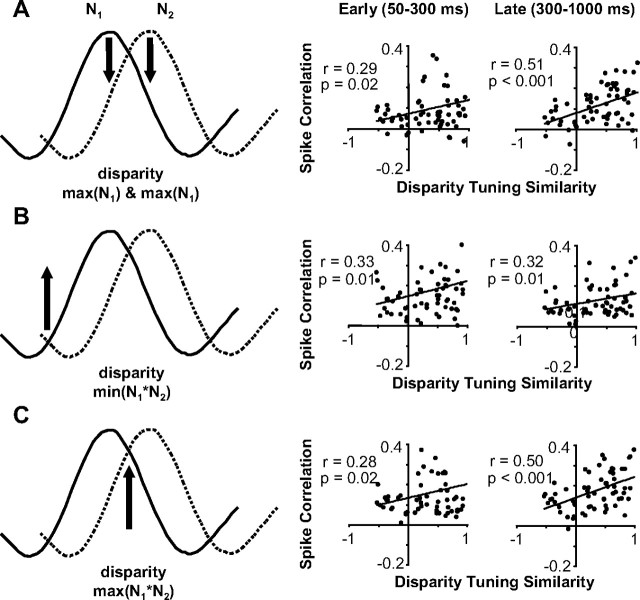
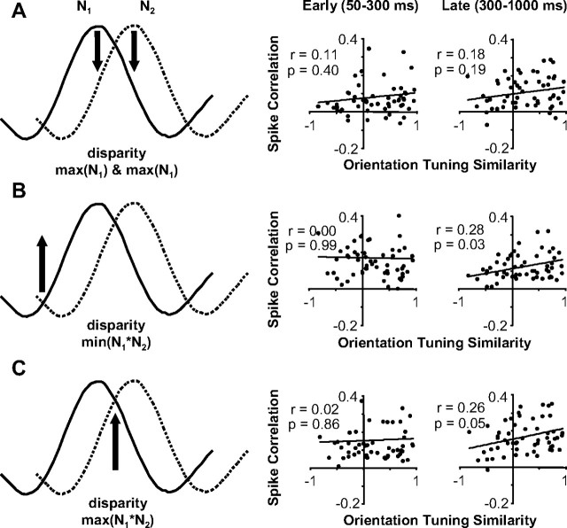
Once we characterized how spike correlation depended on the disparity presented and varied over the period of stimulation, we examined the relationship between the magnitude of spike correlation and disparity-tuning similarity. We summarize the interdependence between disparity-tuning similarity, disparity presented, and time from response onset in Figure 9. Each of three pairs of scatter plots (right column) were generated from data at a particular disparity presented that was computed from the tuning curves (left column). For each pair, scatter plots on the left column are based on the early portion of the response (50–300 ms), whereas plots on the right column include the late portion of the response (300–1000 ms).

Figure 9.

The relationship between spike correlation and disparity-tuning similarity considering disparity presented and response latency. A, Data for all neuronal pairs when a preferred disparity was presented (maximum of N₁ and N₂). Scatter plots of spike correlation versus disparity-tuning similarity for early (50–300 ms; left) and late (300–1000 ms; right) period of stimulation. B, Same organization as A, but for data when the common least preferred disparity was presented (minimum of N₁*N₂). C, Same organization as A, but for data when the common most preferred disparity was presented (maximum of N₁*N₂). All regression analysis was based on n = 63 pairs.

The first pair of scatter plots (Fig. 9A, right) shows the data when a preferred disparity for one neuron was presented: the maximum of N₁ and N₂ or the strongest response from one neuron and a weaker response from the other neuron (Fig. 9A, left). We observed the minimum spike correlation for neuronal pairs with very different disparity tuning and negative spike correlation most often when this disparity was presented, which both are consistent with one neuron suppressing the other neuron. Overall, the net spike correlation was positive, but still weaker than when other disparities were presented (Fig. 9, compare B, C). The spike correlation likely remains positive from a prevalence of common excitatory and inhibitory inputs between V1 neurons strongly influencing spike correlation measurements in general. For this disparity, the spike correlation for neuronal pairs with very similar disparity tuning remained strong because the maximum of N₁ and N₂ was very close to the maximum of N₁*N₂ (Fig. 9, compare A, C). Because pairs of neurons with low r_disp had their minimum spike correlation at this disparity and pairs of neurons with high r_disp had or nearly had their maximum spike correlation at this disparity, we observed a significant dependence between spike correlation and disparity-tuning similarity (n = 63 pairs; r = 0.29 and r = 0.51; p = 0.02 and p < 0.001).

The second pair of scatter plots shows the data when the common least preferred disparity was presented: minimum of N₁*N₂ or a weak response from both neurons (Fig. 9B). Throughout the response, spike correlation was relatively strong and depended on disparity-tuning similarity (n = 63 pairs; r = 0.33 and 0.32; p = 0.01). Pairs of neurons with similar disparity tuning that receive strong common suppression from a neuron tuned to their common least preferred disparity would result in observing stronger positive spike correlation for these pairs relative to other neuronal pairs. The unobserved neuron providing the common suppression would be effectively competing with each neuron by suppressing the responses of the two neurons when driven by its preferred disparity.

The final set of scatter plots shows the data when the mutually preferred disparity was presented: maximum of N₁*N₂ or a strong response from both neurons (Fig. 9C). There was a strong dependence of spike correlation on disparity-tuning similarity especially in the later portion of the response (n = 63 pairs; r = 0.50; p = 0.001).

Disparity tuning of firing rate sharpens over time

In the previous sections, we characterized spike correlation between neuronal pairs tuned for horizontal disparity and compared the behavior of the neurons against the computational predictions of cooperative stereo matching algorithms. In this section, we examine whether or not the firing rate behavior was also consistent with our predictions. To reiterate, we predicted that (1) responses to nonpreferred disparities would be relatively suppressed over time because of competitive interactions and (2) responses to preferred disparities would be relatively enhanced over time because of cooperative interactions. Both behaviors lead to an overall prediction of improved or sharpened disparity tuning over time.

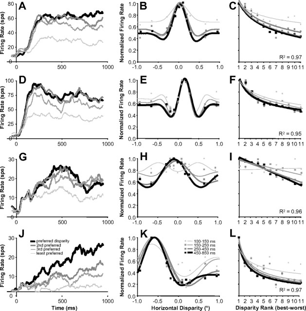
In Figure 10, we present examples of disparity-tuning curves of several neurons and show how the tuning evolves over time. The left column shows the average firing rate over time when different disparities were presented. The responses for several disparities diverge over the stimulation period. Some neurons have very broad tuning (Fig. 10A) early in the response, whereas some neurons had no apparent disparity tuning during the initial response (Fig. 10G). The center column shows the disparity tuning at different time intervals. These intervals were chosen on a log scale because there were more dramatic changes to disparity tuning early in the response. When investigating these examples, we noticed two clear features. First, the responses to the least preferred disparities were increasingly suppressed over time, resulting in enhanced valleys (Fig. 10H) and suppressed secondary peaks (Fig. 10E). Second, the region around the preferred disparity became narrower (Fig. 10B,K). In general, the disparity-tuning curves sharpened over time.

Figure 10.

Disparity tuning improved over time (examples). A, D, G, J, Examples of firing rates over time for preferred and progressively less preferred disparities. B, E, H, K, Disparity-tuning curves of same example neurons computed at progressively later intervals from stimulus onset (Gabor fits). C, F, I, L, Tuning curves of same example neurons ranked from the disparity presented that caused the strongest (best) to the weakest (worst) response (linear, log, and power fits). Note that the vertical axis is the same between the center and right column (peak-normalized firing rate). All average firing rates are based on n = 60 trials.

To summarize this behavior for our population of neurons, we quantified the tuning for disparity continuously and in the same four time intervals we used in Figure 10. Although the Gabor fits used in the center column of Figure 10 illustrate the evolution of disparity tuning very effectively, they do not work well for summarizing the behavior for our population for two main reasons. First, the six-parameter Gabor model does not provide a straightforward single value that represents the two features of disparity-tuning sharpening that we mentioned above. Second, for neurons with weaker responses or poorer disparity tuning, a Gabor model fit was not very stable across time. So to simplify our analysis, we ranked disparities for each neuron based on total spike counts starting with the disparity that elicited the best response to the one that elicited the worst response. Then, we calculated the best linear fit for the data and used the slope as a metric of selectivity for disparity. Because some neurons had a faster falloff in response strength with respect to disparity, we also calculated the slope in log scale for disparity (logarithmic fit) or log scales for both disparity and firing rate (power fit). The fit was chosen based on which fit resulted in the maximum R² (i.e., whichever fit best explained the variance). For 54 of 60 neurons, R² was >0.75 and the median R² was 0.90 (see fits for our examples in the right column in Fig. 10). These fits were not chosen to characterize tuning differences among neurons or disparity tuning in general, but to simply and robustly characterize changes in disparity selectivity of individual neurons over time.

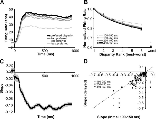
The population average of the example data in the left column and right column of Figure 10 is plotted in Figure 11, A and B, respectively. Figure 11C shows the population average of our slope estimates over time and illustrates how disparity selectivity increases over time. A scatter plot of slopes based on the same time intervals (initial interval vs delayed intervals) used in the center column of Figure 10 reveals that disparity selectivity consistently increases over time (Fig. 11D) (all three sets of points fall below the diagonal; n = 60 neurons; p ≤ 0.002). Different clusters arise along the diagonal axis in Figure 11D because of the different fits (linear, log, power) and demonstrate that the improvements in disparity selectivity occur for neurons with a wide range of disparity tuning (broad-to-narrow). Because the firing rates were normalized by the peak firing rate in each time epoch, the increasing slope means that the ratio of the response for the preferred disparity versus nonpreferred disparities was increasing over time. Therefore, sharpened tuning was not a simple consequence of multiplicative changes in response strength.

Figure 11.

Disparity tuning improved over time (population statistics). A, Population average of firing rate over time for preferred and progressively less preferred disparities. B, Population average of disparity tuning computed at progressively later intervals from stimulus onset (normalized by the peak response in each interval). C, Population average of the slopes computed by linear, log, and power fits of ranked disparity responses over time (rank determined over entire stimulation period). D, Scatter plot of slopes computed at progressively later intervals versus slopes computed during the initial interval. Error bars are population SE (n = 60 neurons).

The results in Figure 11 provide a population summary that captures features such as enhanced valleys (Fig. 10H) and suppressed secondary peaks (Fig. 10E) over time that we observed in the responses of individual neurons. We also examined these two features directly from the population perspective. For 52 of the 60 neurons, there was a secondary peak response away from the preferred disparity (Fig. 12A, dark gray asterisk). In Figure 12B, we plotted the population average of the maximum firing rate (preferred disparity or peak; black), the minimum firing rate (valley; light gray), and the firing rate of secondary peaks (dark gray) versus time. In Figure 12, C and D, the population average of the ratios comparing the peak against the valley (black) and the secondary peak (gray) are plotted versus time. For Figure 12C, we used the difference divided by the sum, which is invariant to multiplicative changes in response strength. For Figure 12D, we used the difference divided by the SD of the tuning curve, which is invariant to multiplicative and additive changes in response strength. We did a logarithmic regression fit on both ratios versus time (from 100 to 1000 ms) for each neuron. As we mentioned when describing Figure 10, we analyzed all sharpening results with respect to time on a log scale because there were more dramatic changes to disparity tuning early in the response. There was a significant positive slope for all four measurements (n = 52 neurons; p < 0.001) supporting that the peak-to-valley was enhanced and the secondary peak was suppressed relative to the primary peak over time, which both cannot be explained by additive changes in the mean firing rate, multiplicative changes in the mean firing rate, or any combination thereof.

Figure 12.

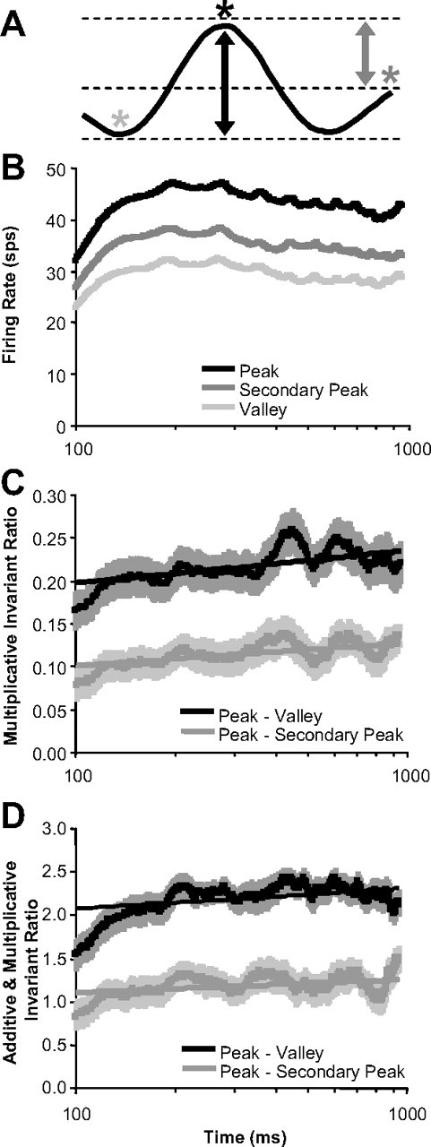
Temporal dynamics of disparity-tuning curve peaks and valleys. A, Schematic of the tuning curve features examined over time. B, Population average of firing rates at the points on the tuning curve described in A (time axis is plotted in log scale). C, Population average of the ratio of firing rates: (peak − valley)/(peak + valley). D, Population average of the ratio of firing rates: (peak − valley)/(SD of the tuning curve). Error bars are population SE (n = 52 neurons), and straight lines are logarithmic regression fit.

Last, we also wanted to assess whether or not the geometry or shape of the tuning curve changed over time (Fig. 10B,K, narrowed peaks). Although the Gabor model does capture the narrowing peak of the disparity-tuning curve with the frequency parameter, we found that it failed to capture other features of disparity-tuning sharpening that we observed. For example, when looking at the disparity-tuning curves computed from data over the entire response duration (Fig. 13A–D), we found that Gabor models were consistently unable to account for peaks being narrower than the valleys in the data (black) because the Gabor function is composed of a single sinusoid (gray). In Figure 13E, we replotted the data from Figure 10K to more clearly show that the peak narrows and the valley broadens over time (compare black to gray data points). Fortunately, sharpening can also be measured directly from the data without fitting each tuning curve to a model. If a tuning curve is sharp, we expect it to have a small number of disparities that yield a very high firing rate, and a large number of disparities that result in a low firing rate. This concept is the same as the statistical measurement of skew. Skewness is the third standardized moment of a distribution and is defined by the following:

where μ₃ is the third moment about the mean, f(d) is the tuning curve (estimated from N disparities), and f̄ and σ denote the mean and SD of the firing rate across that tuning curve. As skewness increases, the number of disparities with proportionately high firing rates decreases, corresponding to an increase in the sharpness of the tuning curve. Skewness is invariant with respect to the mean and variance of the tuning curve. Therefore, changes in skewness cannot be attributed to changes in the baseline firing rate or the amplitude of the tuning curve over time.

Figure 13.

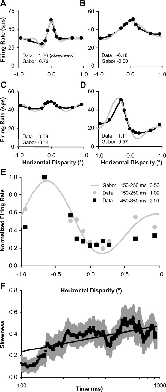
Disparity-tuning skewness increased over time. A–D, Examples of disparity-tuning curves (black) that deviate from fitted Gabor functions (gray). Skewness values for data and Gabor fits are listed in the bottom left corner of each plot. E, Example taken from Figure 10K to demonstrate increasing skewness with respect to time (skewness listed on the right side of the legend). F, Population average of skewness versus time for n = 24 neurons with the most robust disparity tuning (see text). Error bars are population SE, and straight line is logarithmic regression fit.

Skewness was estimated for all the example tuning curves shown in Figure 13 to illustrate that skewness was larger (sharper tuning) for the data versus the Gabor fits and to provide an example of skewness increasing over time. Because skewness achieves its invariance to affine changes of the tuning curve by dividing by the cube of the difference (Eq. 5), we were only able to effectively use it for robust disparity-tuning curves. Noisier tuning curves can lead to spurious very large positive and negative skewness estimates. We measured skewness versus time for the 24 neurons that had disparity discrimination indices (Prince et al., 2002) >0.4. For these 24 neurons, we did a logarithmic regression fit on skewness versus time (for 100–1000 ms) for each neuron and there was a significant positive slope supporting that skewness increased over time (p < 0.01) (Fig. 13F).

Although all of the above measurements were normalized for mean firing rate, the mean firing rates for the different cells did evolve over time (see examples in Fig. 10). An increase in mean firing rate over time coupled with an expansive output nonlinearity that is part of the disparity energy model (e.g., squaring the response) (Ohzawa et al., 1990) could potentially produce sharpened disparity tuning over time. However, these individual examples of mean firing rate over time (Fig. 10) reveal that there was diversity in the temporal profiles. Even though we observed consistent and significant increasing ratios (Fig. 12) and skewness (Fig. 13), we observed no consistent population trend for mean firing rate in this same time interval (n = 52 neurons, p = 0.07, and n = 24 neurons, p = 0.38, respectively). The mean slope versus time for the population of mean firing rates (n = 52 neurons) was negative and significantly less than the mean slopes versus time for all four ratios (p < 0.05). When we examined the time intervals more closely, we found significant examples in which the skewness and mean firing rate were not correlated over time. For example, in Figure 10, there were significant increases in skewness (p < 0.05; bootstrapped with respect to trials) between time intervals not only when the mean firing rate increased (Fig. 10J) (p < 0.001), but also when it decreased (Fig. 10D; p < 0.05) or did not significantly change (Fig. 10A) (p = 0.78). Even in the case in which skewness increased while mean firing rate increased (Figs. 10J, 13E), the change in shape of the tuning curve over this period could not be explained by an expansive output nonlinearity such as squaring the output. Although it is possible that the sharpened disparity tuning of some neurons resulted from an increase in mean firing rate coupled with an expansive output nonlinearity, the sharpened tuning of other neurons was likely caused by other nonlinear behavior such as network interactions.

Spike correlation depends on orientation-tuning similarity

Several anatomical studies have revealed that horizontal or lateral synaptic connections among V1 neurons are constrained to pairs with similar orientation tuning (Gilbert and Weisel, 1989; Malach et al., 1993; Bosking et al., 1997; Lund et al., 2003). Therefore, similar to the relationship between spike correlation and disparity-tuning similarity that we observed, spike correlation increases for pairs of neurons with more similar orientation tuning (Samonds et al., 2006; Smith and Kohn, 2008). Examining the relationship between spike correlation and orientation-tuning similarity can provide additional support that the measurement of spike correlation reflects the underlying neuronal circuitry. In addition, by comparing the spike correlation relationships based on disparity-tuning similarity to orientation-tuning similarity, we could determine to what extent our spike correlation measurements could be explained by the previous anatomical and neurophysiological studies. The similarity of the dynamics of disparity tuning constrained spike correlation and the sharpening of disparity tuning based on firing rate suggests that the behaviors are linked. This link would imply that the spike correlation–disparity-tuning relationships that we have described could not be explained by orientation-tuning similarity constrained connectivity. However, examining the two relationships directly would more clearly distinguish our spike correlation results from those based on orientation tuning.

We examined the relationship between spike correlation and orientation-tuning similarity (Fig. 14) for our data in the same manner as when using disparity-tuning similarity as the metric (compare Fig. 9). For disparities that result in spike correlation that we are interpreting as suppressive (preferred disparity for one neuron; nonpreferred for the other neuron), there is no significant dependence on orientation-tuning similarity (Fig. 14A). For disparities that result in increased spike correlation for neuronal pairs with minimum or maximum N₁*N₂, the spike correlation also did not depend on orientation-tuning similarity early in the response (Fig. 14B,C, center column). However, later in the response, we did find that spike correlation was stronger for neuronal pairs with more similar orientation tuning (Fig. 14B,C, right column). Differences between results for the early and late portion of the response occurred even if a portion of the late response equal to the early response was analyzed. Last, the probability of finding significant spike correlation was significantly greater for neuronal pairs with similar orientation preferences (p < 0.05; Wilcoxon's rank sum test for tuning properties of n = 63 interacting vs n = 91 non-interacting pairs). Overall, the results are consistent with previous research by showing that stronger spike correlation occurs between pairs of neurons with more similar orientation tuning.

Figure 14.

The relationship between spike correlation and orientation-tuning similarity considering disparity presented and response latency (during DRDS presentation). A, Data for all neuronal pairs when a preferred disparity was presented (maximum of N₁ and N₂). Scatter plots of spike correlation versus orientation-tuning similarity for early (50–300 ms; left) and late (300–1000 ms; right) period of stimulation. B, Same organization as A, but for data when the common least preferred disparity was presented (minimum of N₁*N₂). C, Same organization as A, but for data when the common most preferred disparity was presented (maximum of N₁*N₂). All regression analysis was based on n = 63 pairs.

Our result of increased spike correlation for more similar disparity tuning (Fig. 9), however, cannot be explained by the orientation-tuning-based results (Fig. 14) because there was no significant relationship between disparity- and orientation-tuning similarity (r = 0.03; p = 0.80). So, although our spike correlation measurements do capture previously documented organization with respect to orientation tuning in V1, the data also reveal a new dimension of organization based on disparity tuning that might be involved in sharpening disparity tuning over time.

Discussion

We observed several trends in the characteristics of spike correlation and the temporal dynamics of the responses for disparity-tuned neurons in V1 that are consistent with a cooperative computational strategy for stereo matching (Sperling, 1970; Dev, 1975; Nelson, 1975; Marr and Poggio, 1976; Pollard et al., 1985; Prazdny, 1985). The observations can be grouped with respect to evidence of suppressive or facilitative interactions among disparity-tuned neurons.

Evidence of suppressive interactions

First, spike correlation was negative or decreased relative to baseline immediately after response onset when neuronal pairs of distinct disparity tuning were presented a “competitive disparity” (i.e., disparity that results in the maximum response in one neuron and a weaker response in the other neuron) (Figs. 3C, 8C). This reduced spike correlation was observed as disparity tuning became more distinct. We also observed a trend of increased spike correlation for neurons with more similar disparity tuning when common least preferred disparities were presented to neuronal pairs (Fig. 9B). This increased positive spike correlation could be caused by stronger common suppression. Both neurons that we were observing could be receiving a suppressive input from a neuron that we did not record from that is tuned to a competing disparity. Last, we observed that firing rates to nonpreferred disparities were reduced relative to the responses to other disparities over the course of the response (Figs. 10–13), which is also consistent with suppression from neurons with competing preferred disparities. These three pieces of evidence are consistent with suppressive interactions, and because we observed the evidence soon after response onset (Figs. 3C, 8C), they are consistent with local interactions.

Evidence of facilitative interactions

First, spike correlation was positive and increased after response onset when neuronal pairs were presented stimuli with mutually preferred disparities, suggesting that there was facilitation among these pairs (Figs. 3F, 8D). This facilitation was specific or stronger for neuronal pairs with similar disparity tuning (Fig. 9C) and was present even over longer distances in which receptive fields do not overlap (Fig. 4). Second, we observed sharpening of disparity tuning, suggesting that the response of the preferred disparity was enhanced relative to the responses to nonpreferred disparities over time (Figs. 10–13). These two results could be a consequence of positive reinforcement among neurons tuned for similar disparities. Because the spike correlation increased at long delays and was observed for neuronal pairs with nonoverlapping receptive fields, this suggests that the reinforcement was being propagated over distances large enough to include neurons that have neighboring and distinct receptive fields.

Relationship to previous V1 studies

We observed that spike correlation depended on the disparity presented and varied over the stimulation period. Numerous studies in V1 have revealed dynamic behavior using similar (Singer, 1999; Kohn and Smith, 2005) or identical (Samonds and Bonds, 2005; Zhou et al., 2008) spike correlation measures as in the present study. Some of this behavior could be attributed to firing-rate dependence of spike correlation as a result of the spiking threshold (de la Rocha et al., 2007) and refractory period (Ito and Tsuji, 2000), but other observed changes in spike correlation occur even when firing rates remain constant (Singer, 1999). Our results also reveal changes in spike correlation that were independent of firing rate changes. First, spike correlation increased for both firing rate increases and decreases (Figs. 6, 8). Second, the temporal dynamics of spike correlation and firing rate were distinct (Figs. 7, 8).

Computational studies have proposed hypotheses about how this feature-dependent spike correlation might have consequences in encoding information among V1 networks (Singer, 1999; Samonds et al., 2004, 2006; Montani et al., 2007; Shea-Brown et al., 2008). The present analysis was to attempt to clarify the potential underlying circuits that generate spike correlation and how they might influence disparity tuning. When making spike correlation measurements, we cannot interpret the results without considering the stimulus-dependent aspects of these measurements.

Positive spike correlation has been observed for a variety of neuronal pairs in V1, but most noticeable for neurons with similar orientation tuning (Ts'o et al., 1986; Singer, 1999; Samonds et al., 2006; Smith and Kohn, 2008). Direct inhibitory connections and suppressive interactions within V1 tend to be local (Lund et al., 2003) and sometimes specific and sometimes nonspecific with respect to orientation tuning (Bosking et al., 1997; Das and Gilbert, 1999; Shapley et al., 2003). Excitatory interactions intrinsic to V1 can extend over greater distances and are restricted to occur among neurons with similar orientation tuning (Ts'o et al., 1986; Gilbert and Weisel, 1989; Malach et al., 1993; Bosking et al., 1997; Singer, 1999; Lund et al., 2003). Extrastriate feedback also extends over greater distances but is not specific with respect to orientation tuning (Stettler et al., 2002). If we assume that early spike correlation reflects local inhibitory circuits and late spike correlation reflects distant intrinsic excitatory circuits, we reach similar conclusions as these studies about the behavior of spike correlation when considering disparity-tuning relationships and reveal a new dimension to V1 circuitry.

We also found similarities to previous V1 studies that examined the temporal dynamics of neuronal activity. Experimental and analytical differences limit a direct comparison to the study by Shapley et al. (2003), which found that orientation tuning sharpened over time, but our observation that disparity tuning sharpened over time might be related to similar mechanisms. With respect to our spike correlation measurements, Smith and Kohn (2008) and Zhou et al. (2008) found similar transient and slowly increasing spike count correlation, spike correlation, and spike coherence. In the study by Shapley et al. (2003), the underlying circuitry was inferred based on models that could generate the dynamics of orientation tuning that they observed experimentally. In the studies by Smith and Kohn (2008) and Zhou et al. (2008), spike count correlation, spike correlation, and spike coherence were not examined in the context of orientation-tuning sharpening. In the present study, we provide a more complete view of the relationship between the dynamics of tuning and spike correlation. The similarity of these two independent circuits that might be involved in improving orientation and disparity tuning may be part of a more general inference process in V1. Computational and psychophysical studies suggest that computations of horizontal disparity could be facilitated by computations of orientation (van Ee and Anderson, 2001; Ben-Shahar et al., 2003).

Limitations of interpretations

We provided evidence of neuronal interactions based on spike correlation measurements and evidence of sharpening of disparity tuning over time. We proposed that the two events are linked, but sharpened disparity tuning coinciding with an increase in mean firing rate could potentially be explained by the expansive output nonlinearity in the disparity energy model (Ohzawa et al., 1990) and does not necessarily imply neuronal interactions. However, we observed sharpening of disparity-tuning curves in neurons when their mean firing rates decreased or did not change. This observation suggests that the expansive output nonlinearity cannot fully explain all the sharpening effects.

Nonetheless, the evidence of the proposed link between spike correlation and tuning sharpening is suggestive rather than direct evidence. This is because disparity tuning is a consequence of several thousand inputs to a single neuron and each spike correlation measurement is between only two neurons that are connected directly or most likely indirectly. The dynamics of spike correlation measurements will depend highly on the spacing between the two recording electrodes, whereas the dynamics of disparity tuning will not. However, we produced a neuronal network model constrained by the spike correlation data to examine the dynamics of the disparity tuning in the model and compare it to the data from recorded neurons (Samonds et al., 2007, 2008). Interestingly, this model could account for the deviation of observed disparity-tuning curves from predictions of the local disparity energy model (Fig. 13) (Cumming and Parker, 1997; Prince et al., 2002; Cumming and Thomas, 2007; Samonds et al., 2007). By examining spike correlation characteristics, single-neuron disparity-tuning dynamics, and neuronal network model behavior simultaneously, we strengthen our argument versus if we examined each aspect independently.

Our suggestion that the observed interactions among neurons are attributable to cooperative stereo computations is not necessarily incompatible with proposed models based on direct feedforward mechanisms (Ohzawa et al., 1990; Fleet et al., 1996; Qian and Zhu, 1997; Tsai and Victor, 2003; Chen and Qian, 2004). The neuronal interactions can combine with and complement local feedforward disparity-tuning computations (Ohzawa et al., 1990; DeAngelis et al., 1991; Cumming and DeAngelis, 2001; Prince et al., 2002; Parker, 2007) to reduce their uncertainty. Cooperative computations can coexist with local feedforward interactions (Menz and Freeman, 2003) as suggested in some models (Marr and Poggio, 1979). Finally, our data are not conclusive with respect to cooperative stereo computations and are also consistent with alternative computational approaches that predict neuronal interactions among disparity-tuned neurons (Lehky and Sejnowski, 1990; Stevenson et al., 1992; Read and Cumming, 2007). Additional experiments will be necessary to elucidate the computational significance of the general neuronal interactions that we observed.

Conclusions

Stereopsis is an example of the general problem of visual inference under uncertainty. When viewing an image through a small aperture (equivalent to a V1 receptive field), we cannot determine whether the local image is part of an object, its direction of movement, or its depth. The solution to this problem necessarily involves integrating information from multiple receptive fields across space. Simply pooling information over space by averaging sacrifices the resolution of individual neurons. Global constraints combined with local competition can more efficiently and effectively integrate visual information over space. This strategy is ubiquitous to visual inference and early visual computations in general (Marr, 1982). In this article, we provided evidence suggesting that such integration could play an important computational role in solving the stereo correspondence problem.

References

- Aertsen AM, Gerstein GL, Habib MK, Palm G. Dynamics of neuronal firing correlation: modulation of “effective connectivity.”. J Neurophysiol. 1989;61:900–917. doi: 10.1152/jn.1989.61.5.900. [DOI] [PubMed] [Google Scholar]
- Angelucci A, Bullier J. Reaching beyond the classical receptive field of V1 neurons: horizontal or feedback axons? J Physiol Paris. 2003;97:141–154. doi: 10.1016/j.jphysparis.2003.09.001. [DOI] [PubMed] [Google Scholar]
- Bair W, Zohary E, Newsome WT. Correlated firing in macaque visual area MT: time scales and relationship to behavior. J Neurosci. 2001;21:1676–1697. doi: 10.1523/JNEUROSCI.21-05-01676.2001. [DOI] [PMC free article] [PubMed] [Google Scholar]
- Ben-Shahar O, Huggins PS, Izo T, Zucker SW. Cortical connections and early visual function: intra- and inter-columnar processing. J Physiol Paris. 2003;97:191–208. doi: 10.1016/j.jphysparis.2003.09.004. [DOI] [PubMed] [Google Scholar]
- Bosking WH, Zhang Y, Schofield B, Fitzpatrick D. Orientation selectivity and the arrangement of horizontal connections in tree shrew striate cortex. J Neurosci. 1997;17:2112–2127. doi: 10.1523/JNEUROSCI.17-06-02112.1997. [DOI] [PMC free article] [PubMed] [Google Scholar]
- Brody CD. Disambiguating different covariation types. Neural Comput. 1999;11:1527–1535. doi: 10.1162/089976699300016124. [DOI] [PubMed] [Google Scholar]
- Chen Y, Qian N. A coarse-to-fine disparity energy model with both phase-shift and position-shift receptive field mechanisms. Neural Comput. 2004;16:1545–1577. doi: 10.1162/089976604774201596. [DOI] [PubMed] [Google Scholar]
- Collett TS. Extrapolating and interpolating surfaces in depth. Proc R Soc Lond B Biol Sci. 1985;224:43–56. doi: 10.1098/rspb.1985.0020. [DOI] [PubMed] [Google Scholar]
- Cumming BG, DeAngelis GC. The physiology of stereopsis. Annu Rev Neurosci. 2001;24:203–238. doi: 10.1146/annurev.neuro.24.1.203. [DOI] [PubMed] [Google Scholar]
- Cumming BG, Parker AJ. Responses of primary visual cortical neurons to binocular disparity without depth perception. Nature. 1997;389:280–283. doi: 10.1038/38487. [DOI] [PubMed] [Google Scholar]
- Cumming BG, Thomas OM. Dynamics of responses to anticorrelated disparities in primate V1 suggest recurrent network interactions. Soc Neurosci Abstr. 2007;33:716–1. [Google Scholar]
- Das A, Gilbert CD. Topography of contextual modulations mediated by short-range interactions in primary visual cortex. Nature. 1999;399:655–661. doi: 10.1038/21371. [DOI] [PubMed] [Google Scholar]
- DeAngelis GC, Ohzawa I, Freeman RD. Depth is encoded in the visual cortex by a specialized receptive field structure. Nature. 1991;352:156–159. doi: 10.1038/352156a0. [DOI] [PubMed] [Google Scholar]
- de la Rocha J, Doiron B, Shea-Brown E, Josić K, Reyes A. Correlation between neural spike trains increases with firing rate. Nature. 2007;448:802–806. doi: 10.1038/nature06028. [DOI] [PubMed] [Google Scholar]
- Dev P. Perception of depth surfaces in random-dot stereograms: a neural model. Int J Man Mach Stud. 1975;7:511–528. [Google Scholar]
- Eckhorn R, Bauer R, Jordan W, Brosch M, Kruse W, Munk M, Reitboeck HJ. Coherent oscillations: a mechanism for feature linking in visual cortex? Biol Cybern. 1988;60:121–130. doi: 10.1007/BF00202899. [DOI] [PubMed] [Google Scholar]
- Efron B, Tibshirani R. An introduction to the bootstrap. London: Chapman and Hall; 1993. [Google Scholar]
- Fleet DJ, Wagner H, Heeger DJ. Neural encoding of binocular disparity: energy models, position shifts and phase shifts. Vision Res. 1996;36:1839–1857. doi: 10.1016/0042-6989(95)00313-4. [DOI] [PubMed] [Google Scholar]
- Gerstein GL, Kirkland KL. Neural assemblies: technical issues, analysis, and modeling. Neural Netw. 2001;14:589–598. doi: 10.1016/s0893-6080(01)00042-9. [DOI] [PubMed] [Google Scholar]
- Gilbert CD, Wiesel TN. Columnar specificity of intrinsic horizontal and corticocortical connections in cat visual cortex. J Neurosci. 1989;9:2432–2442. doi: 10.1523/JNEUROSCI.09-07-02432.1989. [DOI] [PMC free article] [PubMed] [Google Scholar]
- Gray CM, König P, Engel AK, Singer W. Oscillatory responses in cat visual cortex exhibit inter-columnar synchronization which reflects global stimulus properties. Nature. 1989;338:334–337. doi: 10.1038/338334a0. [DOI] [PubMed] [Google Scholar]
- Ito H, Tsuji S. Model dependence in quantification of spike interdependence by joint peri-stimulus time histogram. Neural Comp. 2000;12:195–217. doi: 10.1162/089976600300015952. [DOI] [PubMed] [Google Scholar]
- Julesz B, Chang J-J. Interaction between pools of binocular disparity detectors tuned to different disparities. Biol Cybern. 1976;22:107–119. doi: 10.1007/BF00320135. [DOI] [PubMed] [Google Scholar]
- Kapadia MK, Ito M, Gilbert CD, Westheimer G. Improvement in visual sensitivity by changes in local context: parallel studies in human observers and in V1 of alert monkeys. Neuron. 1995;15:843–856. doi: 10.1016/0896-6273(95)90175-2. [DOI] [PubMed] [Google Scholar]
- Kelly RC, Smith MA, Samonds JM, Kohn A, Bonds AB, Movshon JA, Lee TS. Comparison of recordings from microelectrode arrays and single electrodes in the visual cortex. J Neurosci. 2007;27:261–264. doi: 10.1523/JNEUROSCI.4906-06.2007. [DOI] [PMC free article] [PubMed] [Google Scholar]
- Kohn A, Smith MA. Stimulus dependence of neuronal correlation in primary visual cortex of the macaque. J Neurosci. 2005;25:3661–3673. doi: 10.1523/JNEUROSCI.5106-04.2005. [DOI] [PMC free article] [PubMed] [Google Scholar]
- Lehky SR, Sejnowski TJ. Neural model of stereoacuity and depth interpolation based on a distributed representation of stereo disparity. J Neurosci. 1990;10:2281–2299. doi: 10.1523/JNEUROSCI.10-07-02281.1990. [DOI] [PMC free article] [PubMed] [Google Scholar]
- Lund JS, Angelucci A, Bressloff PC. Anatomical substrates for functional columns in macaque monkey primary visual cortex. Cereb Cortex. 2003;13:15–24. doi: 10.1093/cercor/13.1.15. [DOI] [PubMed] [Google Scholar]
- Malach R, Amir Y, Harel M, Grinvald A. Relationship between intrinsic connections and functional architecture revealed by optical imaging and in vivo targeted biocytin injections in primate striate cortex. Proc Natl Acad Sci U S A. 1993;90:10469–10473. doi: 10.1073/pnas.90.22.10469. [DOI] [PMC free article] [PubMed] [Google Scholar]
- Marr D. Vision. San Francisco: Freeman; 1982. [Google Scholar]
- Marr D, Poggio T. Cooperative computation of stereo disparity. Science. 1976;194:283–287. doi: 10.1126/science.968482. [DOI] [PubMed] [Google Scholar]
- Marr D, Poggio T. A computational theory of human stereo vision. Proc R Soc Lond B Biol Sci. 1979;204:301–328. doi: 10.1098/rspb.1979.0029. [DOI] [PubMed] [Google Scholar]
- Menz MD, Freeman RD. Stereoscopic depth processing in the visual cortex: a coarse-to-fine mechanism. Nat Neurosci. 2003;6:59–65. doi: 10.1038/nn986. [DOI] [PubMed] [Google Scholar]
- Mitchison GJ, McKee SP. Interpolation in stereoscopic matching. Nature. 1985;315:402–404. doi: 10.1038/315402a0. [DOI] [PubMed] [Google Scholar]
- Montani F, Kohn A, Smith MA, Schultz SR. The role of correlations in direction and contrast coding in primary visual cortex. J Neurosci. 2007;27:2338–2348. doi: 10.1523/JNEUROSCI.3417-06.2007. [DOI] [PMC free article] [PubMed] [Google Scholar]
- Moore GP, Segundo JP, Perkel DH, Levitan H. Statistical signs of synaptic interactions in neurons. Biophys J. 1970;10:876–900. doi: 10.1016/S0006-3495(70)86341-X. [DOI] [PMC free article] [PubMed] [Google Scholar]
- Nelson JI. Globality and stereoscopic fusion in binocular vision. J Theor Biol. 1975;49:1–88. doi: 10.1016/s0022-5193(75)80020-8. [DOI] [PubMed] [Google Scholar]
- Ohzawa I, DeAngelis GC, Freeman RD. Stereoscopic depth discrimination in the visual cortex: neurons ideally suited as disparity detectors. Science. 1990;249:1037–1041. doi: 10.1126/science.2396096. [DOI] [PubMed] [Google Scholar]
- Parker AJ. Binocular depth perception and the cerebral cortex. Nat Rev Neurosci. 2007;8:379–391. doi: 10.1038/nrn2131. [DOI] [PubMed] [Google Scholar]
- Pollard SB, Mayhew JE, Frisby JP. PMF: a stereo correspondence algorithm using a disparity gradient limit. Perception. 1985;14:449–470. doi: 10.1068/p140449. [DOI] [PubMed] [Google Scholar]
- Prazdny K. Detection of binocular disparities. Biol Cybern. 1985;52:93–99. doi: 10.1007/BF00363999. [DOI] [PubMed] [Google Scholar]
- Prince SJ, Cumming BG, Parker AJ. Range and mechanism of encoding of horizontal disparity in macaque V1. J Neurophysiol. 2002;87:209–221. doi: 10.1152/jn.00466.2000. [DOI] [PubMed] [Google Scholar]
- Qian N, Zhu Y. Physiological computation of binocular disparity. Vision Res. 1997;37:1811–1827. doi: 10.1016/s0042-6989(96)00331-8. [DOI] [PubMed] [Google Scholar]
- Ramachandran VS, Cavanaugh P. Subjective contours capture stereopsis. Nature. 1985;317:527–530. [Google Scholar]
- Read JC, Cumming BG. Sensors for impossible stimuli may solve the stereo correspondence problem. Nat Neurosci. 2007;10:1322–1328. doi: 10.1038/nn1951. [DOI] [PMC free article] [PubMed] [Google Scholar]
- Ringach DL, Hawken MJ, Shapley R. Dynamics of orientation tuning in macaque primary visual cortex. Nature. 1997;387:281–284. doi: 10.1038/387281a0. [DOI] [PubMed] [Google Scholar]
- Samonds JM, Bonds AB. Gamma oscillation maintains stimulus structure-dependent synchronization in cat visual cortex. J Neurophysiol. 2005;93:223–236. doi: 10.1152/jn.00548.2004. [DOI] [PubMed] [Google Scholar]
- Samonds JM, Allison JD, Brown HA, Bonds AB. Cooperative synchronized assemblies enhance orientation discrimination. Proc Natl Acad Sci U S A. 2004;101:6722–6727. doi: 10.1073/pnas.0401661101. [DOI] [PMC free article] [PubMed] [Google Scholar]
- Samonds JM, Zhou Z, Bernard MR, Bonds AB. Synchronous activity in cat visual cortex encodes collinear and cocircular contours. J Neurophysiol. 2006;95:2602–2616. doi: 10.1152/jn.01070.2005. [DOI] [PubMed] [Google Scholar]
- Samonds JM, Potetz BR, Lee TS. Implications of neuronal interactions on disparity tuning in V1. Soc Neurosci Abstr. 2007;33:716.4. [Google Scholar]
- Samonds JM, Potetz BR, Poplin RE, Lee TS. Neuronal interactions reduce local feature uncertainty. Soc Neurosci Abstr. 2008;34:568.14. [Google Scholar]
- Shapley R, Hawken M, Ringach DL. Dynamics of orientation selectivity in the primary visual cortex and the importance of cortical inhibition. Neuron. 2003;38:689–699. doi: 10.1016/s0896-6273(03)00332-5. [DOI] [PubMed] [Google Scholar]
- Shea-Brown E, Josić K, de la Rocha J, Doiron B. Correlation and synchrony transfer in integrate-and-fire neurons: basic properties and consequences for coding. Phys Rev Lett. 2008;100:108102. doi: 10.1103/PhysRevLett.100.108102. [DOI] [PubMed] [Google Scholar]
- Shoham S, Fellows MR, Normann RA. Robust, automatic spike sorting using a mixtures of multivariate t-distributions. J Neurosci Methods. 2003;127:111–122. doi: 10.1016/s0165-0270(03)00120-1. [DOI] [PubMed] [Google Scholar]
- Singer W. Neuronal synchrony: a versatile code review for the definition of relations? Neuron. 1999;24:49–65. 111–125. doi: 10.1016/s0896-6273(00)80821-1. [DOI] [PubMed] [Google Scholar]
- Smith MA, Kohn A. Spatial and temporal scales of neuronal correlation in primary visual cortex. J Neurosci. 2008;28:12591–12603. doi: 10.1523/JNEUROSCI.2929-08.2008. [DOI] [PMC free article] [PubMed] [Google Scholar]
- Smith MA, Kelly RC, Lee TS. Dynamics of response to perceptual pop-out stimuli in macaque V1. J Neurophysiol. 2007;98:3436–3449. doi: 10.1152/jn.00441.2007. [DOI] [PubMed] [Google Scholar]
- Sperling G. Binocular vision: a physiological and neural theory. Am J Psychol. 1970;83:461–534. [Google Scholar]
- Stettler DD, Das A, Bennett J, Gilbert CD. Lateral connectivity and contextual interactions in macaque primary visual cortex. Neuron. 2002;36:739–750. doi: 10.1016/s0896-6273(02)01029-2. [DOI] [PubMed] [Google Scholar]
- Stevenson SB, Cormack LK, Schor CM. Depth attraction and repulsion in random dot stereograms. Vision Res. 1991;31:805–813. doi: 10.1016/0042-6989(91)90148-x. [DOI] [PubMed] [Google Scholar]
- Stevenson SB, Cormack LK, Schor CM, Tyler CW. Disparity tuning in mechanisms of human stereopsis. Vision Res. 1992;32:1685–1694. doi: 10.1016/0042-6989(92)90161-b. [DOI] [PubMed] [Google Scholar]
- Tsai JJ, Victor JD. Reading a population code: a multi-scale neural model for representing binocular disparity. Vision Res. 2003;43:445–466. doi: 10.1016/s0042-6989(02)00510-2. [DOI] [PubMed] [Google Scholar]
- Ts'o DY, Gilbert CD, Wiesel TN. Relationships between horizontal interactions and functional architecture in cat striate cortex as revealed by cross-correlation analysis. J Neurosci. 1986;6:1160–1170. doi: 10.1523/JNEUROSCI.06-04-01160.1986. [DOI] [PMC free article] [PubMed] [Google Scholar]
- van Ee R, Anderson BL. Motion direction, speed and orientation in binocular matching. Nature. 2001;410:690–694. doi: 10.1038/35070569. [DOI] [PubMed] [Google Scholar]
- Ventura V, Cai C, Kass RE. Trial-to-trial variability and its effect on time-varying dependency between two neurons. J Neurophysiol. 2005a;94:2928–2939. doi: 10.1152/jn.00644.2004. [DOI] [PubMed] [Google Scholar]
- Ventura V, Cai C, Kass RE. Statistical assessment of time-varying dependency between two neurons. J Neurophysiol. 2005b;94:2940–2947. doi: 10.1152/jn.00645.2004. [DOI] [PubMed] [Google Scholar]
- Westheimer G. Spatial interaction in the domain of disparity signals in human stereoscopic vision. J Physiol. 1986;370:619–629. doi: 10.1113/jphysiol.1986.sp015954. [DOI] [PMC free article] [PubMed] [Google Scholar]
- Zhou Z, Bernard MR, Bonds AB. Deconstruction of spatial integrity in visual stimulus detected by modulation of synchronized activity in cat visual cortex. J Neurosci. 2008;28:3759–3768. doi: 10.1523/JNEUROSCI.4481-07.2008. [DOI] [PMC free article] [PubMed] [Google Scholar]