Frequency Diffeomorphisms for Efficient Image Registration

Abstract

This paper presents an efficient algorithm for large deformation diffeomorphic metric mapping (LDDMM) with geodesic shooting for image registration. We introduce a novel finite dimensional Fourier representation of diffeomorphic deformations based on the key fact that the high frequency components of a diffeomorphism remain stationary throughout the integration process when computing the deformation associated with smooth velocity fields. We show that manipulating high dimensional diffeomorphisms can be carried out entirely in the bandlimited space by integrating the nonstationary low frequency components of the displacement field. This insight substantially reduces the computational cost of the registration problem. Experimental results show that our method is significantly faster than the state-of-the-art diffeomorphic image registration methods while producing equally accurate alignment. We demonstrate our algorithm in two different applications of image registration: neuroimaging and in-utero imaging.

1 Introduction

Diffeomorphisms have been widely used in the field of image registration [6, 7], atlas-based image segmentation [4,10], and anatomical shape analysis [14, 22]. In this paper, we focus on a time-varying velocity field representation for diffeomorphisms as it supplies a distance metric that is critical to statistical analysis of anatomical shapes, for instance, by least squares, geodesic regression, or principal modes detection [13,16,22].

In spite of the advantages of supporting Riemannian metrics in LDDMM, the extremely high computational cost and large memory footprint of the current implementations has limited the use of time-varying velocity representations in important applications that require computational efficiency. The original LDDMM optimization performs gradient decent on the entire time-varying velocity field that is defined on a dense image grid. Since a geodesic is uniquely determined by its initial conditions on the velocity field, the geodesic shooting algorithm has been shown to reduce the computational complexity and improve optimization landscape by manipulating the initial velocity via the geodesic evolution equations [20]. FLASH (finite dimensional Lie algebras for shooting) [23] is a recent variant of LDDMM with geodesic shooting that employs a low dimensional bandlimited representation of the initial velocity field to further improve the convergence and efficiency of the optimization. The algorithm still maps the velocity fields from the low dimensional Fourier space back to the full image domain to perform forward integration at each iteration [23]. The computational complexity of this step thus dominates the entire procedure of diffeomorphic image registration.

Previous works that aimed to improve diffeomorphic representations have reduced the high degrees of freedom available to represent the velocity fields, but not the diffeomorphisms themselves. In this paper, we adopt the low dimensional representation of the tangent space of diffeomorphisms [23] and propose an efficient way to compute diffeomorphisms in the bandlimited space, thus further reducing the computational complexity of image registration. Our approach is based on the important insight that only the low frequency components of the diffeomorphisms vary over time when integrating a bandlimited velocity field to obtain the deformation. Since the optimization of image registration can be directly solved by advecting the inverse of diffeomorphisms [17], we propose a novel Fourier representation of the deformation in the inverse coordinate system that is computed entirely in the low dimensional bandlimited space. The theoretical tools developed in this paper are broadly applicable to other parametrization of diffeomorphic transformations, such as stationary velocity fields [2,3,19]. To evaluate the proposed algorithm, we perform image registration of real 3D MR images and show that the accuracy of the propagated segmentations is comparable to that obtained via the state-of-the-art diffeomorphic image registration methods, while the runtime and the memory demands are dramatically lower for our method. We demonstrate the method in the context of atlas-based segmentation of brain images and of temporal alignment of in-utero MRI scans.

2 Background

Before introducing our development, we provide a brief overview of continuous diffeomorphisms endowed with metrics on vector fields [6,21] and of the finite dimensional Fourier representation of the tangent space of diffeomorphisms [23].

Given an open and bounded d-dimensional domain Ω ⊂ ℝ^d, we use Diff(Ω) to denote a space of continuous differentiable and inverse differentiable mappings of Ω onto itself. The distance metric between the identity element e and any diffeomorphism ϕ

$$\text{dist}(e,\varphi )={\displaystyle {\int }_0^1(\mathcal{L}{v}_t,v_t)dt}$$ (1)

depends on the time-varying Eulerian velocity field v_t (t ∈ [0, 1]) in the tangent space of diffeomorphisms V = T Diff(Ω). Here ℒ : V → V* is a symmetric, positive-definite differential operator, e.g., discrete Laplacian, with its inverse $\mathcal{K}:V\ast \to V$, and m_t ∈ V* is a momentum vector that lies in the dual space V* such that m_t = ℒv_t and $v_t=\mathcal{K}{m}_t$.

The path of deformation fields ϕ_t parametrized by t ∈ [0, 1] is generated by

$$\frac{d{\varphi }_t}{dt}=v_t\circ {\varphi }_t,$$ (2)

where ○ is a composition operator. The inverse mapping of ϕ_t is defined via

$$\frac{d{\varphi }_t^{-1}}{dt}=-D{\varphi }_t^{-1}\cdot v_t,$$ (3)

where D is the d × d Jacobian matrix at each voxel and · is an element-wise multiplication.

The geodesic shooting algorithm estimates the initial velocity at t = 0 and relies on the fact that a geodesic path of transformations ϕ_t and its inverse ${\varphi }_t^{-1}$ with a given initial condition v₀ can be uniquely determined through integrating the Euler-Poincaré differential equation (EPDiff) [1,12] as

$$\frac{\partial v_t}{\partial t}=-\mathcal{K}[{(D{v}_t)}^T{m}_t+D{m}_t{v}_t+m_t\text{div}(v_t)],$$ (4)

where div is the divergence operator and $\mathcal{K}$ is a smoothing operator that guarantees the smoothness of the velocity fields.

2.1 Fourier Representation of Velocity Fields

Let f : ℝ^d → ℝ be a real-valued function. The Fourier transform ℱ of f is given by

$$\mathcal{F}[f]({\xi }_1,\dots ,{\xi }_d)={\displaystyle {\int }_{{\mathrm{ℝ}}^d}f(x_1,\dots ,x_d)e^{-2\pi i(x_1{\xi }_1+\dots +x_d{\xi }_d)}d{x}_1,\dots ,d{x}_d,}$$ (5)

where (ξ₁, …, ξ_d) is a d-dimensional frequency vector. The inverse Fourier transform ℱ⁻¹ of a discretized Fourier signal $\stackrel{\sim }{f}$

$${\mathcal{F}}^{-1}[\stackrel{\sim }{f}](x_1,\dots ,x_d)={\displaystyle \sum _{{\xi }_1,\dots ,{\xi }_d}\stackrel{\sim }{f}({\xi }_1,\dots ,{\xi }_d)e^{2\pi i({\xi }_1{x}_1+\dots +{\xi }_d{x}_d)}}$$ (6)

is an approximation of the original signal f. To ensure that $\stackrel{\sim }{f}$ represents a real-valued vector field in the spatial domain, we require $\stackrel{\sim }{f}({\xi }_1,\dots ,{\xi }_d)=\stackrel{\sim }{f}\ast (-{\xi }_1,\dots ,-{\xi }_d)$, where * denotes the complex conjugate. When working with vector-valued functions of diffeomorphisms ϕ and velocity fields v, we apply the Fourier transform to each vector component separately.

Since $\mathcal{K}$ is a smoothing operator that suppresses high frequencies in the Fourier domain, the geodesic evolution Eq. (4) suggests that the velocity field v_t can be represented efficiently as a bandlimited signal in Fourier space. Let $\stackrel{\sim }{V}$ denote the discrete Fourier space of velocity fields. As shown in [23], for any two elements $\stackrel{\sim }{v}$, $\stackrel{\sim }{w}\in \stackrel{\sim }{V}$, the distance metric at identity $\stackrel{\sim }{e}$ is defined as

$${\langle \stackrel{\sim }{u},\stackrel{\sim }{v}\rangle }_{\stackrel{\sim }{V}}={\displaystyle \int (\stackrel{\sim }{\mathcal{L}}\stackrel{\sim }{v}(\xi ),\stackrel{\sim }{w}(\xi ))d\xi ,}$$

where $\stackrel{\sim }{\mathcal{L}}:\stackrel{\sim }{V}\mapsto \stackrel{\sim }{V}\ast$ is the Fourier transform of a commonly used Laplacian operator (−αΔ + e)^c, with a positive weight parameter α and a smoothness parameter c, i.e.,

$$\stackrel{\sim }{\mathcal{L}}({\xi }_1,\dots ,{\xi }_d)={\left[-2\alpha {\displaystyle \sum _{j=1}^d(\cos (2\pi {\xi }_j)-1)+1}\right]}^c.$$

The Fourier representation of the inverse operator $\mathcal{K}:\stackrel{\sim }{V}\ast \mapsto \stackrel{\sim }{V}$ is equal to $\stackrel{\sim }{\mathcal{K}}({\xi }_1,\dots ,{\xi }_d)={\stackrel{\sim }{\mathcal{L}}}^{-1}({\xi }_1,\dots ,{\xi }_d)$.

Therefore, the geodesic shooting Eq. (4) can be efficiently computed in a low dimensional bandlimited velocity space:

$$\frac{\partial {\stackrel{\sim }{v}}_t}{\partial t}=-\stackrel{\sim }{\mathcal{K}}\left[{(\stackrel{\sim }{D}{\stackrel{\sim }{v}}_t)}^T★{\stackrel{\sim }{m}}_t+\stackrel{\sim }{\nabla }\cdot ({\stackrel{\sim }{m}}_t\otimes {\stackrel{\sim }{v}}_t)\right],$$ (7)

where ★ is the truncated matrix-vector field auto-correlation and $\stackrel{\sim }{D}{\stackrel{\sim }{v}}_t$ is a tensor product $\stackrel{\sim }{D}\otimes {\stackrel{\sim }{v}}_t$ with $\stackrel{\sim }{D}({\xi }_1,\dots ,{\xi }_d)=(i\sin (2\pi {\xi }_1),\dots ,i\sin (2\pi {\xi }_d))$ representing the Fourier frequencies of a central difference Jacobian matrix D. Operator $\stackrel{\sim }{\nabla }\cdot$ is the discrete divergence of a vector field $\stackrel{\sim }{v}$, which is computed as the sum of the Fourier coefficients of the central difference operator $\stackrel{\sim }{D}$ along each dimension, i.e., $\stackrel{\sim }{\nabla }\cdot ({\xi }_1,\dots ,{\xi }_d)={\displaystyle \sum _{j=1}^{d}i\sin (2\pi {\xi }_j)}$.

3 Frequency Diffeomorphisms and Signal Decomposition

While geodesic shooting in the Fourier space (7) is efficient, integrating the ordinary differential Eq. (2) to compute the corresponding diffeomorphism from a velocity field remains computationally intensive. To address this problem, we introduce a Fourier representation of diffeomorphisms that is simple and easy to manipulate in the bandlimited space. The proposed representation promises improved computational efficiency of any algorithm that requires generation of diffeomorphisms from velocity fields.

Analogous to the continuous inverse flow in (3), we define a sequence of time-dependent inverse diffeomorphisms ${\varphi }_t^{-1}$ in the Fourier domain that consequently generates a path of geodesic flow. Because that the pointwise multiplication of two vector fields in the spatial domain corresponds to convolution in the Fourier domain, we can easily compute the multiplication of a square matrix and a vector field in the Fourier domain as a single convolution for each row of the matrix.

Let $\stackrel{\sim }{\text{Diff}}(\Omega )$ denote the space of Fourier representations of diffeomorphisms. To simplify the notation, we use ψ ≜ ϕ⁻¹ in the remainder of this section. Given time-dependent velocity field ${\stackrel{\sim }{v}}_t\in \stackrel{\sim }{V}$, the diffeomorphism ${\stackrel{\sim }{\psi }}_t\in \stackrel{\sim }{\text{Diff}}(\Omega )$ in the finite-dimensional Fourier domain can be computed as

$$\frac{d{\stackrel{\sim }{\psi }}_t}{dt}=-\stackrel{\sim }{D}{\stackrel{\sim }{\psi }}_t\ast {\stackrel{\sim }{v}}_t,$$ (8)

where * is a circular convolution with zero padding to avoid aliasing. To prevent the domain from growing infinity, we truncate the output of the convolution in each dimension to a suitable finite set.

Representing diffeomorphisms entirely in the Fourier space eliminates the effort of converting their associated velocity fields back and forth from the Fourier domain to the spatial domain. While current implementations of computing a diffeomorphism in (3) have complexity O(N^d) on a full image grid of linear size N, the complexity of naively integrating (8) is O(N^d log N) if the convolution operator is implemented via fast Fourier transform (FFT) [18]. Here we show how to reduce the complexity of (8) via frequency decomposition of the deformations.

In particular, we consider a representation $\stackrel{\sim }{\psi }=\stackrel{\sim }{e}+\stackrel{\sim }{u}$, where $\stackrel{\sim }{e}$ is the Fourier transform of the identity transformation, and ũ is the Fourier transform of the displacement field. We can now isolate the frequency response of the identity transformation in (8) as follows:

$$\frac{d{\stackrel{\sim }{\psi }}_t}{dt}=-\stackrel{\sim }{D}(\stackrel{\sim }{e}+{\stackrel{\sim }{u}}_t)\ast {\stackrel{\sim }{v}}_t=\stackrel{\sim }{D}\stackrel{\sim }{e}\ast {\stackrel{\sim }{v}}_t-\stackrel{\sim }{D}{\stackrel{\sim }{u}}_t\ast {\stackrel{\sim }{v}}_t.$$ (9)

Since De · v_t = v_t in the spatial domain, we have

$$\stackrel{\sim }{D}\stackrel{\sim }{e}\ast {\stackrel{\sim }{v}}_t=\mathcal{F}(De\cdot v_t)=\mathcal{F}(v_t)={\stackrel{\sim }{v}}_t.$$ (10)

Substituting (10) into (9), we arrive at

$$\frac{d{\stackrel{\sim }{\psi }}_t}{dt}=-{\stackrel{\sim }{v}}_t-\stackrel{\sim }{D}{\stackrel{\sim }{u}}_t\ast {\stackrel{\sim }{v}}_t\text{with}{\stackrel{\sim }{\psi }}_0=\stackrel{\sim }{e},\text{or}$$

$${\stackrel{\sim }{u}}_t=-{\displaystyle {\int }_0^t{\stackrel{\sim }{v}}_{\tau }}+\stackrel{\sim }{D}{\stackrel{\sim }{u}}_{\tau }\ast {\stackrel{\sim }{v}}_{\tau }d\tau \text{with}{\stackrel{\sim }{u}}_0=0.$$ (11)

Importantly, we observe that the high frequency components of the diffeomorphisms that come from the initial condition ${\stackrel{\sim }{\psi }}_0=\stackrel{\sim }{e}$ remain unchanged, and only low frequency components vary throughout the integration. Moreover, the evolution scheme for geodesic shooting in the Fourier domain (7) indeed maintains ${\stackrel{\sim }{v}}_t$ as a bandlimited signal. The truncated convolution operation does not introduce high frequencies if the displacement ũ_t is also bandlimited. Figure 1 illustrates a 1D example of the integration (11).

Fig. 1.

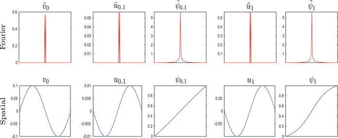
A 1D example of an initial velocity v₀ as a sinusoid function and the resulting displacement field u_t and diffeomorphism ψ_t at t = 0.1 and t = 1. Both Fourier (red) and spatial (blue) representations are shown. (Color figure online)

The initial condition ${\stackrel{\sim }{\psi }}_0=\stackrel{\sim }{e}$ corresponds to ũ₀ = 0. We first integrate (11) for bandlimited low frequency components of the signal and then add the high frequency components back. Therefore we have

$$\text{for}\xi \le \eta ,{\stackrel{\sim }{u}}_t(\xi )=-{\displaystyle {\int }_0^t{\stackrel{\sim }{v}}_{\tau }(\xi )}+\stackrel{\sim }{D}{\stackrel{\sim }{u}}_{\tau }(\xi )\ast {\stackrel{\sim }{v}}_{\tau }(\xi )d\tau ,$$

$$\text{for}\xi >\eta ,{\stackrel{\sim }{u}}_t(\xi )=0,$$ (12)

where ξ = (ξ₁, …, ξ_d) and η = (η₁, …, η_d) is the vector of upper bounds on the frequency in the bandlimited representation of ψ.

3.1 Frequency Diffeomorphisms for Image Registration

In this section, we present a diffeomorphic image registration algorithm based on geodesic shooting that is carried out entirely in the Fourier space.

Let S be the source image and T be the target image defined on a torus domain Γ = ℝ^d/ℤ^d (S(x), T(x) : Γ → ℝ). The problem of diffeomorphic image registration is to find the shortest path of diffeomorphisms ψ_t ∈ Diff(Γ) : Γ → Γ, t ∈ [0, 1] such that S○ψ₁ is similar to T, where ○ is a composition operator that resamples S by the smooth mapping ψ₁. LDDMM with geodesic shooting [20] leads to a gradient decent optimization of an explicit energy function

$$E(v_0)=\frac{\mathrm{\lambda }}{2}\text{dist}(S\circ {\psi }_1,T)+\frac{1}{2}{\Vert v_0\Vert }_V^2$$ (13)

under the constraints (2) and (4). The distance function dist(·,·) measures the dissimilarity between images. Commonly used distance metrics include sum-of-squared difference (L²-norm) of image intensities, normalized cross correlation (NCC), and mutual information (MI). Here λ > 0 is a weight parameter.

The energy function in the finite-dimensional Fourier space can be equivalently formulated as

$$E({\stackrel{\sim }{v}}_0)=\frac{\mathrm{\lambda }}{2}\text{dist}(S\circ {\psi }_1,T)+\frac{1}{2}{\Vert {\stackrel{\sim }{v}}_0\Vert }_{\stackrel{\sim }{V}}^2$$ (14)

with the new constraints (7) and (8).

We use a gradient decent algorithm on the initial velocity ${\stackrel{\sim }{v}}_0$ to estimate the path of diffeomorphic flow $\left\{{\stackrel{\sim }{\psi }}_t\right\}$ entirely in the bandlimited space. Beginning with the initialization ${\stackrel{\sim }{v}}_0=0$, the gradient of the energy (14) is computed via two steps below:

1. Compute the gradient ${\nabla }_{{\stackrel{\sim }{v}}_1}E$ of the energy (14) at t = 1. This requires integrating both the diffeomorphism ${\stackrel{\sim }{\psi }}_t$ and the velocity field ${\stackrel{\sim }{v}}_t$ forward in time, and then mapping ${\stackrel{\sim }{\psi }}_1$ to the spatial domain to obtain ψ₁. Formally,

   $${\nabla }_{{\stackrel{\sim }{v}}_1}E=\mathcal{K}\mathcal{F}\left(\frac{\partial \text{dist}(S\circ {\psi }_1,T)}{\partial (S\circ {\psi }_1)}\cdot \nabla (S\circ {\psi }_1)\right).$$ (15)
2. Bring the gradient ${\nabla }_{{\stackrel{\sim }{v}}_1}E$ in (15) back to t = 0 by reduced adjoint Jacobi field equations [8,23]. Integrate the reduced adjoint Jacobi field equations

   $$\frac{d\widehat{v}}{dt}=-{\text{ad}}_{\stackrel{\sim }{v}}^{†}\widehat{h},\frac{d\widehat{h}}{dt}=-\widehat{v}-{\text{ad}}_{\stackrel{\sim }{v}}\widehat{h}+{\text{ad}}_{\widehat{h}}^{†}\stackrel{\sim }{v}$$ (16)

   in $\stackrel{\sim }{V}$ to get the gradient update ${\nabla }_{{\stackrel{\sim }{v}}_0}E$, where ad^† is an adjoint operator and $\widehat{v}$, $\widehat{h}\in \stackrel{\sim }{V}$ are introduced adjoint variables.

The algorithm is summarized below.

Algorithm 1.

Frequency diffeomorphisms for image registration

Input: source image S, target image T.

Initialize ${\widehat{v}}_0=0$.

repeat

(a) Integrate (7) to compute ${\widehat{v}}_t$ at discrete time points t = [0, …, 1].

(b) Integrate (8) to generate ${\stackrel{\sim }{\psi }}_t$.

(ci) Convert ${\stackrel{\sim }{\psi }}_1$ back to the spatial domain to transport the source image S.

(cii) Compute the gradient ${\nabla }_{{\stackrel{\sim }{v}}_1}E$ (15) at time point t = 1.

(d) Integrate ${\nabla }_{{\stackrel{\sim }{v}}_1}E$ backward in time via (16) to obtain ${\nabla }_{{\stackrel{\sim }{v}}_0}E$.

(e) Update ${\widehat{v}}_0\leftarrow {\widehat{v}}_0-\delta {\nabla }_{{\stackrel{\sim }{v}}_0}E$, where δ is the step size.

until convergence

Computational Complexity

It has previously been shown that the complexity of steps (a) and (d) is O(Tn^d), where T is the number of time steps in the integration and n is the truncated dimension in the bandlimited space. The complexity of the current methods for computing diffeomorphisms in the high-dimensional image space via (2) is O(T N^d). In contrast, our algorithm reduces the complexity of this step to O(Tn^d) (step (b)). To transport the images and measure the image dissimilarity at t = 1, we convert the transformation ${\stackrel{\sim }{\psi }}_1$ into the spatial domain via FFT (O(N^d log N)) (step (c_i)). While the theoretical complexity of FFT is higher than the complexity of computing $S\circ {\psi }_1^{-1}$, which is O(N^d), its empirical runtime for N a power of 2 is quite low by comparison. Figure 2 reports the empirical runtime of FFT and of linear interpolation for different image grid sizes (N = 2⁷, 2⁸, 2⁹) as used by the current methods and ours to transport S. We note that the linear interpolation requires more than twice the amount of time than that of FFT.

Fig. 2.

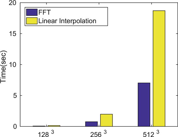
Exact run-time of FFT (blue) and linear interpolation (yellow). (Color figure online)

4 Experimental Evaluation

To evaluate the proposed approach, we perform registration-based segmentation and examine the resulting segmentation accuracy, runtime and memory consumption of the algorithm. We compare the proposed method with the diffeomorphic demons implementation in ANTS software package [5] and the state-of-the-art fast geodesic shooting for LDDMM method FLASH [23] (downloaded from: https://bitbucket.org/FlashC/flashc). In all experiments, we set α = 1.5, c = 3.0, λ = 1.0e4 and T = 10 for the time integration. A normalized cross correlation (NCC) metric for image dissimilarity and a multi-resolution optimization scheme with three levels are used in all three methods. To evaluate volume overlap between the propagated segmentation A and the manual segmentation B for each structure, we compute the Dice Similarity Coefficient DSC(A, B) = 2(|A| ∩ |B|)/(|A| + |B|) where ∩ denotes an intersection of two regions.

4.1 Data

We evaluate the method on 3D brain MRI scans [9] and 4D in-utero MRI time series [11].

3D Brain MRI

Thirty six brain MRI scans (T1-weighted MP-RAGE) were acquired in normal subjects and patients with Alzhimer’s disease across a broad age range. The MRI images are of dimension 256³, 1 mm isotropic voxels and were computed by averaging three or four scans. All scans underwent skull stripping, intensity normalization, bias field correction, and co-registration with affine transformation. An atlas was built from 20 images as a reference. Manual segmentations are available for all scans in the set. We perform image registration of the 3D brain atlas to the remaining 16 subjects. We evaluate registration by examining the accuracy of atlas-based delineations for white matter (WM), cortex (Cor), ventricles (Vent), hippocampus (Hipp), and caudate (Caud).

4D In-Utero Time-Series Volumetric MRI

Ten pregnant women (three singleton pregnancies, six twin pregnancies, and one triplet pregnancy) were recruited and consented. Single-shot GRE-EPI image series were acquired for each woman on a 3T MR scanner (Skyra Siemens, 18-channel body and 12-channel spine receive arrays, 3 × 3 mm² in-plane resolution, 3 mm slice thickness, interleaved slice acquisition, TR = 5.8 − 8 s, TE = 32 − 36 ms, FA = 90°). Odd and even slices of each volume were resampled onto an isotropic 3 mm³ image grid to reduce the effects of interleaved acquisition. Each series includes around 300 3D volumes. The placentae (total of 10) and fetal brains (total of 18) were manually delineated in the reference template and in five additional volumes in each series. When applying our method to in-utero MRI, we use it as part of sequential registration of the consecutive frames in the scan series. Each series requires about 300 consecutive image registration steps over time.

4.2 Results

3D Brain MRI

Figure 3 reports the total energy (14) averaged over 16 test images for different values of truncated dimension n = 8, 16, ⋯, 128. Our method arrives at the same solution at n = 32 and higher. For the remainder of this section, we use n = 32 to illustrate the results. An example segmentation obtained by our algorithm is also illustrated in Fig. 3. Figure 4 reports the volume overlap of segmentations for our method and the two baseline algorithms. All three algorithms produce comparable segmentation accuracy. The difference is not statistically significant in a paired t-test for each labelled structure (p = 0.369). Our algorithm has substantially lower computational cost than ANTS and FLASH. Figure 4 also provides runtime and memory consumption across all methods.

Fig. 3.

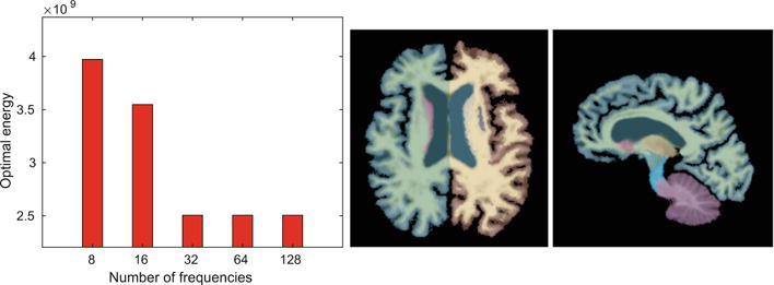
Left: average final energy for different values of the truncated dimension n = 8, 16, …, 128. Right: example propagated segmentation with 35 structures obtained by our method. 2D slices are shown for visualization only, all computations are carried out fully in 3D.

Fig. 4.

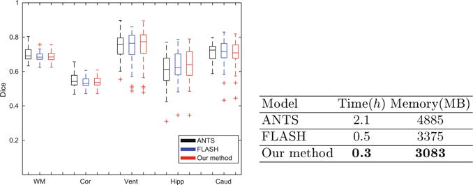
Left: volume overlap between atlas-based and manual segmentations for five important regions (white matter, cortex, ventricles, hippocampus, and caudate) estimated via ANTS (black), FLASH (blue), and our method (red). Right: Runtime and memory consumption per image for all three methods. (Color figure online)

4D In-Utero Time-Series Volumetric MRI

Similar to the previous experiment, we cross-validated the optimal truncated dimension n at different scales and set n = 16 for the 4D in-utero time series. Once all the volumes in the series are aligned, we transform the manual segmentations in the first volume to other volumes in each series by using the estimated deformations. Figure 5 illustrates results for an example case from the study. We observe that the delineations achieved by transferring manual segmentations from the reference frame to the coordinate system of the target frame 25 align fairly well with the manual segmentations. Figure 6 reports segmentation volume overlap for the fetal brains and placenta, as well as the time and memory consumption for our method and the two baseline algorithms. Again, our algorithm achieves comparable results (paired t-test p = 0.4671) while offering significant improvements in computational efficiency.

Fig. 5.

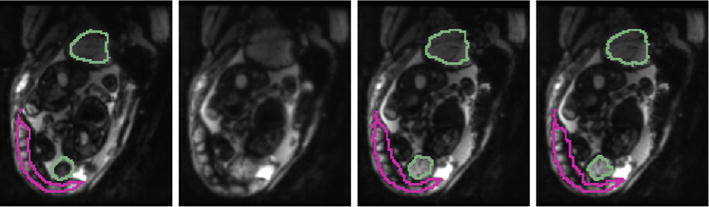
An example case from the in-utero MRI study. Left to right: source with manual segmentation, deformed source, target with manual segmentation, and target with propagated segmentations for the fetal brains (green) and placenta (pink). 2D slices of axial view are shown for visualization only, all computations are carried out fully in 3D. (Color figure online)

Fig. 6.

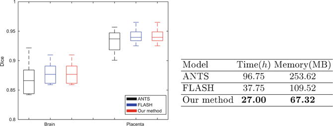
Left: volume overlap between transferred and manual segmentations of fetal brains and placenta averaged over all subjects. Statistics are reported for ANTS (black), FLASH (blue), and our method (red). Right: Runtime and memory consumption of 300 registrations for all three algorithms. (Color figure online)

5 Conclusion

We presented an efficient way to compute diffeomorphisms in the setting of LDDMM with geodesic shooting for image registration. Our method is the first to represent diffeomorphisms in the Fourier space, which provides a way to compute transformations from the associated velocity fields entirely in the low dimensional bandlimited space. This approach reduces the computational cost of the algorithms without loss in accuracy. The theoretical tools employed in this work are not only broadly applicable to other representations of diffeomorphic transformations such as stationary velocity fields, but also to the standard path optimization strategy in the original LDDMM. Our method can be naturally interpreted as operating with the left-invariant metric on the space of diffeomorphisms [15], which accepts spatially-varying smoothing kernels in special image registration scenarios where different regularizations are required at different locations. Future research will explore more of numerical analysis, as well as its theoretical connection and implications for diffeomorphic image registration.

References

- 1.Arnol’d VI. Sur la géométrie différentielle des groupes de Lie de dimension infinie et ses applications à l’hydrodynamique des fluides parfaits. Ann Inst Fourier. 1966;16:319–361. [Google Scholar]
- 2.Arsigny V, Commowick O, Pennec X, Ayache N. A log-Euclidean framework for statistics on diffeomorphisms. In: Larsen R, Nielsen M, Sporring J, editors. MICCAI 2006 LNCS. Vol. 4190. Springer; Heidelberg: 2006. pp. 924–931. [DOI] [PubMed] [Google Scholar]
- 3.Ashburner J. A fast diffeomorphic image registration algorithm. Neuroimage. 2007;38(1):95–113. doi: 10.1016/j.neuroimage.2007.07.007. [DOI] [PubMed] [Google Scholar]
- 4.Ashburner J, Friston KJ. Unified segmentation. Neuroimage. 2005;26(3):839–851. doi: 10.1016/j.neuroimage.2005.02.018. [DOI] [PubMed] [Google Scholar]
- 5.Avants BB, Epstein CL, Grossman M, Gee JC. Symmetric diffeomorphic image registration with cross-correlation: evaluating automated labeling of elderly and neurodegenerative brain. Med Image Anal. 2008;12(1):26–41. doi: 10.1016/j.media.2007.06.004. [DOI] [PMC free article] [PubMed] [Google Scholar]
- 6.Beg M, Miller M, Trouvé A, Younes L. Computing large deformation metric mappings via geodesic flows of diffeomorphisms. Int J Comput Vis. 2005;61(2):139–157. [Google Scholar]
- 7.Christensen GE, Rabbitt RD, Miller MI. Deformable templates using large deformation kinematics. IEEE Tran Image Process. 1996;5(10):1435–1447. doi: 10.1109/83.536892. [DOI] [PubMed] [Google Scholar]
- 8.Francesco B. Invariant affine connections and controllability on lie groups. California Institute of Technology; 1995. (Technical report for Geometric Mechanics). [Google Scholar]
- 9.Johnson KA, Jones K, Holman BL, Becker JA, Spiers PA, Satlin A, Albert MS. Preclinical prediction of Alzheimer’s disease using spect. Neurology. 1998;50(6):1563–1571. doi: 10.1212/wnl.50.6.1563. [DOI] [PubMed] [Google Scholar]
- 10.Joshi S, Davis B, Jomier M, Gerig G. Unbiased diffeomorphic atlas construction for computational anatomy. NeuroImage. 2004;23(Supplement 1):151–160. doi: 10.1016/j.neuroimage.2004.07.068. [DOI] [PubMed] [Google Scholar]
- 11.Liao R, Turk EA, Zhang M, Luo J, Grant PE, Adalsteinsson E, Golland P. Temporal registration in in-utero volumetric MRI time series. In: Ourselin S, Joskowicz L, Sabuncu MR, Unal G, Wells W, editors. MICCAI 2016 LNCS. Vol. 9902. Springer; Cham: 2016. pp. 54–62. [DOI] [PMC free article] [PubMed] [Google Scholar]
- 12.Miller MI, Trouvé A, Younes L. Geodesic shooting for computational anatomy. J Math Imaging Vis. 2006;24(2):209–228. doi: 10.1007/s10851-005-3624-0. [DOI] [PMC free article] [PubMed] [Google Scholar]
- 13.Niethammer M, Huang Y, Vialard FX. Geodesic regression for image time-series. In: Fichtinger G, Martel A, Peters T, editors. MICCAI 2011 LNCS. Vol. 6892. Springer; Heidelberg: 2011. pp. 655–662. [DOI] [PMC free article] [PubMed] [Google Scholar]
- 14.Qiu A, Younes L, Miller MI. Principal component based diffeomorphic surface mapping. Med Imaging IEEE Trans. 2012;31(2):302–311. doi: 10.1109/TMI.2011.2168567. [DOI] [PMC free article] [PubMed] [Google Scholar]
- 15.Schmah T, Risser L, Vialard FX. Diffeomorphic image matching with left-invariant metrics. In: Chang DE, Holm DD, Patrick G, Ratiu T, editors. Geometry, Mechanics, and Dynamics. Springer; New york: 2015. pp. 373–392. [Google Scholar]
- 16.Singh N, Fletcher PT, Preston JS, Ha L, King R, Marron JS, Wiener M, Joshi S. Multivariate statistical analysis of deformation momenta relating anatomical shape to neuropsychological measures. In: Jiang T, Navab N, Pluim JPW, Viergever MA, editors. MICCAI 2010 LNCS. Vol. 6363. Springer; Heidelberg: 2010. pp. 529–537. [DOI] [PubMed] [Google Scholar]
- 17.Singh N, Vialard FX, Niethammer M. Splines for diffeomorphisms. Med Image Anal. 2015;25(1):56–71. doi: 10.1016/j.media.2015.04.012. [DOI] [PubMed] [Google Scholar]
- 18.Van Loan C. Computational Frameworks for the Fast Fourier Transform. Vol. 10. SIAM; Philadelphia: 1992. [Google Scholar]
- 19.Vercauteren T, Pennec X, Perchant A, Ayache N. Diffeomorphic demons: efficient non-parametric image registration. NeuroImage. 2009;45(1):S61–S72. doi: 10.1016/j.neuroimage.2008.10.040. [DOI] [PubMed] [Google Scholar]
- 20.Vialard FX, Risser L, Rueckert D, Cotter CJ. Diffeomorphic 3D image registration via geodesic shooting using an efficient adjoint calculation. Int J Comput Vis. 2012;97:229–241. [Google Scholar]
- 21.Younes L, Arrate F, Miller M. Evolutions equations in computational anatomy. NeuroImage. 2009;45(1S1):40–50. doi: 10.1016/j.neuroimage.2008.10.050. [DOI] [PMC free article] [PubMed] [Google Scholar]
- 22.Zhang M, Fletcher PT. Bayesian principal geodesic analysis in diffeomorphic image registration. In: Golland P, Hata N, Barillot C, Hornegger J, Howe R, editors. MICCAI 2014 LNCS. Vol. 8675. Springer; Cham: 2014. pp. 121–128. [DOI] [PubMed] [Google Scholar]
- 23.Zhang M, Fletcher PT. Finite-dimensional lie algebras for fast diffeomorphic image registration. In: Ourselin S, Alexander DC, Westin C-F, Cardoso MJ, editors. IPMI 2015 LNCS. Vol. 9123. Springer; Cham: 2015. pp. 249–260. [DOI] [PubMed] [Google Scholar]