Mapping causal variants with single nucleotide resolution reveals biochemical drivers of phenotypic change

Summary

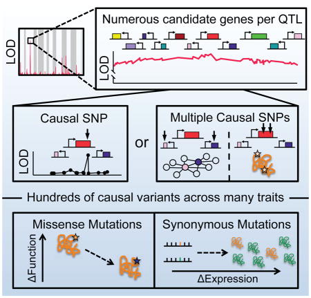
Understanding the sequence determinants that give rise to diversity among individuals and species is the central challenge of genetics. Despite ever-greater numbers of sequenced genomes, most genome-wide association studies cannot distinguish causal variants from linked passenger mutations spanning many genes. We report that this inherent challenge can be overcome in model organisms. By pushing the advantages of inbred crossing to its practical limit in Saccharomyces cerevisiae, we improved the statistical resolution of linkage analysis to single nucleotides. This ‘super-resolution’ approach allowed us to map 370 causal variants across 26 quantitative traits. Missense, synonymous, and cis-regulatory mutations collectively gave rise to phenotypic diversity, providing mechanistic insight into the basis of evolutionary divergence. Our data also systematically unmasked complex genetic architectures, revealing that multiple closely linked driver mutations frequently act on the same quantitative trait. Single-nucleotide mapping thus complements traditional deletion and overexpression screening paradigms and opens new frontiers in quantitative genetics.

Graphical Abstract

A roadmap is presented for obtaining a systematic quantitative understanding between genotype and phenotype at single nucleotide resolution

INTRODUCTION

Genetics is not destiny. However, the DNA polymorphisms that are inherited in families can affect our risk for disease, the physical dimensions of our bodies, and even our baseline behavioral tendencies (Visscher et al., 2012). Long before physical genomes could be fully sequenced, the early pioneers of quantitative genetics scoured the genome for mutations responsible for the most extreme manifestations of these traits (Botstein et al., 1980; Donis-Keller et al., 1987). By harnessing the power of family pedigrees, investigators linked unique restriction endonuclease sites to disease alleles, creating the first linkage maps of our genomes (Hall et al., 1990).

Although linkage was a blessing that allowed geneticists to pinpoint genes responsible Mendelian diseases, it is now a curse for the vast majority of heritable traits, which are influenced by many variants of small effect (Manolio et al., 2009). Identifying these variants is hampered by the sparsity of meiotic crossovers. Even in a highly outbred human population, the average size of a haplotype block spans dozens of polymorphisms (Frazer et al., 2007; Gabriel et al., 2002), meaning that each causal polymorphism is inherited along with numerous statistically indistinguishable passenger mutations. Thus, despite rapid advances in identifying polymorphisms, modern genome-wide association studies (GWAS) are often unable to distinguish true causal mutations from nearby neutral variants. Current methods for fine mapping rely on functional profiling of candidate variants within each quantitative trait locus (QTL). However, in virtually all cases, attribution of causality is based on some prior knowledge from directed studies, preventing discovery of fundamentally new variants.

Low genetic mapping resolution is especially pronounced for inbred crosses of laboratory organisms. Although such studies can capture a far greater degree of heritability than most GWAS (Flint et al., 2005), practical constraints dictate that their embedded crossing schemes involve a limited number of meioses. Inbred crosses in yeast with over 1,000 fully genotyped segregants can thus explain >90% of a trait’s heritability, but are only able to map QTLs with a resolution that spans dozens of genes in the compact yeast genome (10–100 kb) (Bloom et al., 2013). Identifying the causal variant within a QTL requires manually engineering dozens of candidate polymorphisms or performing laborious backcrosses. This last-mile problem in identifying causal variants has severely restrained the practical utility of inbred crossing strategies in systematically informing our understanding of how natural genetic variation drives phenotypic change.

Here we develop a theoretical framework for identifying causal variants with true statistical rigor and without the need for any additional experimentation. We put our theory into practice by mapping hundreds of causal variants in a highly inbred yeast cross. This carefully designed experiment liberated each site of genetic variation from its original genetic background, allowing us to decouple the phenotypic effects of variants separated by as few as 100 base pairs. Our data provide new insights into the richness of natural genetic variation and charts a roadmap for achieving a central objective of quantitative genetics: systematic understanding of the relationship between genotype and phenotype at single nucleotide resolution.

RESULTS

Mapping causal variants in theory

The statistical resolution of mapping genotype to phenotype is fundamentally limited by genetic linkage between adjacent variants. Closely related individuals share long haplotype blocks, where polymorphisms in the same gene or region are perfectly correlated. Such linkage can be broken by meiotic recombination. In highly outbred populations, recombination over thousands of generations fragments ancestral haplotypes into smaller and smaller pieces. However, outbreeding comes with the cost of introducing new haplotypes and de novo mutations that systematically confound genome-wide association studies (GWAS). Thus, studies in model organisms commonly employ inbreeding so that every allele can be traced to either a maternal or paternal haplotype. Within this restricted genotype space, DNA sequence can fully explain the heritability of most phenotypes (Bloom et al., 2013; Märtens et al., 2016). However, the quantitative trait loci (QTL) discovered in these crosses span dozens of highly linked variants and thus often cannot even identify a specific causal gene.

The phenotypic effect of adjacent variants can be distinguished in theory if a sufficient number of individuals contain meiotic breakpoints between the variants. The number of breakpoints between two loci scales with recombination rate (ρ) and the number of individuals genotyped (N). These design parameters are thus governed by choice of model organism and practical ability to sequence and maintain large cohorts of individuals. Across eukarya, we observed differences in recombination rate that spanned several orders of magnitude (Segura et al., 2013; Tiley and Burleigh, 2015; Wilfert et al., 2007) (Figure 1A). Larger genome sizes correlated strongly with reduced recombination rates (with a power law exponent of −3/4, see Methods for further discussion). Thus, larger genomes incur two simultaneous costs: greater expenditure in sequencing and inferior resolution in mapping causal variants. We noticed that the yeast S. cerevisiae was a particularly favorable outlier with a 12 megabase (Mb) genome and an average of 3.4 recombinations per Mb (340cM/Mb). Most other commonly studied model organisms had below average recombination rates (~3 crossovers per generation or 1.6 cM/Mb in flies, ~14 per generation or 0.4 cM/Mb in mice). To compensate for infrequent recombination, inbred lines in mice and flies have employed successive generations of inbreeding to boost crossover density. However, even after >50 generations of inbreeding, these crosses have been unable to map causal variants at even single gene level resolution, let alone to single nucleotides (Iraqi et al., 2012; King et al., 2012). Even with the unique advantages inherent to yeast, systematic mapping of causal variants has not been possible with existing designs.

Figure 1. Mapping causal variants in theory.

(A) Physical genome size versus recombination rate across the tree of life has a power law exponent of −3/4. S. cerevisiae and social insects (hymenoptera) are outliers in recombination rate. (B–C) Sensitivity (TP/(TP+FN)) and precision (TP/(TP+FP)) for mapping causal variants to single nucleotide resolution in simulated inbred cross designs in S. cerevisiae, assuming 6 generations of inbreeding (G=6). Sensitivity scales with the number of individuals genotyped (N) and the density of polymorphisms (1/μ), but precision using the QTN score exhibits an all or nothing boundary. (D) Simulations in traits with variable degrees of heritability. See also Figures S1, S2 and Table S2.

We turned to computational modeling to define the practical requirements of an inbred yeast cross that would enable single nucleotide resolution mapping. We varied three key parameters in our model: 1) number of generations of inbreeding (G), 2) number of individuals genotyped (N), and 3) the mean physical distance between adjacent polymorphisms (μ). These simulations revealed a set of feasible designs that had not been previously explored (Figures 1B and 1C). A key new feature of these designs was their restricted degree of polymorphism– on the order of 1 per 1000 base pairs. Crosses with larger degrees of polymorphism required a proportional increase in the number of individuals genotyped. As a rule, the sensitivity of identifying causal variants scaled with the number of total crossovers versus the density of polymorphisms: $\mathit{Sensitivi}ty~N\ast \frac{G+1}{2}\ast \rho \ast \mu$. However, precision delineated an all or nothing boundary in parameter space. Not all traits we simulated mapped equally well. Highly heritable traits were more accurately mapped than weakly heritable traits, and the relationship between heritability and accuracy was non-linear (Figure 1D). This highlights a built-in advantage of investigating phenotypes with minimal environmental contributions. Considering the constraints of time and money on G and N, we selected a yeast cross design with 1 polymorphism per 1000 base pairs. Because this is on par with the genetic divergence between individuals within a species, a cross with this design would have the potential to comprehensively illuminate how precise genetic differences between individuals manifest as heritable traits.

A highly inbred yeast cross

The degree of polymorphism present in a genetic cross determines both the complexity of a quantitative trait and the resolution at which causal variants can be mapped. Geneticists often employ large divergence between parents (heterozygosity = 1/μ ~ 0.01) because it ensures phenotypic diversity in progeny (Bloom et al., 2013; Iraqi et al., 2012; King et al., 2012; Märtens et al., 2016). Yet in practice this also ensures that causal variants cannot be distinguished from adjacent passenger mutations. We re-examined this prevailing orthodoxy by constructing an inbred cross in S. cerevisiae with a ~10-fold reduction in the number of segregating variants compared to prior studies (Bloom et al., 2013; Märtens et al., 2016). We chose parents with uniform genetic variance across the genome (heterozygosity ~0.001), derived from very different ecological and geographical niches (Liti et al., 2009): a vineyard in California (RM-11a) (Torok et al., 1996) and a patient in Italy (YJM975α) (McCullough et al., 1998; Strope et al., 2015). As a frame of reference, the degree of polymorphism, or number of genetic differences between the crossed strains, was comparable to the genetic distance between two individual humans and represents, on average, multiple mutations per gene.

A potential concern about reducing the genetic variance between parents is that it might unduly restrict diversification of biological traits in progeny. The phenotypic profiles of the two parents were indeed relatively well correlated (r~0.6) despite having been isolated from different ecotypes (Figures S1A). However, their meiotic progeny exhibited a high degree of variation across diverse traits (Figures S1B-S1H). Remarkably, they were as phenotypically diverse as the most distantly related strains on the S. cerevisiae phylogenetic tree (Figure S1E), underscoring the power of meiotic recombination to produce new traits by placing genetic variants in new genomic environments.

Our model predicted that six generations of inbreeding would produce a sufficient number meiotic crossovers to statistically resolve individual variants from adjacent variants (Figure 2A; see Methods for further discussion). To prevent inadvertent fixation of one parental allele at some loci, we maintained a large pooled population at every step of inbreeding and clonal propagation (Figures S2A and S2B). After six generations, we isolated 1,125 F₆ haploid progeny and performed whole genome sequencing on clonal expansions of each individual (Figures S2C and S2D). In total, these F₆ offspring contained over ten times more meiotic crossovers than sites of variation (SNPs), a ratio that our model predicted would be ideal for detecting genome-wide association at single nucleotide resolution.

Figure 2. QTL mapping azole resistance loci at single nucleotide resolution.

(A) Six generations of inbreeding produces a dense recombination map with ~10 meiotic crossovers between each causal mutation and adjacent passenger mutation. (B) Traditional LOD (logarithm of odds) score plot for 3 classes of azoles (top) and zoom in of a chromosome IV QTL centered on UPC2 (bottom). (C) Candidate mutations within UPC2. (D) Meiotic crossovers within the UPC2 locus act as intrinsic allele swaps. Swapping a neutral missense variant (left) has no phenotypic effect, while swapping the true casual variant (right) has the same effect as swapping the entire haplotype block. (E) QTN score is calculated at each candidate mutation via ANOVA between hybrid alleles and the parental haplotypes. (F) Pan-azole resistance loci are highly enriched in experimental interactions (purple edges) and include many known azole resistance genes (beige nodes) and membrane-associated proteins (teal octagons). See also Figures S3 and S4.

Mapping causal variants in practice

We first used our cross to map resistance to azoles, the most commonly used class of antifungal drugs. We measured the growth all 1,125 F₆ offspring upon exposure to seven azoles from three major classes: first generation imidazole-based drugs, second and third generation triazoles in widespread clinical use, and agricultural azoles. Although these drugs harbor distinct functional groups around their central heterocyclic rings, they share a common drug target: Erg11, the rate-limiting enzyme in ergosterol biosynthesis (Ghannoum and Rice, 1999). Consequently, we observed a relatively correlated response to all classes of azole-based drugs in the meiotic progeny (mean r² = 0.41) (Figures S1G and S1H). To identify the genetic determinants of pan-azole resistance, we performed QTL mapping. This standard analysis established a locus of strong effect on the right arm of Chromosome 4 (Figure 2B, see Methods). In previous yeast crosses, the statistical boundaries of such a QTL (1.5 ΔLOD) would typically span 10–100kb, hundreds of candidate mutations, and dozens of genes in the highly compact yeast genome (Bloom et al., 2013; Ehrenreich et al., 2010). However, due to the increase in meiotic crossovers inherent to our inbreeding scheme, the same statistical cutoffs allowed us to identify a single causal gene: UPC2. UPC2 is a positive regulator of ergosterol biosynthesis that is activated in response to sterol depletion, providing a logical link between this gene and pleiotropic azole resistance (Yang et al., 2015).

Next, we attempted to increase our resolution from a single causal gene to a specific causal polymorphism. UPC2 harbored 5 candidate mutations (Figure 2C). In addition to one promoter variant, the UPC2 ORF contained two synonymous and two nonsynonymous variants. Currently, investigators employ computational approaches that integrate prevailing experimental intuition and conservation metrics to estimate the likelihood that individual polymorphisms are responsible for diseases or other traits. These algorithms (e.g. SIFT (Kumar et al., 2009) and PolyPhen-2 (Adzhubei et al., 2010)) would miss UPC2, as both missense mutations were predicted to be ‘tolerated’ and the other classes of mutations (e.g. synonymous variants) are uniformly ignored. To test these assumptions experimentally, we performed ‘gold-standard’ allele replacement experiments where we swapped each candidate SNP at its endogenous locus via homologous recombination (Jarosz and Lindquist, 2010; Steinmetz et al., 2002). Unexpectedly, one of the synonymous mutations in UPC2 (2694C->T) was responsible for the pan-azole resistance (Figures S3A–S3C).

However, this brute-force approach is not amenable to systematic discovery of causal variants, and it is especially ill-suited for the large confidence intervals inherent to most QTLs. It often fails entirely when dissecting the loci of minor effect that give rise to genetically complex traits. Fortunately, the density of meiotic recombination in our cross allowed us to discriminate among candidate variants with genetics alone. We noticed that multiple meiotic crossovers within the UPC2 locus created natural allele replacements. Although most segregants contained only clinical or wine variants at all UPC2 positions, thirty-eight harbored crossovers between the two parental haplotypes at this locus. When these meiotic crossovers swapped passenger mutations in UPC2, no phenotypic change was observed (Figure 2D). In contrast, swapping the single true causal variant (2694C->T) was equivalent to swapping all five mutations in the haplotype block. We used these natural allele replacements to formalize a new fine mapping statistic (QTN score) that enhanced the statistical resolution of most QTLs to single nucleotide resolution (Figures 2E, S3D–S3H, and S4, see Methods for extended discussion).

We extended this fine mapping analysis to all loci associated with azole-resistance. The locus of strongest effect typically accounted for roughly a quarter of the variance of a trait. Yet dozens more variants were generally required to fully explain heritability. Although mapping was less reliable for such variants of small effect, many were still resolved to single nucleotides and most to single genes. We discovered a coherent network of 35 causal variants that contributed to resistance across multiple classes of azoles (Figure 2F). The network included polymorphisms in some known antifungal resistance genes (ERG11, PDR16, OLE1) and as a whole was strongly enriched in genetic and physical interactions (P < 10⁻⁴). We observed virtually no overlap with the causal variants of an orthogonal antifungal drug (amphotericin B) (Figure S1H), establishing the specific relationship between these individual polymorphisms and azole resistance. Across all of the complex traits that we studied, pleiotropic alleles tended to reside in genes already annotated as such by other functional genomic methods including PDR1, the major transcription factor that regulates pleiotropic drug response elements.

Complex genetic architecture within a QTL

Our ability to distinguish the effects of adjacent SNPs prompted us to investigate whether multiple mutations within a single gene might influence the same quantitative trait. We found one such locus at SKY1 (Figure 3A), an SR kinase that contained two mutations associated with sensitivity to the chemotherapeutic drug 5-fluorouracil (5-FU). SKY1 deletion causes 5-FU hypersensitivity, and in colorectal cancer patients low expression of its human homolog (SRPK1) correlates with prolonged survival after 5-FU chemotherapy (Huang et al., 2005; Sigala et al., 2016). To gain structural insight into the molecular basis of this phenotypic change, we mapped the two Sky1 polymorphisms onto its crystal structure (Lukasiewicz et al., 2007) (Figures 3B and 3C) (PDB: 2JD5). One allele (T666A), which was recently derived in the clinical isolate, would likely alter the position of a key residue for substrate recognition (K668). The other allele (D738N) modifies the charge balance of the highly basic C-terminal fragment of Sky1 (DHKRH).

Figure 3. Complex genetic architecture within a QTL.

(A) Standard LOD score plot for chemotherapeutic 5-FU (orange) and oxidative stressor CuSO₄ (grey). LOD score does not reach significance at IXR1 and SKY1 loci. (B–C) Crystal structure of SR kinase Sky1. The beneficial mutation D738N changes the charge balance of the highly basic C-terminal peptide shown in red (DHKRH). The deleterious mutation T666A (blue) eliminates a hydrogen bond to a backbone carboxyl (D663) and removes a steric interaction to an adjacent methyl group (A676). In combination, these effects potentially alter the position of a key substrate-binding residue (K668, orange). (D–E) Fitness for all 4 allelic combinations of SKY1 and IXR1 (data are represented as mean ± SEM). Both the original clinical and wine haplotypes are neutral (represented as 2 blue or red x’s), but hybrid alleles with one mutation from each parent reveal underlying effects for each mutation. (F) Multiple sequence alignment across the S. cerevisiae phylogenetic tree for the two IXR1 missense mutations. (G) Number closely coupled driver mutations that affect the same quantitative trait and also fall within 10 centimorgans (cM) of physical distance (Significance calculated by Poisson cumulative distribution, see Methods.). (H) Enrichment for linked driver mutations as a function of physical distance measured in cM. See also Figure S5.

To examine the phenotypic consequences of these perturbations, we measured the fitness all four allelic combinations of SKY1 in 5-FU. Remarkably, both the parental clinical and wine haplotypes exhibited nearly neutral fitness. Thus, the entire SKY1 locus would have been overlooked in a traditional genome-wide association test, despite its well-established connection to 5-FU (Figure 3A). However, even though the two variants were separated by only 216 nucleotides, we observed 21 hybrid alleles with one variant from each parent. These hybrid alleles revealed that T666A is detrimental for growth in 5-FU, whereas D738N is beneficial (Figure 3D). The resolution afforded by our cross thus enabled us to explore a complex genetic interaction between two tightly linked variants that would be missed by other crossing strategies.

Multiple causal variants within the same gene were common across diverse complex traits. For growth in the oxidative stressor cupric sulfate (CuSO₄), we mapped two such variants to IXR1, a repressor of hypoxia genes during normoxia (Vizoso-Vázquez et al., 2012) (Figure 3E). Using phylogenetic analysis, we found that the beneficial mutation (Q299K) arose uniquely in the wine strain and was not shared by any other S. cerevisiae strains (Figure 3F). In contrast, the deleterious mutation (T45A) arose independently in both the clinical strain and a genetically distant baking strain, perhaps reflecting a tradeoff between tolerance to oxidative stress and growth in anaerobic conditions. These examples establish that a critical pragmatic assumption in quantitative genetics – that a single causal mutation underlies each quantitative trait locus – may vastly oversimplify the complexity of naturally evolving genomes (Steinmetz et al., 2002).

Pervasive functional coupling of linked mutations

The genomes of yeast and most eukaryotes, in contrast to most prokaryotes, are not organized in operons (Osbourn and Field, 2009; Slot and Rokas, 2010). Consequently, QTLs are generally assumed to harbor one driver and multiple neutral passenger mutations. Yet across the 26 quantitative traits we measured, 52 pairs of mutations that influenced the same trait fell within 10 centimorgans (cM) of each other (90% linkage; ~35kb) (Figures 3G, 3H, and S5A–S5E). These functionally coupled driver mutations often occurred in different genes (41/52) and vastly exceeded the number that would expected by random chance if causal variants for complex traits were located randomly in the genome (P < 10⁻⁵, Poisson distribution, P < 10⁻¹⁶ with more lenient cutoffs, see Methods).

We observed examples of beneficial mutations working together to exert greater selective effect, and examples of deleterious mutations coupling to beneficial mutations to dampen extreme phenotypes, or perhaps even escape selection (Figure S5A). These linked variants were commonly derived from the same parental haplotype (23/52), suggesting that the effect was not simply due to the formation of novel recombinant genotypes (Figure S5B). Such close linkage of variants producing a complex trait would ensure that a phenotype could persist across generations despite the recombination inherent to sexual reproduction. Although exploring the broader implications of these data stands as a goalpost for future studies, our data underscore that throughout the evolution of species it is haplotype blocks, rather than individual genes and mutations, that serve as the fundamental unit of inheritance.

Functional genomics using nature’s genetic toolkit

Our collection of causal SNPs allowed us to explore whether the mutations that underlie quantitative traits exhibited unique properties compared to all variants that segregated in the cross. Across the numerous conditions we tested, we mapped a total of 370 causal variants. A handful of the traits in our study were monogenic (Mating type, Hygromycin B resistance, MMS, quinidine), but most were complex, (arising from on average 14 single nucleotide variants; Figure 4A, see Methods for bootstrapping analysis). This was not an intentional design choice, but instead reflects the prevalence of complexity for most heritable traits that have been studied (Fay, 2013; Jelier et al., 2011).

Figure 4. Functional genomics using nature’s genetic toolkit.

(A) Number of causal variants identified in each of 26 unique chemical perturbations. (B) Classification of causal variants identified in this study compared to the distribution of all SNPs between the founder strains (baseline frequency). (C) Effect sizes for each biochemical class of causal SNPs. (D) Frequency of deleterious derived alleles (new mutations arising in the wine or clinical lineage) compared to random mutagenesis. (E) Causal variants (QTNs) identified in this study complement existing homozygous deletion screens (grey fill) and heterozygous deletion screens (black borders) on the same quantitative traits. (F) Combined interaction network with the deletion screen hits (grey nodes) and QTNs (pink nodes). Shared hits (pink fill) act as hubs for genes specific to each methodology. Genes with no significant interactions to the network appear as single nodes along the bottom. See Figure S6A and S6B for high-resolution images with legible gene labels for each node. See also Figures S5, S6, and Tables S1 and S3.

As might be expected, we observed a strong enrichment for missense mutations among causal SNPs, especially among alleles of large effect (P < 10⁻⁶, binomial distribution) (Figure S5F). In contrast, mutations directly adjacent to the causal SNPs exhibited no deviation from random expectation (Figure S5F). However, missense variants represented less than half of all causal variants (Figure 4B). Mutations in regulatory regions and synonymous mutations each comprised roughly a quarter of causal variants. Indeed, the complex traits we observed were fuelled by polymorphisms of all molecular classes. The relative contributions of coding and regulatory variants to evolutionary change have been vigorously debated. Our data illustrate, across many traits and on a genome-wide scale, that even in a highly compact genome both types of variation can exert a strong influence on phenotype.

Strikingly, the average effect sizes of synonymous and missense mutations were similar (Figure 4C). The effects of non-coding mutations were generally weaker, but still very significant. The effects of non-coding variants are potentially simpler to verify than missense mutations because non-coding variants are likely to alter the transcript level or protein level of a gene. We first validated a proximal promoter variant for the small plasma membrane proteolipid PMP3. Artificial overexpression of this gene promotes resistance to the antifungal drug amphotericin B (Bari et al. 2015).

In our cross, the wine allele at the PMP3 promoter was strongly associated with amphotericin B resistance. To test whether this arose from increased PMP3 expression, we used qRT-PCR to measure its RNA levels. In rich nutrient conditions (YPD), PMP3 expression levels were similar for both promoter variants (Figure S5J). However, upon Amphotericin B treatment, PMP3 transcripts were upregulated by ~2-fold in segregants with the wine allele but remained unchanged in segregants with the clinical allele (Figure S5K). The proximal promoter mutation occurs in a potential binding site for Pdr3, a transcription factor that upregulates membrane transporters in response to a wide range of drugs. Our observations thus provide a logical explanation for how this promoter mutation could lead to amphotericin B resistance.

We next examined whether newly arising (derived) mutations in the wine or clinical parents would provide a fitness benefit or detriment compared to ancestral alleles. In contrast to random mutagenesis, where the vast majority of new alleles are deleterious (Firnberg et al., 2014), the derived mutations in each parent were frequently beneficial (Figures 4D, S5G, and S5H). The functional genetic variation present in our cross thus comprises a natural toolkit of diverse genetic perturbations beyond simple loss-of-function alleles.

Although traditional genetic approaches have annotated a large fraction of the genome, hundreds of genes still have unknown function, even in an organism as well studied as S. cerevisiae (Peña-Castillo and Hughes, 2007). We uncovered polymorphisms in dozens of genes that have not previously been linked to the quantitative traits we examined via homozygous or heterozygous deletion screens (Hillenmeyer et al., 2008; Hoepfner et al., 2014) (Figure 4E). Yet genes that spanned both approaches acted as hubs for an integrated network of genes specific to each methodology (Figures 4F, S6A and S6B). Our approach thus provides a strategy for using natural genetic variation to establish a more complete genetic architecture for biological traits.

Untangling the biochemical consequences of natural genetic variation

Although genetics provides a link between changes in primary sequence and subsequent phenotypes, each mutation has its own unique mechanistic impact. For missense mutations, this likely involves some perturbation to a protein’s fold, conformational ensemble, or cohort of binding partners. A comprehensive understanding of structure and function across the hundreds of variants we identified would require exhaustive follow-up work for each protein. Indeed this goalpost has not been achieved even for clinically important sets of variants in proteins that have been studied structurally for decades (Millot et al., 2012). Thus, in an attempt to obtain some level of systematic insight, we restricted our analyses to statistical associations between the identity of causal missense mutations and the broad structural properties of proteins.

We first asked whether such missense variants tended to perturb highly conserved amino acid positions. Indeed, causal missense variants were three times more likely to occur at a highly conserved residue compared to causal synonymous mutations (Figure 5A) (P = 1.1 × 10⁻⁸, binomial CDF). Missense mutations at conserved sites had larger effect sizes on average than those at non-conserved sites (P = 5.7 × 10⁻¹⁰, two-tailed t-test), although many variants of large effect also occurred at poorly conserved residues (Figure S6C). We also examined whether any of these poorly conserved sites were enriched in regions of high disorder or aggregation propensity. They were not (Figure S6D–E).

Figure 5. From unbiased genetics to structural biology.

(A) Causal missense mutations are highly enriched at conserved amino acid positions compared to synonymous mutations. (B) Computational prediction of protein secondary structure for both the clinical and wine allele reveals that 5–10% of missense mutations alter the predicted secondary structure at the site of mutation. Mutations that originate in beta sheets are more likely to perturb structures, whereas alpha helices are relatively robust. (C) Even when the site of mutation is unperturbed, ~5% of nearby residues can be affected. (D) Beta sheet mutations are both more likely to change structure and more likely to have large phenotypic effects, as measured by unbiased genetic mapping. See also Figure S6.

We next used structural modeling to evaluate all causal missense mutations. We predicted secondary structure motifs with a widely used neural network based method (Jpred4) (Drozdetskiy et al., 2015). Between 5–10% of causal missense mutations changed the predicted secondary structure at the mutated residue (Figure 5B). However, virtually all mutations had indirect effects on the secondary structure of nearby residues (Figure 5C). Mutations in predicted beta-sheet domains were the most perturbative, as has been recently found for human genetic variation (Abrusán and Marsh, 2016). Mutations in alpha helixes were in turn slightly more perturbative than those in unstructured regions. Overall, these structural predictions correlated well with our experimental observations: causal mutations in predicted beta sheets also tended to have the largest effects on phenotypes (P = 2.3 × 10⁻⁷, two-tailed t-test) (Figure 5D).

Despite these structural associations, computational models were extremely poor predictors of functional significance. Causal missense mutations were not accurately identified by the SIFT algorithm, which predicts whether an amino acid substitution impairs protein function and has been commonly used to define pathological variants in humans (Figures S6F–G) (Kumar et al., 2009). The shortcomings of simple loss-of-function or conservation-based heuristics highlight the complex biological effects that underlie drivers of naturally arising phenotypic change (Lehner, 2013). Our genetic inferences thus provide a “ground truth” foundation on which to train future models of the structure-function relationships that give rise to complex traits.

The functional impact of synonymous mutations

The many synonymous mutations that contributed to heritable traits contradicted our naïve assumption these mutations would be predominantly neutral. Because synonymous mutations preserve the amino acid sequence of a gene, they are often overlooked as sources of genetic diversity. Yet use of rare codons can sometimes affect the co-translational fold of a nascent polypeptide (Buhr et al., 2016) and the expression levels of recombinant proteins can vary widely based on codon usage. We therefore investigated whether the casual synonymous mutations we identified were linked to altered gene expression levels.

For each synonymous mutation, we used codon adaptation index (CAI) as a universal metric for the abundance or rarity of a codon (Sharp and Li, 1987). CAI operates under the parsimonious assumption that highly expressed genes have been codon optimized over evolutionary time, and uses the distribution of codons within these genes to define an “optimal” codon for each amino acid. For each synonymous mutation, we classified the wine and clinical alleles as “ancestral” or “derived” based on comparison to a distant outgroup. The newly derived alleles were unusually likely to exchange a non-optimal codon for an optimal codon (P ~ 1.3 × 10⁻⁵, binomial CDF) (Figure 6A). Furthermore, mutations that increased CAI tended to occur in genes with lower protein expression levels (P < 0.05, two-tailed t-test) (Figures S6H–S6J). These data suggest that newly acquired mutations in the wine and clinical lineages may often enhance the expression of underutilized genes.

Figure 6. The functional impact of synonymous mutations.

(A) Fraction of ancestral and derived alleles where an optimized codon is mutated into a non-optimal codon. (B) qRT-PCR for PXA1-EGFP RNA levels. (C) Western blot for Pxa1-EGFP protein expression with histone H3 as a loading control. (D) Change in codon adaptation index (CAI) for missense vs. synonymous causal variants (inset). The degree to which each type of mutation tends to change CAI (ΔCAI) is measured as the variance (σ²) of ΔCAI. Scatter plot shows variances in >900 sequenced organisms across all domains of life. Synonymous mutations always modify CAI more than missense mutations, despite a wide range of codon usage frequencies between organisms. See also Figure S6.

We directly tested the effects of one such synonymous mutation in the peroxisomal ABC-transporter PXA1 that conferred resistance to rapamycin. We expressed epitope-tagged wine and clinical alleles of PXA1 under a constitutive GPD promoter to specifically examine post-transcriptional effects. As expected, we observed identical levels of RNA expression between the two alleles (Figure 6B). However, the recently derived wine allele produced higher levels of Pxa1 protein than the clinical allele (2.5-fold; Figure 6C), providing a molecular means through which this synonymous mutation could precipitate a change in biological phenotype.

Dramatic changes in codon usage frequency were common among causal synonymous mutation. In striking contrast, we noticed that the majority of missense mutations had virtually no effect on CAI (Figure 6B). Simulations with random mutations revealed this property to be a general feature of yeast codon usage: missense mutations with Hamming distance of 1 tended to conserve codon usage frequency, whereas synonymous mutations resulted in large changes in codon usage frequency (Figure S6I). We investigated whether this property held true in other organisms. Indeed, synonymous mutations were far more likely to modulate CAI than missense mutations in virtually all sequenced organisms, despite extreme variation in codon usage frequency (Figure 6C). These findings suggest that missense and synonymous mutations act on two orthogonal evolutionary axes: missense mutations act to diversify protein function, whereas synonymous mutations are intrinsically poised to tune protein expression levels.

DISCUSSION

More than fifty years ago the power of recombination (and the ability to select for rare events) enabled phage geneticists to discover the triplet nature of the genetic code (Benzer, 1955; Crick et al., 1961). In the current genomic era, recombination is again poised to serve as a workhorse for genetic discovery. Our data demonstrate that a dense recombination map enables statistical differentiation of individual causal variants from a multitude of confounding, highly linked mutations. We mapped hundreds of genome-wide associations with single nucleotide resolution, allowing us to systematically explore the functional properties of natural genetic variation. We found that numerous missense, synonymous, and cis-regulatory mutations collectively gave rise to phenotypic diversity, in contrast to prevailing models that systematically discount non-coding variation or synonymous mutations within ORFs. Indeed, most traits we examined were genetically complex, and were driven by both coding and non-coding variants.

The consistent impact of synonymous mutations across a diverse panel of traits has strong implications for our fundamental understanding of how genotype determines phenotype. Most measures of positive selection in evolution assume that all synonymous mutations are neutral and can only become fixed via random chance (drift). In contrast, we found that a substantial number of naturally occurring synonymous mutations exert strong effects of growth. These synonymous mutations, in aggregate, deviated substantially from the expected random distribution for such mutations – providing evidence that they have been shaped by selection pressures in the wild. For pragmatic reasons, genome-wide association studies in humans systematically discount any influence of synonymous mutations on phenotype. Yet a handful of targeted investigations have reported that synonymous mutations can modulate phenotypic severity or penetrance (Bartoszewski et al., 2010; Sauna and Kimchi-Sarfaty, 2011). Our data thus challenge an assumption in bioinformatics and clinical diagnostics that is born out of expediency: that synonymous mutations are universally neutral. Instead, we find that synonymous mutations can commonly exert significant impacts on biological traits.

Remarkably, mutations that influenced the same trait tended to cluster in linkage groups. In sexually reproducing organisms this close physical coupling may allow genetically complex traits to persist over long evolutionary timescales. Several attempts to fine-map QTLs in mice, flies, plants, and humans have also uncovered multiple causal variants within a single locus (Flint and Mackay, 2009; Sekar et al., 2016; Steinmetz et al., 2002; Yalcin et al., 2004), but such fine mapping has not been possible systematically. Our data suggest that clusters of causal mutations – which confound traditional genome-wide association studies – may be a general feature of natural genetic variation.

Genetics in inbred crosses holds several crucial advantages over efforts to sequence greater numbers of outbred individuals: i) allele frequency is ~50% in the progeny, enabling accurate assessment of alleles that are rare in the population as a whole, ii) the degree of polymorphism in a cross can be carefully controlled through selection of founder parents, and iii) recombination can be enhanced by multiple generations of mating. Our cross balanced the costs of reducing genetic variation with the practical challenges of sequencing and maintaining a large cohort of inbred progeny. Crucially, our results suggest that judicious selection of ecologically and geographically diverse parents preserves a high degree of phenotypic complexity despite reduced genetic divergence.

Extensive modeling of the parameter space of all possible inbred cross designs suggests that achieving single nucleotide mapping resolution could be possible in metazoa. In flies, precision mapping could be achieved with a ~100-fold increase in the number of total meiotic crossovers for the degree of polymorphism in current crosses. It would require a 10,000-fold increase in mice (Figure 7A). We also simulated an inbred cross in mice with 1,000,000 F6 individuals and 1,000,000 sites of variation. Even with this extreme number of potential false positive sites, our statistical method retained >95% precision and estimated effect sizes with remarkable accuracy (r = 0.98, Figure S7).

Figure 7. Inbred crosses in metazoans and other wild yeasts.

(A) Parameter space for existing inbred cross designs in M. musculus (CC), D. melanogaster (DGRP), A. thaliana (MAGIC), and S. cerevisiae (SGRP-4x) (BYxRM). Dotted line represents the threshold for single nucleotide resolution mapping, defined as a 10x ratio of meiotic crossovers compared to sites of variation. The total number of meiotic crossovers can be increased by genotyping more individuals (N), inbreeding for more generations (G), or by enhancing the recombination rate (ρ). (B) Genetic divergence between pairs of wild strains of S. cerevisiae (heterozygosity = polymorphisms per bp), plotted against the ratio of the total number of nonsynonymous mutations (N_d) over the total number of synonymous mutations (S_d). Isolates colored by ecological backgrounds. (C) Isolates colored geographic origin. The North American/European clade currently contains the greatest density of sequenced isolates, but as more non-mosaic strains from other clades are sequenced, we expect to observe many more pairs of parents with heterozygosity ~0.001. See also Figure S7.

Because genotyping and phenotyping such a large cohort of individuals is presently infeasible, a more immediately practical strategy would be to restrict genetic variation between founding parents. One major hurdle to this strategy is the frequency of outcrossing events observed in wild populations, which create mosaic genetic architectures with regions of dense variation (King et al., 2012; Yang et al., 2007). Thus, careful selection of parents, ideally from highly bottlenecked and isolated populations (Robinson et al., 2016), provides a feasible route (Jones et al., 2012).

Our model suggests a second fruitful strategy for high-resolution mapping: increasing the frequency of meiotic crossovers relative to genome size. Among metazoans, social insects such as bees and ants exhibit the highest known recombination rates (>8 times greater than D. melanogaster). Sequential inbreeding could prove challenging in these organisms, but would have far greater mapping power. Alternatively, methods that artificially enhance recombination rates – which have been deployed in a handful of studies (Chaganti et al., 1974; Sadhu et al., 2016) – would also yield large dividends. Although the establishment of a dense recombination map is a prerequisite for mapping causal variants, our crossing scheme enables even deeper inspection the genetic architecture of heredity. Because all 1152 segregants in our cross are fully genotyped haploids, they can be crossed to each other in an arrayed format to generate ~250,000 unique diploids without any further sequencing (Märtens et al., 2016). A genotype to phenotype map at this larger scale would be statistically competent to illuminate how pairwise epistasis among natural genetic variants might contribute to the “missing heritability” problem.

As sequencing costs fall and methods for enhancing recombination rates advance, the scope of genetic variation accessible to inbred crossing strategies will increase. Naturally occurring polymorphisms are thus poised to provide a parallel genetic toolkit that captures a range of biochemical perturbations not present in traditional deletion, siRNA, and CRISPR-based screens. However, the natural variation mapped in any one cross represents only a fraction of the mutational space available to an organism. To saturate annotation of natural variants and enable truly comprehensive functional genomics, it will be necessary to perform additional crosses between new pairs of parents, as inspired by the famous Heidelberg screens (Nüsslein-Volhard et al., 1984). Many such pairs of wild yeast strains with unique ecological origins and constrained genotypic divergence are presently available and can be crossed with minimal genetic manipulation (Figure 7B–C) (Parts et al., 2011) (1002 Yeast Genomes Project). The ability to systematically identify the individual polymorphisms that give rise to quantitative traits provides new possibilities for understanding the relationship between genetic variation and phenotypic diversity on a genome-wide scale.

STAR★METHODS

CONTACT FOR REAGENT AND RESOURCE SHARING

The full collection of F₆ segregants is available through the National Collection of Yeast Cultures (NCYC) (http://www.ncyc.co.uk/). Further information and requests for resources and reagents should be directed to and will be fulfilled by the Lead Contact Daniel F. Jarosz (jarosz@stanford.edu).

EXPERIMENTAL MODEL AND SUBJECT DETAILS

Yeast strains

S. cerevisiae isolates from the Saccharomyces Genome Resequencing Project (SGRP) Strain Set 2 were used as founder strains (https://catalogue.ncyc.co.uk/sgrp-sets). The genotypes were as follows: RM11 MATa ho::kanMX ura3Δ0 leu2Δ0 and YJM975 MATα ho::HygMX ura3Δ::KanMX-barcode(ACCGGT) his3Δ::NatMX. F₆ segregants were selected on YPD+ClonNat such that all individual progeny are auxotrophic for both uracil and histidine. However, both mating types are equally represented among F₆ segregants and should be pooled separately for bulk experiments. Lastly, leucine auxotrophy and hygromycin B resistance both segregate 50/50 among the progeny and can confound certain phenotypes such as rapamycin resistance.

METHOD DETAILS

Crossing strategy

The intercross was propagated with a large population of >10⁷ cells at all steps after the initial mating to minimize the effects of genetic drift. Diploids were selected in bulk by mating on YPD followed by selection on SD-His+ClonNat with monosodium glutamate as the nitrogen source. Since the RM haplotype contains wild-type HIS3 while the YJM975 haplotype contains the NatMX cassette at the same locus, haploid segregants cannot obtain both markers through recombination. Sporulation was performed for 5 days on a room temperature roller wheel in 1% potassium acetate (KAc). Sporulation efficiency at each generation was verified by microscopy (Figures S2A–S2B).

Because sporulation is not 100% efficient, spores were chemically and mechanically enriched, bypassing the need for designer genes that enable spore selection. Diploids were killed off by resuspending a sporulating culture in 1:1 diethyl ether:H₂O for 10 minutes, followed by 3 washes with H₂O. Next, the pellet was treated with 1 mg/mL zymolyase (ZT100) in 1M sorbitol for 1 hour at room temperature to remove the ascus and further kill diploids. To mechanically enrich for single dissociated spores, the suspension was pelleted and resuspended in H₂O in a standard polypropylene eppendorf tube (E&K Scientific, Cat. 280150). The suspension was vortexed vigorously for 30–60s, thereby binding the hydrophobic spores to the tube wall. The liquid was then dumped, and the tube was washed once with 1mL H₂O and dumped again (terrifying the first time you try this). Spores on the tube wall were resolubilized with a 0.01% solution of the non-ionic detergent NP-40 (EMD Millipore, cat. 492018). The resuspension was pelleted, and the mechanical enrichment was repeated for a total of 3 times. 1μl of resuspension was observed via microscopy at each step for verification, and after 3 total enrichment steps, over 95% of cells could be classified as single spores based on cell size (Figure S2B).

The spore enrichment technique described above enables sequential intercrossing between any two wild strains of S. cerevisiae with only minimal genetic perturbation, namely the introduction of an auxotrophy and an antibiotic resistance marker at the same locus to allow for diploid selection.

Genotyping

DNA was extracted in 96 well format using the Norgen Biotek Fungi/Yeast Genomic DNA Isolation Kit (Cat. 27300) with minor modifications such as not using the bead tubes and using a swinging bucket centrifuge instead of a vacuum manifold for elution to prevent cross-contamination between wells. Library preparation was performed using a standard Nextera tagmentation reaction, according to a yeast-specific protocol developed by the Desai lab (Kryazhimskiy et al., 2014). During PCR, unique i5 and i7 barcode combinations (hamming distance ≥ 3) were attached to enable pooled sequencing. The concentration of the pooled library was measured by qPCR against known standards (KAPA Cat. KK4903) and adjusted to 4nM. The pool was first sequenced on a MiSeq, and based on the number of reads mapping to each barcode, the composition of the pool was renormalized to provide equal coverage for each barcode. The renormalized pool was then sequenced via 3 runs on a NextSeq 500 to a mean coverage > 15. Strains with low coverage were resequenced in a new pool via 1 NextSeq 500 run, resulting in adequate coverage for 1125 out of the original 1152 individuals isolated. The second pool was renormalized by binding each individual library prep to a 1:20 dilution of AMPure XP beads (Beckman Coulter Cat. A63881), thus saturating the bead binding capacity. After washing and elution into a constant volume, the uniform concentration of each library prep was verified by qPCR prior to equal volume pooling.

Sequencing data were processed according to GATK best practices. Adapters were removed using Trimmomatic-0.33, sequences were trimmed by quality score using sickle, and aligned to the yeast genome using Bowtie2. Variants were called in batches of 96 using GATK and VCFs for all segregants and the original founders were merged. Variants were annotated to the yeast genome using SnpEff. Due to the density of open reading frames within the yeast genome, upstream and downstream annotations were only extended 200bp past the start and stop codons respectively. Variants with allele frequency <5% and >95% were removed. All genotypes were phased according to parental genotype. For variants not present in the parental VCF, haplotypes were imputed if the Pearson correlation coefficient to the nearest phased SNP was greater than 0.5. Markers with missing data were not imputed.

Phenotyping

Phenotypes were measured in quadruplicate using a Singer ROTOR in 384 well format on solid agar plates and an EPSON V700 Photo Scanner (Figure S2C). Cells were grown at 30°C in rich media plus drug. Phenotypes were quantified as colony area size using SGAtools (http://sgatools.ccbr.utoronto.ca/) (Figure S2C). For sparse plates that failed alignment in SGAtools, manual thresholding in ImageJ was used to quantify colony area. 26 diverse chemical perturbations were chosen among a screen of > 100 chemical and dosage combinations, screened in a 96 F₆ segregant subset (Table S1). Conditions were chosen to maximum phenotypic variation. All phenotypes were subsequently normalized to mean 0 and variance 1. Edge effects and plate-by-plate effects were removed by including edge and plate pseudo-genotypes in all multiple regressions.

Phenotypes for parental strains and all SGRP strains were re-plotted from data collected by (Warringer et al., 2011) Pearson correlations between each pair of strains was calculated and made into a heat map representation (Figure S1A).

Mapping causal variants

All genotype and phenotype data are shared freely in the additional data (link will be provided here upon publication). 1-dimensional LOD plots were calculated according to the equation $LO{D}_i=\frac{-nlog(1-r_i)}{2log(10)}$ where r_i is the Pearson correlation coefficient between the genotype at marker_i and the phenotype. To build a model incorporating the effects of multiple allelic variants ( $y_{\mathit{obs}}={\sum }_{i=1}^n{\beta }_i{x}_i+{\epsilon }_i$), we performed linear regression via stepwise selection and compared to selection via a generalized linear model with an elastic-net penalty ( $\text{Glmnet:}\underset{\beta }{min}{\sum }_{\mathit{obs}}{\Vert y_i-{\sum }_i{\beta }_i{x}_i\Vert }_2^2+\lambda \left[\frac{(1-\alpha ){{\Vert \beta \Vert }_2}^2}{2}+\alpha {\Vert \beta \Vert }_1\right]$). These methods allow us to select a subset of candidate variants among a superset of predictors that vastly exceeds the number observations in each phenotype. Significance was calculated based on the fraction of total variance explained by each individual genetic marker.

Fine mapping was performed for each candidate variant by performing pairwise comparisons with all other variants within a 20 kb window. For each comparison between variants i and j, we used ANOVA to evaluate the null hypothesis (H₀) that variant_i is a causal variant and variant_j is a neutral variant. We also evaluated the alternative hypothesis (H₁) that variant_j is a causal variant and variant_i is a neutral variant (Figures S4A-C). For each variant_i, we used the probability of the most likely alterative hypotheses (max(H₁)) as the primary metric for significance (Figures S4D–F). A more conservative calculation, which was not used for this study, would be to use the probability that all alternative hypothesis are false: 1 − Π(1 − H₁), which can be approximated as Σ H₁ by a first order Taylor expansion. We defined QTN score = − log₁₀(max(H₁)) for each variant within a 20kb window of the QTL peak. For densely clustered variants, we iteratively picked subsets of variants for which alternative hypotheses to all variants outside of the subset fell below a threshold. These subsets are reported as a confidence interval for QTL that cannot be identified with single SNP accuracy.

To empirically calculate our false discovery rate (FDR), we performed extensive bootstrapping analyses. Permutation tests were performed at each step of stepwise selection to establish a significance cutoff for adding new terms to the model. 200 permutation tests were also performed on the raw data of each genotype-phenotype pair, and analyses were carried out in full to establish an orthogonal 95% FDR cutoff for significant terms in the model (this cutoff was generally ~100-fold more stringent than permutation at each step of stepwise selection). We used the more stringent cutoff for all analyses presented, except for Figures S5D and S5E, where the more lenient cutoffs illustrate the robustness our finding of highly linked causal variants. To evaluate the statistical accuracy our fine mapping method, the full analysis was carried out for simulated phenotypes consisting of effects at known positions plus random Gaussian noise. Even with a magnitude of noise greater than the technical noise of our phenotypic assay, we easily identified virtually all of the simulated causal variants, even for variants of small effect size (<1% of variance explained).

Modeling

We simulated genotypes under the following assumptions: random distribution of variants across the genome (non-uniform distance) and uniform recombination rate between any two sets of variants. Although mutational hotspots and recombination hotspots exist in nature, we chose not to include these factors as the empirical data for these phenomena are not necessarily generalizable across species and across different pairs of parents. We modeled missing genotypes as a Poisson process, with mean coverage below a threshold precluding accurate variant calling. We simulated the changes in genotype over the course of a sequential intercross by choosing random sites for meiotic recombination at each generation of the intercross.

To simulate phenotypes, we randomly selected 100 markers to exert an effect on the phenotype, with all other markers exerting no effect. We chose effect sizes either out of a random Gaussian distribution or a linear distribution from −1 to 1. We calculated phenotypes for each individual based on its genotype and added random Gaussian noise equal to 20% of the total variance – this level of noise is roughly equal to the residual unexplained variance from our empirical data. Next, we mapped genotype to phenotype using our stepwise linear regression + fine mapping method. We compared the resulting causal variant predictions to the known, pre-selected effect sites and calculated sensitivity (TP/(TP+FN)), specificity (TN/(TN+FP)), and precision (TP/(TP+FP)). We iterated our simulations with 10–100 trials across a large parameter space of genome size, number of sites of variation, interbreeding generations, and total number of individuals (Figures 1B, 1C, and S7).

Throughout our simulations, we noticed that mapping resolution was strongly influenced by the magnitude of the genetic component of the trait (narrow-sense heritability h²). Our linear regressions were unable to detect variants of small effect size in traits with a strong environmental noise component or technical noise component (Figure 1D). However, while sensitivity to minor variants was hindered, the precision of our fine mapping method was maintained, as the ANOVA calculation explicitly takes residual noise into account when calling causal variants (Figure S7A).

These simulations highlight an inherently difficulty in mapping low heritability traits, or traits that are hard to measure accurately (such as behavioral traits). In our simulations, achieving the same sensitivity for a trait with h² = 0.4 requires about 8-fold more individuals than for a trait with h² = 0.8 (Figure 1D). In addition, the relationships appear to be non-linear across parameter space.

Modeling metazoan genomes

We modeled inbred crosses in larger metazoan genomes, including D. melanogaster, M. musculus, H. sapiens, and A. echinatior. These larger genomes had lower recombination rates, resulting in fewer meiotic crossovers per generation (2–3 in flies, 13–14 in mice). As a result, our ability to identify causal variants was worse in these simulations. We found three ways for regaining the same sensitivity for causal variants as in S. cerevisiae: 1) increasing the number of individuals, 2) increasing the number of generations of inbreeding, or 3) reducing the number of segregating variants. Each of these changes increased the ratio R of total meiotic crossovers to total SNPs. Sensitivity as a function of R was roughly linear in the range that we examined, with a ratio of R = 10 being sufficient to detect causal variants for < 4,000 individuals. This ‘goldilocks’ ratio means in practice that for the average causal variant, there were 10 meiotic crossovers that distinguished it from its nearest adjacent variant. Our QTN score tests these ~10 individuals with crossovers between the two variants to determine which variant is causal, and thus requires that these 10 individuals exhibit a degree phenotypic variance that is less than effect size of the genetic variant itself. Thus, quantitative traits with low heritability or high measurement noise may require more than R=10 crossovers per adjacent SNP to meet statistical significance. For mapping quantitative traits in 1 million F₆ mice, we used a ratio R~40 to demonstrate the robustness of the QTN score, even at the extremes of the parameter space of an inbred cross.

Sky1 crystal structure

The Sky1 crystal structure (2JD5) contains poor or no electron density for the 5 c-terminal residues, even though these residues are present in the original construct. We modified the crystal structure to include the c-terminal residues using Coot for display purposes only. No positional inferences for these residues should be made from our modified structure.

Comparison to genome-wide deletion screens

Causal variants were compared to heterozygous deletion screens (HIP) and homozygous deletion screens (HOP) from (Hoepfner et al., 2014). Deletion hits were classified by z-score < −5. A significant overlap was detected between deletion hits and causal variants by Poisson test, and results from different conditions were combined using Fisher’s method.

Comparison to prior yeast crosses

Our inclusion of the wine strain RM11 as a parent allowed us to compare the causal variants we identified to QTL found in the classic BYxRM yeast cross (Bloom et al., 2013). There are some important caveats to consider in making such a comparison: 1) among the 26 quantitative traits we tested, only 7 were examined in this prior study; 2) Many causal SNPs that segregate between BYxRM are thought to be loss-of-function mutations that have arisen through laboratory propagation of the BY strain. These SNPs were not present in our cross between two wild parents. In total, ~1/20 of the SNPs present in BYxRM also segregated our RM11xYJM975 cross; 3) Only very few QTL mapped BYxRM have been fine mapped to single nucleotide resolution, meaning that comparisons needed to be made over an entire haplotype block; 4) Epistasis means that causal mutations in the BYxRM cross might have different effects (or no effect) when placed in a different genetic backgrounds – especially since the BYxRM cross was done in F1 progeny that contain large, unbroken BY haplotypes.

We examined seven conditions that were previously tested in BYxRM. In this prior study, variation in phenotype in the seven shared conditions was linked to 93 QTL. From our experiments with the same seven conditions, we found 19 causal variants within the 1.5 LOD intervals defined by Bloom et al., suggesting a high degree of congruence between our work and prior studies. In addition, the effect sizes of shared QTL were larger than those that were not found in both experiments. A key limitation in interpreting these data is that the BYxRM confidence intervals were sometimes as large as 100kb. However, when we artificially narrowed the confidence intervals to within 10kb of the LOD peak, we retained 10 shared QTL, again significantly more than would be expected from random simulations.

Gene interaction networks

Gene interaction networks were made via STRING (http://string-db.org/) and visualized in Cytoscape. Standard cutoffs were used for interaction score, with edge weights calculated as a standard composite score from all protein-protein interaction metrics (excluding gene fusions).

Structural predictions for missense variants

Multiple sequence alignments were generated in batch using NCBI BLAST+ 2.6.0 and the Uniprot database. Sequences were aligned using Clustal Omega and conservation was calculated at each site using the Jensen-Shannon divergence as implemented by Capra and Singh. Secondary structure predictions were made using a local instance of JPred. Independent predictions were run for amino acid sequences containing either the wine or clinical variant at the causal position. Disordered residues were defined using DISOPRED3.

Synonymous mutations and Codon Adaptation Index

Codon Adaptation Index (CAI) was used as the primary metric for codon optimality (Sharp and Li, 1987). We calculated CAI and codon abundance across 945 sequenced organisms from all branches of life. Coding sequences for the sequenced organisms were collected from the Codon Usage Database (http://www.kazusa.or.jp/codon/). Only organisms with >200 defined coding sequences were analyzed. We made the simplifying assumption that codon usage frequency for each codon is equal to its abundance or rarity among all coding sequences in the organism. This assumption does not account for which coding sequences are more highly expressed, since RNA expression data is not available for all organisms. In addition, this assumption does not explicitly consider tRNA copy number or absolute measurements of tRNA abundance, which are also only available for a few organisms.

We simulated the effects of random mutation on CAI in each organism. We assumed an equal frequency of mutation at each codon position, though in nature, mutations at the wobble position are observed most frequently (after selection). We simulated transition to transversion ratios (Ts/Tv) ranging from 0 to 10, and we assumed that the two transversions would be generated at equal frequencies. The results were qualitatively invariant to Ts/Tv, so we chose to show a plot with Ts/Tv = 4, though we are aware that this ratio can differ between organisms (it is hard to measure Ts/Tv for de novo mutations in wild organisms before selection has the chance to act). We weighted the mutational outcomes of each codon by the abundance of the codon, and we classified each mutation as missense or synonymous based off the standard amino acid table.

Allele Replacements

Allele replacements were performed via delitto perfetto. Briefly, UPC2 was first knocked out in 6 unique segregants with a URA3 + KanMX cassette amplified off of pGSKU. The cassette also contained a Gal-inducible endonuclease I-SceI, which cuts at a specific 18-nt site that does not exist in the nuclear yeast genome. An I-SceI cut site was introduced at the UPC2 locus along with the two selection markers. The replacement UPC2 allele was then reintegrated via homologous recombination at its original genomic locus via selection on 5-FOA. Successful transformants were further verified by sensitivity to G418 and by two flanking PCR products that were Sanger sequenced.

Each of the 6 segregants was allele swapped with a genomic template that changed only the causal UPC2 variant (2694C->T), but kept the other four candidate mutations unchanged. As a negative control, each segregant was also swapped with a genomic template that kept the causal variant the same while swapping all four other variants. The resulting allele swaps were phenotyped in three azole conditions, with the original strains, deletion strains, and a standard laboratory strain serving as additional controls (Figures S3A–S3C).

Power law of recombination rate

The relationship between physical genome size and recombination rate appears to follow a power law with an exponent of −3/4. If the exponent were −1, then organisms would have a constant number of meiotic recombination crossovers across the genome regardless of genome size. We observe an additional skew towards more recombination in the smaller genomes, perhaps due to the more compact nature of these genomes (6,000 genes in 12Mbp of the yeast genome vs. 20,000 genes in 3Gbp in the human genome). Larger genomes could also have a larger “effective” gene size, due to an expansion in intron size and cis-regulatory regions that might scale with a power law of 1/4 relative to total size.

Quantitative RT-PCR

3 biological replicates of each strain were grown at 30°C to late exponential phase (OD₆₀₀ ~ 1) in either YPD or YPD + 2 μM amphotericin B (17h post dilution for YPD, 41h for amphotericin B). Approximately 5 mL of cells were spun down for 1 minute at 6500g. Cells were resuspended in 333μL of TES buffer (10 mM Tris-HCl pH7.5, 10 mM EDTA, 0.5% SDS), transferred to an eppendorf tube, spun at 6500g for 30 seconds, and flash frozen in liquid nitrogen. RNA was extracted via acid phenol/chloroform, with phase lock tubes (http://cshprotocols.cshlp.org/content/2012/10/pdb.prot071456.full.pdf+html) and ethanol precipitated overnight at −20°C. DNA was digested with the Ambion Turbo DNA-free kit (Cat# AM1906). cDNA synthesis was carried out with Oligo-dT primers and Superscript IV Reverse Transcriptase (cat. 18091050). Quantitative PCR was performed with KAPA SYBR FAST qPCR Master Mix (2X) (Cat No: KM4114), 2μL of cDNA, and 0.25μM of each primer (20μL total volume) in optical-grade 96-well plates on a BioRad CFX Connect setup. All amplifications were carried out with an initial step at 95°C for 5 min followed by 40 cycles of 95°C for 30 s, 57°C for 1 min, and 72°C for 1s followed by a melt curve analysis (65°C–95°C in steps of 0.5°C). Melt curve analysis for every reaction indicated a single product. The C_Q was determined automatically by the instrument. No product was detected in control reactions in which primers, cDNA, or Reverse Transcriptase were omitted.

PMP3 expression was quantified with two separate primer sets, which correlated nearly perfectly (r² > 0.99). Correlation between technical replicates was also nearly perfect (r² > 0.99). Expression for each sample was calculated using the standard ΔC_Q method, normalized to TAF10.

Quantified strains with wine allele at PMP3: Plate 1 wells A1, A2, B2, B6, C2, C5, C6, C7, C8, C10.

Quantified strains with clinical allele at PMP3: Plate 1 wells A4, A6, B1, B4, C1, C3, C4, C9, C11, D1.

Primers used:

• TAF10 fw: AGAGAGGCTGTAGTGGATGA

• TAF10 rv: ATCGGGAATGATAGGAGGAGTA

• PMP3 fw1: GGATTCTGCCAAGATCATTAACA

• PMP3 rv1: CACCCACGGGCTAGAAAAACG

• PMP3 fw2: CTTTTCTTACCACCAGTCGCCG

• PMP3 rv2: GGTCAAAATGATATCCACTATACAG

Western blot

Wine and clinical alleles of PXA1 were Gateway cloned from genomic DNA onto donor vector pDONR221, and then onto the low copy number (CEN) destination vector pAG416-ccdB-EGFP, which provides constitutive expression via a GPD promoter (https://www.addgene.org/kits/lindquist-yeast-gateway/). Cells were grown at 30°C to late exponential phase (OD₆₀₀ ~ 1) in uracil dropout media (SD-URA). Approximately 5 mL of cells were spun down for 1 minute at 6500g. Cells were washed once in sterile H₂O and resuspended in 300μL of cold H₂O with protease inhibitor (1 tablet per 5 mL, Sigma cat. 11873580001). Trichloroacetic acid (TCA) was added up to 20% of total volume. Approximately 50μL of acid-washed glass beads were added, so that a thin layer of liquid remained on top of the beads. Eppendorf tubes containing the beads were beat at 50 Hz at 4°C for 7 minutes. Supernatant was transferred to a new tube. Beads were washed once with 20% TCA and added to existing supernatant. TCA precipitation was performed on ice for 30 minutes. Protein was then pelleted at max speed (~21,000 rcf) for 30 minutes at 4C. The pellet was washed once with cold acetone (−20°C), and left to air dry for 30 minutes. Pellets were resuspended in 100μL 2.5x Laemli buffer diluted with 1M Tris pH 8.5. Samples were boiled for 3 minutes and spun down for 10 minutes at 3000g to remove debris. 50μL was run on an SDS-PAGE gel at 140V for 70 minutes. Transfer was performed using PVDF membranes and a Bio-Rad Trans-Blot Turbo using the high molecular weight program run for 14 minutes. Membranes were blocked with TBST + 5% milk for 1 hour. Primary antibodies were incubated at room temperature for 1 hour (Chicken α-GFP 1:1000, abcam ab13970; rabbit α-Histone H3 1:5000, abcam ab1791). After washing, secondary antibodies were also incubated at room temperature for 1 hour (Goat α-chicken 1:10000, abcam ab97135; goat α-rabbit 1:3000, Bio-rad 170–6515). Chemiluminescent reactions were visualized on an ImageQuant LAS 4000 with a 3 minute exposure time. Densitometry was performed using ImageJ by calculating the background subtracted integrated intensity for each band.

QUANTIFICATION AND STATISTICAL ANALYSIS

Software used for analysis of Illumina sequencing reads: Trimmomatic, Bowtie2, GATK, SnpEff, MATLAB (custom scripts).

Software used for data analysis and visualization: MATLAB, PRISM, PyMol, Cytoscape, DISOPRED3, NCBI BLAST+, Uniprot database, JPred, Clustal Omega.

Software used for image analysis: ImageJ, SGAtools.

Colony Area quantification

All F₆ segregants were pinned onto YPD + agar + drug plates from saturated liquid cultures that were manually resuspended via multichannel pipette. Segregants were pinned in quadruplicate with 96-format long pins. Plates were scanned at several time points using an EPSON V700 Photo Scanner with color restoration on. Colony areas were quantified via SGAtools and raw colony area was parsed into a custom MATLAB script. For sparse plates that failed alignment in SGAtools, manual thresholding in ImageJ was used to quantify colony area. Manually thresholded objects were filtered for size and eccentricity and centroids were matched to well positions according to a hard coded grid. For each drug condition, colony areas were normalized to a mean of 0 and a variance of 1. Edge effects and plate-by-plate effects were removed by including edge and plate pseudo-genotypes in all multiple regressions.

STRING enrichment

All causal variants that were shared between multiple classes of azoles were compiled into a list and entered into the STRING browser application (http://string-db.org/). Enrichment for genetic and physical interactions (P < 10⁻⁴) were automatically calculated based on the number of edges in the resulting network.

Statistical analysis of closely linked mutations

For each trait, we identified all pairs of causal mutations that occurred within a linkage block of 10 cM (~30kb). We simulated the random expectation for the frequency of paired mutations within 10 cM by randomly selecting the same number of causal mutations from the set of all variants. Significance was calculated based on the cumulative Poisson distribution $p=1-{\sum }_{i=0}^x\frac{{\lambda }^i}{i!}$ where x is the actual number of paired mutations and λ is the random expectation. The analysis was repeated for linkages from 0.2 cM to 40 cM.

Our estimate of the number of paired mutations affecting the same trait was likely an underestimate, as our study is underpowered for identifying the most closely linked mutations. Furthermore, mutations in a haplotype block that exert effects in the same direction are harder to distinguish statistically than mutations that exert opposite effects, since the hybrid alleles have convergent phenotypes rather than divergent phenotypes. Thus our finding that 62% of paired mutations exhibited opposing phenotypic effects is almost certainly an overestimate (Figure S5A).

Among the paired mutations there was no skew for recombination of one variant from each parent. Rather, it was just as likely for two mutations to arise from the same haplotype as compared to one derived from each lineage (Figure S5B). Among these mutations, we observed that ancestral alleles were on average slightly more fit than derived alleles (Figure S5C), though there were examples of both deleterious hitchhiker mutations and linked beneficial mutations.

We repeated the linked mutation analysis with the more lenient bootstrapping cutoffs, which results in about a 3-fold increase in the number of causal variants. This set of causal variants results in an even more significant enrichment of tightly linked variants, even when accounting for an increased random expectation (Figures S5D and S5E).

Statistical tests for significance using the Poisson distribution

Enrichment for causal variants in intrinsically disordered proteins (IDPs) was calculated using a Poisson distribution. The null expectation for the number of causal variants in such proteins (λ) was assumed to be the fraction of IDPs among all ORFs multiplied by the number of causal variants mapped. The reported p-value is the probability of randomly obtaining our observed degree of depletion in causal missense mutations, executed as poisscdf(x, λ) in MATLAB.

Statistical tests for significance using the Binomial distribution

Binomial tests were carried out for several significance tests. The observed number of causal missense variants was compared to the null expectation that the fraction of causal missense variants be equal to the fraction of missense variants among all variants. The reported p-value is the probability of randomly obtaining at least our observed degree of enrichment in causal missense mutations, executed as binocdf(x, N, p, ‘upper’) in MATLAB. Similar binomial tests were used to calculate enrichment of casual missense variants at highly conserved residues and for the observed enrichment of derived alleles that exchange a non-optimal codon for an optimal codon.

Two-tailed t-test

Two-tailed t-tests were carried out either in MATLAB using the ttest2 function or in PRISM. The null hypothesis assumed normal distributions, equal means, and equal but unknown variances.

DATA AND SOFTWARE AVAILABILITY

The full genotypes of all segregants are provided in the additional data (https://www.dropbox.com/sh/ny97iot222wh25c/AADNk5NcRMYAWWDuaiL9fui-a?dl=0), along with annotated code for data analysis.

Raw sequence reads are available at https://www.ncbi.nlm.nih.gov/sra (SRR5634347- SRR5634826, SRR5629781- SRR5630260, SRR5630261- SRR5630452).

Supplementary Material

1. Fig. S1. Related to Figure 1.

(A) Phenotypic correlation between each pair of strains in the SGRP collection (Cubillos 2009). Heat map squares are colored by the Pearson correlation coefficient r. Phenotypes for each strain were measured by growth curves in liquid culture (lag, growth rate, and maximal density) under 198 different environmental conditions, including toxins, nutrient sources, and environmental stressors (temperature, osmolarity, and pH). (B) Phenotypic correlation between all pairs of environmental conditions used in our study. Heat map squares are colored by the Pearson correlation coefficient r. (C) Scatter plot of phenotypes for the two parents in our intercross, calculated as log₂ transformed relative fitness (Pearson correlation = 0.6). RM11a was the wine strain used in this study, and YJM975α the clinical strain. Each point represents one growth parameter (lag, growth rate, or maximal density) in one growth condition. (D) Colony morphology phenotypes in F₁ segregants, demonstrating that even very phenotypically similar parents can produce fundamentally new traits in progeny by placing existing allelic variants in a new genomic context. (E) Histogram of all pairwise SGRP phenotypic correlations from (A). (F) Histogram of phenotypic correlations between each pair of F₆ segregants (measured across our 26 phenotypes). The degree of variance in phenotypes in F₆ is comparable to the most genetically diverged strains in the S. cerevisiae phylogenetic tree, which contain an order of magnitude more sites of variation than the parents of our cross. (G) Histogram of phenotypic correlations between all pairs of environmental conditions (red) and between all pairs of antifungal azoles (blue). Since antifungal azoles share a common drug target, they exhibit a high degree of phenotypic correlation. In contrast, the other assayed conditions are mostly uncorrelated, due to a different set of genetic variants underlying sensitivity to each drug. (H) Heat map of phenotypic correlations between all azole drugs and an orthogonal antifungal Amphotericin B, which exerts a distinct mechanism of action. Amphotericin B phenotypes are not correlated with azole phenotypes, while azole phenotypes are correlated with each other.

10. Table S1. Related to Figures 4.

Conditions used for all phenotyping experiments in this study. Treatment was in rich medium (YPD) unless otherwise noted. Compounds were dissolved in the indicated solvent as concentrated stocks before being diluted into YPD agar and poured into Singer Plus plates.

2. Fig. S2. Related to Figure 1.

(A) Schematic for passaging an inbred cross across six generations, using genetic selection of diploids and mechanical enrichment for spores to maintain a large population size > 10⁷ cells. (B) High sporulation efficiency was achieved within 5 days in 1% KAc and verified by microscopy to determine the fraction of tetrads. Ether treatment and zymolyase digestion kill diploids and dissociate single spores from the ascus. After mechanical enrichment × 3, the resolubilized spore suspension is verified by microscopy to contain >95% spores (classified by cell size). Spores are plated in bulk on YPD, allowed to mate, and thus restarting the cycle of inbreeding. Final F₆ segregants were plated to single cell colonies on YPD+ClonNat and hand-picked into 96 well plates, which were used for downstream genotyping and phenotyping. (B) Each F₆ segregant pinned in quadruplicate (square formation) on 384-well agar plates by a Singer ROTOR and scanned using an EPSON V700 Photo scanner. Quantification of colony size via SGAtools. Resistant genotypes result in larger colony sizes (green) while sensitive genotypes are smaller (red). Phenotypes are normalized to mean 1 and variance 1 and corrected for edge and plate effects. (D) Phased genotype matrix for 1125 F₆ haploid progeny, with the wine haplotype in yellow and the clinical haplotype in blue. Missing genotype is colored as teal. Rare, unphased variants that appear in only a small subset of progeny (0.5 > AF > 0.05) manifest as columns of mostly teal. Long horizontal tracks of the same haplotype appear in highly repetitive telomeric regions, which contain many degenerate variant calls that are filtered out by the QTN score for calling causal variants.

3. Fig. S3. Related to Figure 2.

(A–C) Allele swap experiments in UPC2, where either the wine or clinical allele is swapped at its endogenous locus through homologous recombination (delitto perfetto, see Methods). Swapping alleles at the causal variant (2694C->T) results in the full recapitulation of the phenotype with similar magnitude as estimated thru linear regression of all 1,125 segregants. As tebuconazole exhibits the greatest statistical effect in all segregants (LOD > 30) compared to other azoles, it also exhibits the strongest effect among the 6 allele swap segregants tested across 3 azoles (P-value calculated by t-test, error bars are s.e.m.). (D) Distribution of 95% confidence intervals for all QTLs discovered in this study. Just over half of all called QTLs can be resolved to single nucleotide resolution using QTN score (370 in total). A total of >75% of QTL are resolved to within 2.5 kb, or roughly 1 gene. (E) Distribution of QTN score for all QTLs. Variants of strong effect, or variants in regions of sparse variation tend to have larger QTN scores. ~25% of all variants exhibit a QTN score > 3. QTN score is calculated as the −log₁₀ transformation of an ANOVA test p-value, such that a QTN score of 3 is 10 times more significant than a QTN score of 2. (F) Distribution of effect sizes for all QTLs. The vast majority of QTLs (>90%) explain less than 5% of the variance of a trait, while >60% explain less than 1% of the variance. Many of these QTL are nonetheless resolved to single nucleotide causal variants. (G) Fraction of QTL resolved to single nucleotide resolution, 1kb, and 10kb. (H) Metagene of all synonymous mutations. No apparent relationship can be detected between the position of a synonymous mutation within a gene and the magnitude of its functional effect.

4. Fig. S4. Related to Figure 2.

(A) All 4 allelic combinations of the UPC2 causal variant and its nearest adjacent neutral variant. While the vast majority of segregants contain either the wine or clinical haplotype at both sites, a small fraction contain hybrid alleles with one variant from each parent. We evaluate the mutation on the left as the causal variant as a null hypothesis H₀ (see Methods). The alternative hypothesis H₁, that the mutation on the right is the true causal variant, requires the 3^rd column be drawn out of the distribution of column 1 (swapping the mutation on the left should be neutral), and that the second column be drawn out of the distribution of column 4. We perform an ANOVA test to determine the probability of this occurring by chance. (B) Conversely, if the null hypothesis H₀ is that the mutation on the right is causal and the alternative hypothesis H₁ is that the mutation of the left is causal, then H₁ is the ANOVA of drawing column 2 from the distribution of column 1, and column 3 from the distribution of column 4. (C) Heat map depicting p-values from ANOVA tests between all pairs of variants in a 20 kb window. For position (i,j) in the heat map, we evaluate the null hypothesis that variant_i is the causal variant versus the alternative hypothesis that variant_j is the causal variant. p-values for the alternative hypothesis H₁ are displayed. (D) H₁ p-values for the row of the heat mapping containing the true causal variant (row 11 in (C), colored in black). (E) H₁ p-values for the row of the heat map containing a neutral adjacent variant (row 8 in (C), colored in red). (F) QTN score is calculated as the maximal p-value for all H₁ for a candidate variant (minimal −log₁₀ p-value). In other words, QTN score at each position is the minimum of the plots depicted in (D) and (E). (G–I), QTN score illustration for a causal variant in the promoter of PMP3 that confers resistance to Amphotericin B.

5. Fig. S5. Related to Figures 3 and 4.

(A) Among the 52 pairs of linked mutations that affect the same trait, 32/52 exhibit opposing fitness effects within the same haplotype. Mutations in a haplotype block that exert effects in the same direction are harder to distinguish statistically than mutations that exert opposite effects, since the hybrid alleles have convergent phenotypes rather than divergent phenotypes. Thus our finding that 62% of paired mutations exhibited opposing phenotypic effects is almost certainly an overestimate. (B) 23/52 linked mutations have both ancestral mutations within the same haplotype, which means that the opposite haplotype contains both newly derived mutations. This means that only about half (29/52) the coupled mutations arise thru recombination of new variants between the two parents. (C) Fitness of ancestral alleles versus newly derived alleles for 52 linked pairs of mutations (each variant in a linked pair evaluated independently, s.e.m.). (D and E) Linked mutation analysis with a more lenient bootstrapping cutoff reveals 198 pairs of linked mutations, which exceeds random expectation by an even greater margin than for the stringent bootstrap cutoffs (Poisson test). (F) Ratio of nonsynonymous to synonymous mutations (dN/dS) for causal variants compared to all sites of variation between the parents (baseline) and all mutations adjacent to annotated causal variants (adjacent). (G and H) Distribution of fitness for ancestral versus newly derived alleles across all 26 environmental conditions. Ancestral alleles are more fit in slightly more than half of all conditions, compared to random mutagenesis where new alleles are deleterious with >90% frequency. I) Pleiotropic alleles that contribute to multiple heritable traits (though the list is skewed by an overrepresentation of antifungal azoles in the set of 26 conditions). J) RNA expression levels of PMP3 in YPD across 12 strains with wine-derived promoters and 12 strains with clinical-derived promoters (3 biological replicates each). H) RNA expression levels of PMP3 in YPD + 2 μM Amphotericin B for the same strains.

6. Fig. S6. Related to Figures 4–6.

(A and B) High resolution network diagram from Fig. 4F with gene name labels for each node. Combined interaction network with the deletion screen hits (grey nodes) and QTNs (pink nodes). Shared hits (pink fill) act as hubs for genes specific to each methodology. Genes with no significant interactions to the network appear as single nodes along the bottom. (C) Conservation score for all causal missense mutations (calculated at each site using the Jensen-Shannon divergence), plotted against the effect size of the mutation (variance explained for a growth rate phenotype). (D) Each amino acid position with a causal missense or synonymous mutation, evaluated for disorder propensity using DISOPRED3. Highly disordered residues are defined as sites with a predicted disorder score > 0.6. (E) Intrinsically disordered proteins (IDPs), as predicted by DISOPRED3, are depleted for causal missense mutations. (F) SIFT predictions for all causal missense mutations versus all missense mutations that segregate in the cross (background). (G) SIFT predictions for causal missense mutations exhibit no correlation to the effect size of the mutation. (H) Changes in codon adaptation index (CAI) for each causal synonymous mutation (ΔCAI) plotted against the protein abundance of the gene that the mutation is found in (as measured by the yeast GFP/TAP library). (I) Histogram of a random simulation of 10,000 synonymous mutations and missense mutations in the yeast genome and the effects on CAI. (J) Metagene displaying the position of each causal synonymous mutation within a gene and its effect on CAI.

7. Fig. S7. Related to Figure 7.

(A) Precision (TP/(TP+FP)) in simulated crosses for traits of varying heritability. Whereas sensitivity decreases significantly with reduced heritability (Fig. 5E), precision using the QTN score metric is maintained. (B) True positives and false negatives for a simulated 1 million individual F₆ cross in mice (1 million sites of variation, R~40). For true positives, the effect size estimate of each causal variant is highly accurate, except for cases where two highly correlated variants are both causal, and the model combines their effect into one predictor. (C) Distribution of statistical resolution for 100 causal variants in the simulation. About a quarter of all variants are resolved to single nucleotide resolution. (D) Scatter plot between effect sizes for each QTL detected in the simulation, measured by variance explained, and resolution. Causal variants can be identified even for variants explaining less than 1% of the variance of the phenotype – depending on if the causal variant falls in a region of high crossover to SNPs density. (E and F) Parameter space for simulated intercrosses in flies and ants.

8. Table S2. Related to Figure 1.

Recombination rate and genome size by species, used to generate the scatter plot in Fig. 1A.

9. Table S3. Related to Figures 4.

Annotated list of all QTL and causal variants in this study.

HIGHLIGHTS.

• A new inbred crossing scheme systemically links causal variants to heritable traits

• Variation in phenotype is driven by missense, regulatory, and synonymous mutations

• Linkage between causal variants is common and creates complex genetic architectures

• Natural genetic variation is a toolbox for creating new functional genomic networks

References

- Adzhubei IA, Schmidt S, Peshkin L, Ramensky VE, Gerasimova A, Bork P, Kondrashov AS, Sunyaev SR. A method and server for predicting damaging missense mutations. Nature Methods. 2010;7:248–249. doi: 10.1038/nmeth0410-248. [DOI] [PMC free article] [PubMed] [Google Scholar]
- Bartoszewski RA, Jablonsky M, Bartoszewska S, Stevenson L, Dai Q, Kappes J, Collawn JF, Bebok Z. A synonymous single nucleotide polymorphism in ΔF508 CFTR alters the secondary structure of the mRNA and the expression of the mutant protein. Journal of Biological Chemistry. 2010;285:28741–28748. doi: 10.1074/jbc.M110.154575. [DOI] [PMC free article] [PubMed] [Google Scholar]
- Benzer S. Fine Structure of a Genetic Region in Bacteriophage. PNAS. 1955;41:344–354. doi: 10.1073/pnas.41.6.344. [DOI] [PMC free article] [PubMed] [Google Scholar]
- Bloom JS, Ehrenreich IM, Loo WT, Lite TLV, Kruglyak L. Finding the sources of missing heritability in a yeast cross. Nature. 2013;494:234–237. doi: 10.1038/nature11867. [DOI] [PMC free article] [PubMed] [Google Scholar]
- Botstein D, White RL, Skolnick M, Davis RW. Construction of a genetic linkage map in man using restriction fragment length polymorphisms. American Journal of Human Genetics. 1980;32:314–331. [PMC free article] [PubMed] [Google Scholar]
- Buhr F, Jha S, Thommen M, Mittelstaet J, Kutz F, Schwalbe H, Rodnina MV, Komar AA. Synonymous Codons Direct Cotranslational Folding toward Different Protein Conformations. Molecular Cell. 2016;61:341–351. doi: 10.1016/j.molcel.2016.01.008. [DOI] [PMC free article] [PubMed] [Google Scholar]
- Chaganti RSK, Schonberg S, German J. A manyfold increase in sister chromatid exchanges in Bloom’s syndrome lymphocytes. Proceedings of the National Academy of Sciences of the United States of America. 1974;71:4508–4512. doi: 10.1073/pnas.71.11.4508. [DOI] [PMC free article] [PubMed] [Google Scholar]
- Crick FHC, Barnett L, Brenner S, Watts-Tobin RJ. General nature of the genetic code for proteins. Nature. 1961;192:1227–1232. doi: 10.1038/1921227a0. [DOI] [PubMed] [Google Scholar]
- Donis-Keller H, Green P, Helms C, Cartinhour S, Weiffenbach B, Stephens K, Keith TP, Bowden DW, Smith DR, Lander ES, et al. A genetic linkage map of the human genome. Cell. 1987;51:319–337. doi: 10.1016/0092-8674(87)90158-9. [DOI] [PubMed] [Google Scholar]
- Ehrenreich IM, Torabi N, Jia Y, Kent J, Martis S, Shapiro JA, Gresham D, Caudy AA, Kruglyak L. Dissection of genetically complex traits with extremely large pools of yeast segregants. Nature. 2010;464:1039–1042. doi: 10.1038/nature08923. [DOI] [PMC free article] [PubMed] [Google Scholar]
- Fay JC. The molecular basis of phenotypic variation in yeast. Current Opinion in Genetics and Development. 2013;23:672–677. doi: 10.1016/j.gde.2013.10.005. [DOI] [PMC free article] [PubMed] [Google Scholar]
- Firnberg E, Labonte JW, Gray JJ, Ostermeier M. A comprehensive, high-resolution map of a Gene’s fitness landscape. Molecular Biology and Evolution. 2014;31:1581–1592. doi: 10.1093/molbev/msu081. [DOI] [PMC free article] [PubMed] [Google Scholar]
- Flint J, Mackay TFC. Genetic architecture of quantitative traits in mice, flies, and humans. Genome Research. 2009;19:723–733. doi: 10.1101/gr.086660.108. [DOI] [PMC free article] [PubMed] [Google Scholar]
- Flint J, Valdar W, Shifman S, Mott R. Strategies for mapping and cloning quantitative trait genes in rodents. Nature Reviews Genetics. 2005;6:271–286. doi: 10.1038/nrg1576. [DOI] [PubMed] [Google Scholar]
- Frazer KA, Ballinger DG, Cox DR, Hinds DA, Stuve LL, Gibbs RA, Belmont JW, Boudreau A, Hardenbol P, Leal SM, et al. A second generation human haplotype map of over 3.1 million SNPs. Nature. 2007;449:851–861. doi: 10.1038/nature06258. [DOI] [PMC free article] [PubMed] [Google Scholar]
- Gabriel SB, Schaffner SF, Nguyen H, Moore JM, Roy J, Blumenstiel B, Higgins J, DeFelice M, Lochner A, Faggart M, et al. The structure of haplotype blocks in the human genome. Science. 2002;296:2225–2229. doi: 10.1126/science.1069424. [DOI] [PubMed] [Google Scholar]
- Ghannoum MA, Rice LB. Antifungal agents: Mode of action, mechanisms of resistance, and correlation of these mechanisms with bacterial resistance. Clinical Microbiology Reviews. 1999;12:501–517. doi: 10.1128/cmr.12.4.501. [DOI] [PMC free article] [PubMed] [Google Scholar]
- Hall JM, Lee MK, Newman B, Morrow JE, Anderson LA, Huey B, King MC. Linkage of early-onset familial breast cancer to chromosome 17q21. Science. 1990;250:1684–1689. doi: 10.1126/science.2270482. [DOI] [PubMed] [Google Scholar]
- Hillenmeyer ME, Fung E, Wildenhain J, Pierce SE, Hoon S, Lee W, Proctor M, St Onge RP, Tyers M, Koller D, et al. The chemical genomic portrait of yeast: Uncovering a phenotype for all genes. Science. 2008;320:362–365. doi: 10.1126/science.1150021. [DOI] [PMC free article] [PubMed] [Google Scholar]
- Hoepfner D, Helliwell SB, Sadlish H, Schuierer S, Filipuzzi I, Brachat S, Bhullar B, Plikat U, Abraham Y, Altorfer M, et al. High-resolution chemical dissection of a model eukaryote reveals targets, pathways and gene functions. Microbiological Research. 2014;169:107–120. doi: 10.1016/j.micres.2013.11.004. [DOI] [PubMed] [Google Scholar]
- Huang RY, Eddy M, Vujcic M, Kowalski D. Genome-wide screen identifies genes whose inactivation confer resistance to cisplatin in Saccharomyces cerevisiae. Cancer Research. 2005;65:5890–5897. doi: 10.1158/0008-5472.CAN-04-4093. [DOI] [PubMed] [Google Scholar]
- Iraqi FA, Mahajne M, Salaymah Y, Sandovski H, Tayem H, Vered K, Balmer L, Hall M, Manship G, Morahan G, et al. The genome architecture of the collaborative cross mouse genetic reference population. Genetics. 2012;190:389–401. doi: 10.1534/genetics.111.132639. [DOI] [PMC free article] [PubMed] [Google Scholar]
- Jarosz DF, Lindquist S. Hsp90 and environmental stress transform the adaptive value of natural genetic variation. Science. 2010;330:1820–1824. doi: 10.1126/science.1195487. [DOI] [PMC free article] [PubMed] [Google Scholar]
- Jelier R, Semple JI, Garcia-Verdugo R, Lehner B. Predicting phenotypic variation in yeast from individual genome sequences. Nature Genetics. 2011;43:1270–1274. doi: 10.1038/ng.1007. [DOI] [PubMed] [Google Scholar]
- Jones FC, Grabherr MG, Chan YF, Russell P, Mauceli E, Johnson J, Swofford R, Pirun M, Zody MC, White S, et al. The genomic basis of adaptive evolution in threespine sticklebacks. Nature. 2012;484:55–61. doi: 10.1038/nature10944. [DOI] [PMC free article] [PubMed] [Google Scholar]
- King EG, Macdonald SJ, Long AD. Properties and power of the Drosophila synthetic population resource for the routine dissection of complex traits. Genetics. 2012;191:935–949. doi: 10.1534/genetics.112.138537. [DOI] [PMC free article] [PubMed] [Google Scholar]
- Kryazhimskiy S, Rice DP, Jerison ER, Desai MM. Global epistasis makes adaptation predictable despite sequence-level stochasticity. Science. 2014;344:1519–1522. doi: 10.1126/science.1250939. [DOI] [PMC free article] [PubMed] [Google Scholar]
- Kumar P, Henikoff S, Ng PC. Predicting the effects of coding non-synonymous variants on protein function using the SIFT algorithm. Nature Protocols. 2009;4:1073–1082. doi: 10.1038/nprot.2009.86. [DOI] [PubMed] [Google Scholar]
- Lehner B. Genotype to phenotype: Lessons from model organisms for human genetics. Nature Reviews Genetics. 2013;14:168–178. doi: 10.1038/nrg3404. [DOI] [PubMed] [Google Scholar]
- Liti G, Carter DM, Moses AM, Warringer J, Parts L, James SA, Davey RP, Roberts IN, Burt A, Koufopanou V, et al. Population genomics of domestic and wild yeasts. Nature. 2009;458:337–341. doi: 10.1038/nature07743. [DOI] [PMC free article] [PubMed] [Google Scholar]
- Lukasiewicz R, Nolen B, Adams JA, Ghosh G. The RGG Domain of Npl3p Recruits Sky1p Through Docking Interactions. Journal of Molecular Biology. 2007;367:249–261. doi: 10.1016/j.jmb.2006.12.031. [DOI] [PubMed] [Google Scholar]
- Manolio TA, Collins FS, Cox NJ, Goldstein DB, Hindorff LA, Hunter DJ, McCarthy MI, Ramos EM, Cardon LR, Chakravarti A, et al. Finding the missing heritability of complex diseases. Nature. 2009;461:747–753. doi: 10.1038/nature08494. [DOI] [PMC free article] [PubMed] [Google Scholar]
- Märtens K, Hallin J, Warringer J, Liti G, Parts L. Predicting quantitative traits from genome and phenome with near perfect accuracy. Nature Communications. 2016;7 doi: 10.1038/ncomms11512. [DOI] [PMC free article] [PubMed] [Google Scholar]
- McCullough MJ, Clemons KV, Farina C, McCusker JH, Stevens DA. Epidemiological investigation of vaginal Saccharomyces cerevisiae isolates by a genotypic method. Journal of Clinical Microbiology. 1998;36:557–562. doi: 10.1128/jcm.36.2.557-562.1998. [DOI] [PMC free article] [PubMed] [Google Scholar]
- Millot GA, Carvalho MA, Caputo SM, Vreeswijk MP, Brown MA, Webb M, Rouleau E, Neuhausen SL, Hansen TVO, Galli A, et al. A guide for functional analysis of BRCA1 variants of uncertain significance. Human Mutation. 2012;33:1526–1537. doi: 10.1002/humu.22150. [DOI] [PMC free article] [PubMed] [Google Scholar]
- Nüsslein-Volhard C, Wieschaus E, Kluding H. Mutations affecting the pattern of the larval cuticle in Drosophila melanogaster. Wilhelm Roux’ Archiv. 1984;193:267. doi: 10.1007/BF00848156. [DOI] [PubMed] [Google Scholar]
- Osbourn AE, Field B. Operons. Cellular and Molecular Life Sciences. 2009;66:3755–3775. doi: 10.1007/s00018-009-0114-3. [DOI] [PMC free article] [PubMed] [Google Scholar]
- Parts L, Cubillos FA, Warringer J, Jain K, Salinas F, Bumpstead SJ, Molin M, Zia A, Simpson JT, Quail MA, et al. Revealing the genetic structure of a trait by sequencing a population under selection. Genome Research. 2011;21:1131–1138. doi: 10.1101/gr.116731.110. [DOI] [PMC free article] [PubMed] [Google Scholar]
- Peña-Castillo L, Hughes TR. Why are there still over 1000 uncharacterized yeast genes? Genetics. 2007;176:7–14. doi: 10.1534/genetics.107.074468. [DOI] [PMC free article] [PubMed] [Google Scholar]
- Robinson JA, Ortega-Del Vecchyo D, Fan Z, Kim BY, Vonholdt BM, Marsden CD, Lohmueller KE, Wayne RK. Genomic Flatlining in the Endangered Island Fox. Current Biology. 2016;26:1183–1189. doi: 10.1016/j.cub.2016.02.062. [DOI] [PubMed] [Google Scholar]
- Sadhu MJ, Bloom JS, Day L, Kruglyak L. CRISPR-directed mitotic recombination enables genetic mapping without crosses. Science. 2016;352:1113–1116. doi: 10.1126/science.aaf5124. [DOI] [PMC free article] [PubMed] [Google Scholar]
- Sauna ZE, Kimchi-Sarfaty C. Understanding the contribution of synonymous mutations to human disease. Nature Reviews Genetics. 2011;12:683–691. doi: 10.1038/nrg3051. [DOI] [PubMed] [Google Scholar]
- Segura J, Ferretti L, Ramos-Onsins S, Capilla L, Farré M, Reis F, Oliver-Bonet M, Fernández-Bellón H, Garcia F, Garcia-Caldés M, et al. Evolution of recombination in eutherian mammals: Insights into mechanisms that affect recombination rates and crossover interference. Proceedings of the Royal Society B: Biological Sciences. 2013;280 doi: 10.1098/rspb.2013.1945. [DOI] [PMC free article] [PubMed] [Google Scholar]
- Sekar A, Bialas AR, De Rivera H, Davis A, Hammond TR, Kamitaki N, Tooley K, Presumey J, Baum M, Van Doren V, et al. Schizophrenia risk from complex variation of complement component 4. Nature. 2016;530:177–183. doi: 10.1038/nature16549. [DOI] [PMC free article] [PubMed] [Google Scholar]
- Sharp PM, Li WH. The codon adaptation index-a measure of directional synonymous codon usage bias, and its potential applications. Nucleic Acids Research. 1987;15:1281–1295. doi: 10.1093/nar/15.3.1281. [DOI] [PMC free article] [PubMed] [Google Scholar]
- Sigala I, Tsamis KI, Gousia A, Alexiou G, Voulgaris S, Giannakouros T, Kyritsis AP, Nikolakaki E. Expression of SRPK1 in gliomas and its role in glioma cell lines viability. Tumor Biology. 2016;37:8699–8707. doi: 10.1007/s13277-015-4738-7. [DOI] [PubMed] [Google Scholar]
- Slot JC, Rokas A. Multiple GAL pathway gene clusters evolved independently and by different mechanisms in fungi. Proceedings of the National Academy of Sciences of the United States of America. 2010;107:10136–10141. doi: 10.1073/pnas.0914418107. [DOI] [PMC free article] [PubMed] [Google Scholar]
- Steinmetz LM, Sinha H, Richards DR, Spiegelman JI, Oefner PJ, McCusker JH, Davis RW. Dissecting the architecture of a quantitative trait locus in yeast. Nature. 2002;416:326–330. doi: 10.1038/416326a. [DOI] [PubMed] [Google Scholar]
- Strope PK, Skelly DA, Kozmin SG, Mahadevan G, Stone EA, Magwene PM, Dietrich FS, McCusker JH. The 100-genomes strains, an S. cerevisiae resource that illuminates its natural phenotypic and genotypic variation and emergence as an opportunistic pathogen. Genome Research. 2015;125:762–774. doi: 10.1101/gr.185538.114. [DOI] [PMC free article] [PubMed] [Google Scholar]
- Tiley GP, Burleigh G. The relationship of recombination rate, genome structure, and patterns of molecular evolution across angiosperms. BMC Evolutionary Biology. 2015;15 doi: 10.1186/s12862-015-0473-3. [DOI] [PMC free article] [PubMed] [Google Scholar]
- Torok T, Mortimer RK, Romano P, Suzzi G, Polsinelli M. Quest for wine yeast - An old story revisited. Journal of Industrial Microbiology. 1996;17:303–313. [Google Scholar]
- Visscher PM, Brown MA, McCarthy MI, Yang J. Five years of GWAS discovery. American Journal of Human Genetics. 2012;90:7–24. doi: 10.1016/j.ajhg.2011.11.029. [DOI] [PMC free article] [PubMed] [Google Scholar]
- Vizoso-Vázquez Á, Lamas-Maceiras M, Becerra M, González-Siso MI, Rodríguez-Belmonte E, Cerdán ME. Ixr1p and the control of the Saccharomyces cerevisiae hypoxic response. Applied Microbiology and Biotechnology. 2012;94:173–184. doi: 10.1007/s00253-011-3785-2. [DOI] [PubMed] [Google Scholar]
- Warringer J, Zörgö E, Cubillos FA, Zia A, Gjuvsland A, Simpson JT, Forsmark A, Durbin R, Omholt SW, Louis EJ, et al. Trait variation in yeast is defined by population history. PLoS Genetics. 2011;7 doi: 10.1371/journal.pgen.1002111. [DOI] [PMC free article] [PubMed] [Google Scholar]
- Wilfert L, Gadau J, Schmid-Hempel P. Variation in genomic recombination rates among animal taxa and the case of social insects. Heredity. 2007;98:189–197. doi: 10.1038/sj.hdy.6800950. [DOI] [PubMed] [Google Scholar]
- Yalcin B, Fullerton J, Miller S, Keays DA, Brady S, Bhomra A, Jefferson A, Volpi E, Copley RR, Flint J, et al. Unexpected complexity in the haplotypes of commonly used inbred strains of laboratory mice. Proceedings of the National Academy of Sciences of the United States of America. 2004;101:9734–9739. doi: 10.1073/pnas.0401189101. [DOI] [PMC free article] [PubMed] [Google Scholar]
- Yang H, Bell TA, Churchill GA, Pardo-Manuel De Villena F. On the subspecific origin of the laboratory mouse. Nature Genetics. 2007;39:1100–1107. doi: 10.1038/ng2087. [DOI] [PubMed] [Google Scholar]
- Yang H, Tong J, Lee CW, Ha S, Eom SH, Im YJ. Structural mechanism of ergosterol regulation by fungal sterol transcription factor Upc2. Nature Communications. 2015;6 doi: 10.1038/ncomms7129. [DOI] [PubMed] [Google Scholar]
Associated Data
This section collects any data citations, data availability statements, or supplementary materials included in this article.
Supplementary Materials