Predicting tipping points in mutualistic networks through dimension reduction

Significance

Complex systems in many fields, because of their intrinsic nonlinear dynamics, can exhibit a tipping point (point of no return) at which a total collapse of the system occurs. In ecosystems, environmental deterioration can lead to evolution toward a tipping point. To predict tipping point is an outstanding and extremely challenging problem. Using complex bipartite mutualistic networks, we articulate a dimension reduction strategy and establish its general applicability to predicting tipping points using a large number of empirical networks. Not only can our reduced model serve as a paradigm for understanding the tipping point dynamics in real world ecosystems for safeguarding pollinators, the principle can also be extended to other disciplines to address critical issues, such as resilience and sustainability.

Abstract

Complex networked systems ranging from ecosystems and the climate to economic, social, and infrastructure systems can exhibit a tipping point (a “point of no return”) at which a total collapse of the system occurs. To understand the dynamical mechanism of a tipping point and to predict its occurrence as a system parameter varies are of uttermost importance, tasks that are hindered by the often extremely high dimensionality of the underlying system. Using complex mutualistic networks in ecology as a prototype class of systems, we carry out a dimension reduction process to arrive at an effective 2D system with the two dynamical variables corresponding to the average pollinator and plant abundances. We show, using 59 empirical mutualistic networks extracted from real data, that our 2D model can accurately predict the occurrence of a tipping point, even in the presence of stochastic disturbances. We also find that, because of the lack of sufficient randomness in the structure of the real networks, weighted averaging is necessary in the dimension reduction process. Our reduced model can serve as a paradigm for understanding and predicting the tipping point dynamics in real world mutualistic networks for safeguarding pollinators, and the general principle can be extended to a broad range of disciplines to address the issues of resilience and sustainability.

Avariety of complex dynamical systems ranging from ecosystems and the climate to economic, social, and infrastructure systems can exhibit a tipping point at which a transition from normal functioning to a catastrophic state occurs (1–8). Examples of such transitions are blackouts in the power grids, emergence of massive jamming in urban traffic systems, the shutdown of the thermohaline circulation in the North Atlantic (9), extinction of species in ecosystems (10–13), and the occasional switches of shallow lakes from clear to turbid waters (14). In fact, the transitions are the consequence of gradual changes in the system, which can, for example, be caused by a slow drift in the external conditions. For example, human activities have caused global warming, leading to a continuous deterioration of the environment and consequently, to species extinction. In an ecological network subject to such habitat changes, nodes and/or links in the network can disappear. As the fraction of disappeared nodes and/or links increases through a critical point, the whole system can reach a point of no return—a tipping point past which the whole network collapses, with all species populations simultaneously becoming zero. To predict the tipping point in complex networked systems is a problem of paramount importance and broad interest.

Given a complex dynamical system, it is of general interest to understand the system dynamics near the tipping point, but often, the high-dimensional nature of the system presents a challenge. In ecological science, a major problem is to determine groupings or appropriate levels of aggregation (15, 16) to enable mathematical and physical analyses of the system to gain insights into the fundamental dynamics while neglecting certain details within the groups or aggregates. For a networked system with a large number of mutually interacting components and many independent parameters, the corresponding phase space dimensionality can be prohibitively high for any direct analysis that aims to gain theoretical insights into the dynamical underpinnings of the tipping point. In such a case, the approach of dimension reduction can turn out to be useful. The purpose of this paper is to apply dimension reduction to a class of bipartite mutualistic networked systems in ecology to arrive at a 2D system that captures the essential mutualistic interactions in the original system. More importantly, it can be used to assess the likelihood of the occurrence of a catastrophic tipping point in the system as the environment continues to deteriorate.

In the development of nonlinear dynamics, dimension reduction has played a fundamental role. For example, the classic Lorenz system (17), a system described by three ordinary differential equations (ODEs) with a simple kind of nonlinearity, is the result of drastic reduction in dimension from the Rayleigh–Bénard convection equations with an infinite phase space dimension. Study of the reduced model can lead to insights into dynamical phenomena not only in the original system but also, beyond. In this sense, the reduced model may be said to possess certain features of universality. With regard to tipping point dynamics in complex networked systems, a recent work (18) treated mutualistic, bipartite networked systems and derived a 1D reduced model. In particular, pollinator–plant networks in nature can be regarded effectively as a bipartite network, where any direct interaction in the network is between a pollinator and a plant. Pollinators or plants among themselves, of course, are also connected, albeit indirectly, where two pollinators are regarded as connected if they interact with the same plant, and the same applies to the plant–plant connections. This results in two projection networks: one for the pollinators and another for the plants. The reduced 1D model (18) applies then to either of the projection networks. It was shown that the 1D model can lead to a resilience function, a function describing the emergence of a tipping point as a properly normalized system parameter is changed continuously. The resilience function was speculated to be universal in that it resembles the actual functions obtained from a number of empirical pollinator–plant networks.

While the 1D model is simple and amenable to analysis, it is from a projection network either of the pollinators or of the plants. In the dimension reduction process, certain features of the most fundamental dynamical property of the original bipartite network are lost: mutualistic interactions. To take into account these interactions, a reduced model needs to be simple but not simpler: a 2D model is necessary to capture the bipartite and mutualistic nature, with one collective variable for the pollinators and another for the plants. Consequently, as a single parameter of the system is varied, one can define two resilience functions: one for the pollinators and another for the plants.

We proceed through a series of steps to analyze the data and predict tipping points. (i) We develop a method to obtain, for mutualistic networks of arbitrary size, a set of two nonlinear ODEs, where the dynamical variables are the average abundances of the pollinators and plants, respectively. The 2D system contains two key parameters that can be fixed for any given real bipartite mutualistic network. (ii) From the generic 2D model, we calculate the average abundances both of the pollinators and of the plants, each as a function of two key parameters that capture the variations among different empirical networks. Each function gives a 2D surface in the 3D space of the average abundance and the two parameters. Since for each real network, the values of the two parameters are fixed, we calculate the values of the average abundances. The remarkable finding is that, for the 59 available plant–pollinator networks from real data recorded over the world, all of the actual average abundance values fall on the 2D surface obtained from the reduced model, providing support for its validity and generality. (iii) We calculate, for each real network, two resilience functions by considering two types of parameter variations: (a) the fraction of removed pollinators and the associated fraction of removed links and (b) the decay rate of individual species. The motivation behind the choice of these parameters is that, because of the continuous deterioration in the environment as a result of, for example, human activities, certain pollinators would disappear and so would the associated mutualistic interactions. In the case where a species manages to survive, the increasingly hostile environment makes it difficult to be sustained, leading to an increase in its decay rate.

The approach finally leads to a method for predicting tipping points. For each real network, we compare the resilience functions with those from the corresponding reduced 2D model and find a good agreement (even in the presence of stochastic disturbances), indicating that the 2D reduced model captures the essential dynamics of the real systems and can thus be used for probabilistic prediction of the occurrence of a tipping point as some parameters reflecting the environmental deterioration change.

Results

Nonlinear Dynamical Networks of Mutualistic Interactions and a General Reduced Model in Two Dimensions.

We investigate all mutualistic pollinator–plant networks available from the Web of Life database (www.Web-of-Life.es). There are altogether $59$ networks, which cover a wide geographic range across different continents and climatic zones. The structures of the networks are quite different from each other, as is the number of species in each network. Despite the differences, the network dynamics can be described by a set of first-order, nonlinear ODEs, with the total number of equations (the phase space dimension) being the number of species in the network (both pollinators and plants) (13, 19). Considering a generic nonlinear dynamical system described by such ODEs with arbitrary numbers of pollinators and plants, we articulate a dimension reduction process to obtain an average system in two dimensions. As will be shown, the 2D system can capture the essential dynamical features of all 59 real mutualistic networks.

A generic mathematical model for mutualistic interactions includes the following processes: intrinsic growth and intraspecific and interspecific competition as well as mutualistic effects of plants and pollinators. We use the letters P and A to denote plants and pollinators, respectively. Let $S_P$ and $S_A$ be the numbers of plants and pollinators in the network, respectively, and therefore, the phase space dimension of the whole system is $S_P+S_A$. The model can be written as (13, 19)

$$\begin{array}{c}\frac{d{P}_i}{dt}=P_i\left({\alpha }_i^{(P)}-\sum _{j=1}^{S_P}{\beta }_{ij}^{(P)}{P}_j+\frac{\sum _{k=1}^{S_A}{\gamma }_{ik}^{(P)}{A}_k}{1+h\sum _{k=1}^{S_A}{\gamma }_{ik}^{(P)}{A}_k}\right)+{\mu }_P,\\ \frac{d{A}_i}{dt}=A_i\left({\alpha }_i^{(A)}-{\kappa }_i-\sum _{j=1}^{S_A}{\beta }_{ij}^{(A)}{A}_j+\frac{\sum _{k=1}^{S_P}{\gamma }_{ik}^{(A)}{P}_k}{1+h\sum _{k=1}^{S_P}{\gamma }_{ik}^{(A)}{P}_k}\right)+{\mu }_A,\end{array}$$ [1]

where $P_i$ and $A_i$ are the abundances of the ith plant and the ith pollinator, respectively; $\alpha$ is the intrinsic growth rate in the absence of intraspecific and interspecific competition as well as any mutualistic effects. The factors that affect the intraspecific and interspecific competition, such as light and nutrients for the plants at the breeding sites for animals, are characterized by the parameters ${\beta }_{ii}$ and ${\beta }_{ij}$ ($i\ne j$), respectively. Typically, intraspecific competition is stronger than interspecific competition (13, 19), and therefore, we have ${\beta }_{ii}\gg {\beta }_{ij}$. The parameters ${\mu }_P$ and ${\mu }_A$ describe the immigration of plants and pollinators, respectively, which typically assume small values and have little effect on the network dynamics (13, 20). Mutualistic interactions tend to increase the abundance (e.g., through the process where pollinators provide service to plants, while the plants provide resources to the pollinators). It is reasonable to assume that, when both mutualistic partners have a high abundance, the beneficial effect of the interactions on the population growth would saturate. The saturation effect is characterized by the half-saturation constant $h$. The parameter $\gamma$ quantifies the strength of the mutualistic interaction, where $\gamma =0$ indicates the absence of any such interaction in the network. In general, $\gamma$ depends on the degree of the node through

$${\gamma }_{ij}={\epsilon }_{ij}\frac{{\gamma }_0}{{(K_i)}^t},$$ [2]

where ${\gamma }_0=1$ is a constant, ${\epsilon }_{ij}=1$ if there is an interaction between $i$ and $j$ (otherwise, ${\epsilon }_{ij}=0$), $K_i$ is the number of interactions of the species that benefit from the interactions, and $t$ determines the strength of the tradeoff between the interaction strength and the number of interactions. If there is no tradeoff (i.e., $t=0$), the network topology will have no effect on the strength of the mutualistic interactions. In contrast, a full tradeoff ($t=1$) means that the network topology will affect the species gain from the interactions. In the ecological reality, the amount of tradeoff is somewhere between the two extreme cases.

In SI Appendix, Note 1, we detail the steps of our dimension reduction procedure, which leads to the reduced model

$$\begin{array}{c}\frac{d{P}_{\text{eff}}}{dt}=\alpha P_{\text{eff}}-\beta P_{\text{eff}}^2+\frac{⟨{\gamma }_P⟩A_{\text{eff}}}{1+h⟨{\gamma }_P⟩A_{\text{eff}}}{P}_{\text{eff}}+\mu ,\\ \frac{d{A}_{\text{eff}}}{dt}=\alpha A_{\text{eff}}-\beta A_{\text{eff}}^2-\kappa A_{\text{eff}}+\frac{⟨{\gamma }_A⟩P_{\text{eff}}}{1+h⟨{\gamma }_A⟩P_{\text{eff}}}{A}_{\text{eff}}+\mu ,\end{array}$$ [3]

where the dynamical variables $P_{\text{eff}}$ and $A_{\text{eff}}$ are the effective or average abundances of plants and pollinators, respectively; $\alpha$ is the effective growth rate parameter for the network, $\beta$ is a parameter characterizing the combined effects of intraspecific and interspecific competition, $\kappa$ is the species decay rate in an averaging sense, and the parameter $\mu$ accounts for the migration effects for the species. Of particular importance are the two effective mutualistic interaction strengths, $⟨{\gamma }_P⟩$ and $⟨{\gamma }_A⟩$, associated with the plants and pollinators, respectively. These two parameters can be obtained through different ways of averaging. We use three averaging methods (SI Appendix, Note 1): (i) unweighted average, (ii) degree-weighted average, and (iii) eigenvector-based average.

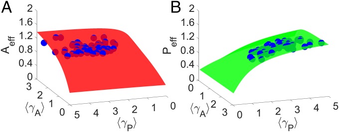
Does our reduced 2D system capture some basic properties of real bipartite mutualistic networks? Treating the effective mutualistic interaction strengths ($⟨{\gamma }_P⟩$ and $⟨{\gamma }_A⟩$) as two independent parameters in the reduced model, we calculate the effective pollinator and plant abundances for each pair of the parameters. In the 3D plot of an effective species abundance vs. $⟨{\gamma }_P⟩$ and $⟨{\gamma }_A⟩$, we obtain a surface as shown in Fig. 1A for the pollinator and in Fig. 1B for the plant. We can then calculate, for each real network, the parameters $⟨{\gamma }_P⟩$ and $⟨{\gamma }_A⟩$ as well as the average pollinator and plant abundances, generating a data point in each case. For the reduced model to be a reasonable representation of the real network, the point must be close to the corresponding smooth 2D surface. As shown in Fig. 1, the data points from all 59 empirical real world networks (SI Appendix, Table S1) are near the corresponding surfaces from the reduced model, providing preliminary evidence that the reduced model captures the essential behavior of the real networks from a wide geographical range across continents and climatic zones. As we will show, however, the detailed averaging process can play a role in the model’s predictive power of the average abundances and the tipping point.

Fig. 1.

Validity test of the reduced model in terms of the average pollinator and plant abundances. In the 3D plot of an average species abundance vs. the two average mutualistic interaction strengths, which are regarded as two independent parameters, the reduced 2D model generates a surface for (A) pollinator (red) and (B) plant (green) abundances. The blue dots are the corresponding data points representing the stable steady states calculated from $59$ real world networks. For each network, the parameter values of $⟨{\gamma }_A⟩$ and $⟨{\gamma }_P⟩$ are calculated by an unweighted average. Other parameters are $h=0.7$, $t=0.5$, ${\beta }_{ii}^{(A)}={\beta }_{ii}^{(P)}=1$, ${\alpha }_i^{(A)}={\alpha }_i^{(P)}=0.3$, ${\mu }_A={\mu }_P=0.0001$, and ${\gamma }_0=1$. The data points from all 59 real networks are in the vicinity of the respective smooth surfaces from the 2D reduced system, providing preliminary validity support.

Reducing the high-dimensional system (i) to the effective 2D system (iii) entails an inevitable loss of detailed information about the original system. However, since predicting the occurrence of the tipping point through the system resilience function is our goal, the primary question is whether the reduced 2D system has predictive power, despite the loss of certain details about the dynamical evolution of the original system. In the following, we present strong evidence that the answer to this question is affirmative.

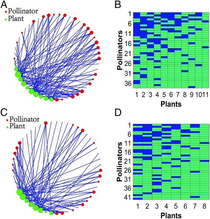
A resilience function is a relationship between the average species abundance and some parameter with variations that reflect the impact on the environment caused by, for example, global warming or direct human activities, such as overuse of pesticides (21–23), where a larger impact corresponds to a higher value of the parameter. Since pollinators are more vulnerable to environmental changes than plants, we focus on two parameters: (i) $f_n$—the fraction of pollinators that have become extinct because of environmental deterioration and (ii) $\kappa$—the average pollinator decay rate. From the standpoint of plants, the disappearance of a specific pollinator means the loss of a number of links, as any pollinator typically interacts with several plants. Thus, we will also consider the parameter $f_l$, the fraction of links destroyed as a result of the death of a fraction $f_n$ of pollinators. With respect to $\kappa$, we note that the parameter ${\kappa }_i$ in the original system (i) characterizes the pollinator decay caused by a decrease in the pollinator growth rate and/or an increase in the pollinator mortality rate. Continuous deterioration of the environment leads to a gradual increase in the average decay rate $\kappa$. While we have studied all 59 mutualistic networks derived from real data, we report the detailed validation results from 2 representative networks: network $A$ obtained from data recorded at Tenerife, Canary Islands (24) and network $B$ from an empirical study at Hestehaven, Denmark (25). Network $A$ has 38 pollinators and 11 plants, and there are 106 mutualistic interactions. Network $B$ has 42 pollinators and eight plants, with 79 mutualistic interactions. The structures of the two networks are shown in Fig. 2 A and C, respectively, whereas their matrix representations are shown in Fig. 2 B and D, respectively.

Fig. 2.

Network structure of two empirical mutualistic networks from real data. A and B correspond to network $A$. C and D correspond to network $B$. The plants in A and C are marked as green, while the pollinators are marked as red. B and D are the matrix representations of networks $A$ and $B$, respectively. The blue blocks indicate that the corresponding pollinator and plant have a mutualistic connection. Column and row numbers correspond to individual plant and pollinator species. Species are ordered according to their number of interactions.

Resilience Functions in Systems Without a Tipping Point.

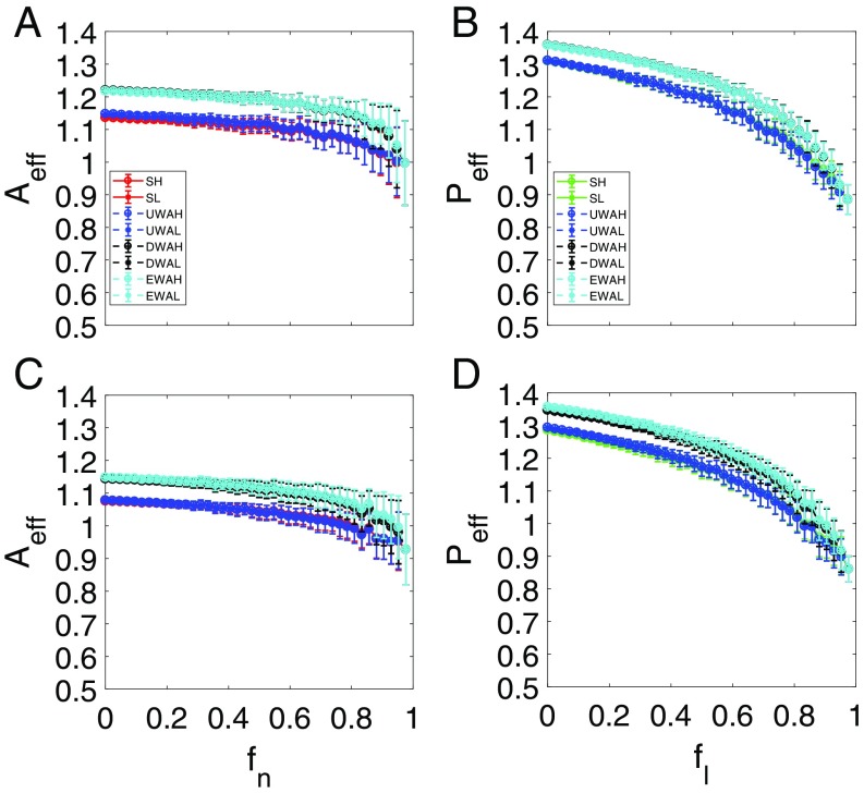
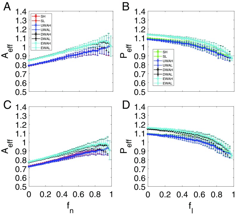
We first examine the case where the system does not exhibit any tipping point. For each value of $f_n$, there are many possible network structures, rendering necessary a description based on statistical ensemble averaging. (Representative individual resilience functions are shown in SI Appendix, Fig. S1.) Fig. 3A shows, for network $A$, four types of pollinator abundances vs. $f_n$ (each with 100 statistical realizations): one from the original network (Fig. 3A, red) and three from the reduced model with different averaging methods (Fig. 3A, blue, black, and cyan corresponding to averaging methods i–iii, respectively). We see that averaging method i leads to abundance variations that are in good agreement with those from the original network, while systematic deviations exist for the results from averaging methods ii and iii, although they agree with each other. Fig. 3B shows, for network $A$, the corresponding plant abundance vs. $f_l$, where the results from the original network are displayed in Fig. 3B, green. The averaging process i leads again to average abundance variations in agreement with those from the original network. The results for network $B$ are shown in Fig. 3 C and D. We see that, for both networks in the parameter setting studied, the remaining pollinators and plants never come close to extinction, even when the fraction of removed pollinators approaches one. The reason is precisely mutualistic interactions: even if there is only one remaining pollinator, at least one plant will be connected with this pollinator. Because of the mutualistic interactions, both the pollinator and plant will survive, and the network system does not exhibit a tipping point. In this parameter regime, the small migration rate has no effect on system dynamical features, such as the absence of a tipping point. The main message of this example is that the reduced model is capable of capturing the abundance variation patterns of both pollinators and plants in the original networked systems.

Fig. 3.

Resilient functions without tipping point. For networks $A$ (A and B) and $B$ (C and D), pollinator abundance (A and C) vs. $f_n$, the fraction of removed pollinators, and plant abundance (B and D) vs. $f_l$, the fraction of removed mutualistic links corresponding to the value of $f_n$ in A and C. The red curves in A and C and the green curves in B and D are the average pollinator and plant abundances, respectively, from the original system. The blue, black, and cyan curves in all of the panels are the abundances from the reduced 2D system using averaging methods i–iii, respectively. The circles and asterisks in all panels correspond to cases where the initial abundance values are relatively high (10) and low (0.01), respectively. For each value of $f_n$ (or $f_l$), results from 100 statistical realizations are displayed. The parameters are $h=0.7$, $t=0.5$, ${\beta }_{ii}^{(A)}={\beta }_{ii}^{(P)}=1$, ${\alpha }_i^{(A)}={\alpha }_i^{(P)}=0.3$, ${\mu }_A={\mu }_P=0.0001$, ${\gamma }_0=1$, and $\kappa =0$. The notations SH and SL stand for the high and low initial values of the original average species abundance, respectively. UWAH, UWAL, DWAH, DWAL, EWAH, and EWAL denote unweighted average high, unweighted average low, degree-weighted average high, degree-weighted average low, eigenvalue-weighted average high, and eigenvalue-weighted average low, respectively.

A phenomenon in Fig. 3 is that, as $f_n$ is increased so that more pollinators are removed, the average plant abundance decays faster with $f_l$ than the average pollinator abundance with $f_n$. The reason is that removing one pollinator typically entails removing a number of mutualistic links, which have a more devastating effect on the plant abundance as a whole.

Power of the Reduced Model in Predicting Tipping Points.

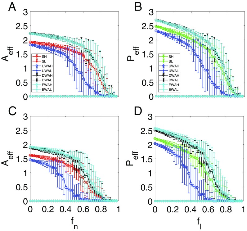
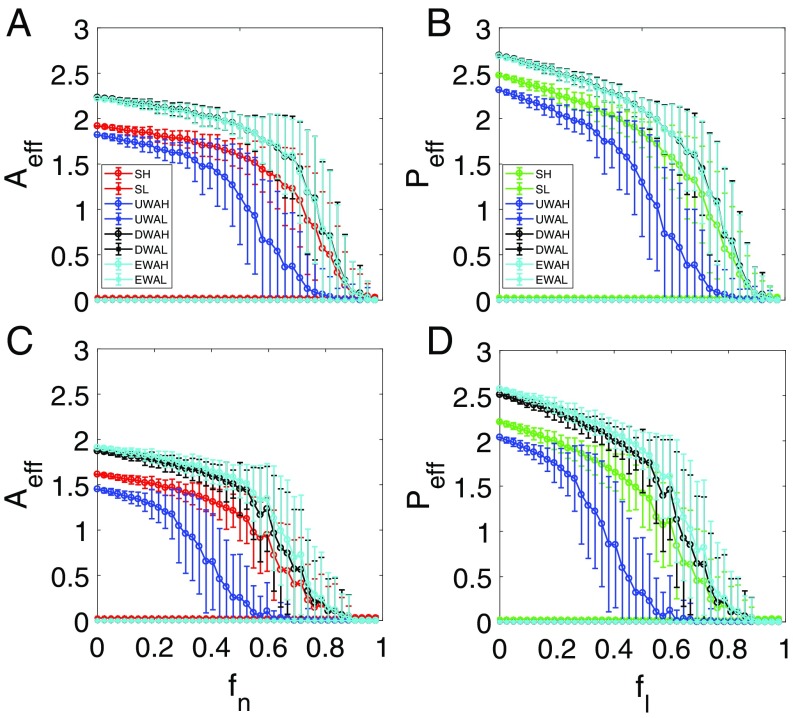
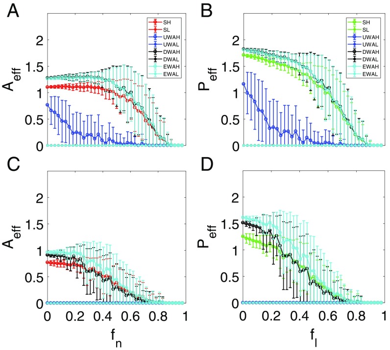
We now consider parameter regimes where the mutualistic network system exhibits a tipping point. An examination of the individual resilience functions (SI Appendix, Fig. S2) for networks $A$ and $B$ reveals that, as $f_n$ for pollinators (or the corresponding $f_l$ for plants) is increased toward unity, there exists a critical point past which the species abundances collapse to almost zero, signifying a tipping point. The corresponding ensemble-averaged resilience functions are shown in Fig. 4. For both networks, the 2D model tends to generate abundance values that deviate from the corresponding true values from the original system. In particular, for the reduced model derived through averaging method i, the abundance values are somewhat smaller than those from the original system, while the opposite behavior occurs for the reduced model with averaging method ii or iii. These deviations are expected, considering the drastic approximations used in deriving the reduced model. While all three types of average in the reduced model generate results indicating the occurrence of a tipping point, a key issue is the accuracy of the predicted parameter value where a tipping point is reached. In particular, if a reduced model does indeed possesses predictive power for the tipping point, it should predict its occurrence at the correct critical point in the original network. In this regard, we see that the reduced model with averaging method i fails to predict the location of the tipping point, whereas the 2D model with averaging method ii or iii yields the true critical point. Since methods ii and iii are based on some sort of weighted averaging process (i.e., with respect to nodal degrees and eigenvectors), the results in Fig. 4 point at the importance of imposing weighted averaging process in the dimension reduction process. This conclusion holds not only for the two networks in Fig. 4 but also, for other networks studied.

Fig. 4.

Resilient functions with a tipping point. For networks $A$ (A and B) and $B$ (C and D), ensemble-averaged pollinator abundance (A and C) vs. $f_n$, the fraction of removed pollinators, and ensemble-averaged plant abundance (B and D) vs. $f_l$, the fraction of removed mutualistic links corresponding to the value of $f_n$ in A and C. The legends are the same as in Fig. 3. The notations SH and SL stand for the high and low initial values of the original average species abundance, respectively. UWAH, UWAL, DWAH, DWAL, EWAH, and EWAL denote unweighted average high, unweighted average low, degree-weighted average high, degree-weighted average low, eigenvalue-weighted average high, and eigenvalue-weighted average low, respectively. The parameters are $h=0.2$, $t=0.5$, ${\beta }_{ii}^{(A)}={\beta }_{ii}^{(P)}=1$, ${\alpha }_i^{(A)}={\alpha }_i^{(P)}=-0.3$, ${\mu }_A={\mu }_P=0.0001$, ${\gamma }_0=1$, and $\kappa =0$. Before $f_n$ (or $f_l$ for plants) reaches unity, a tipping point associated with total collapse of the system occurs at which the species abundances are diminished.

While structural change in the network, such as gradual removal of nodes (pollinators), can trigger a tipping point, there are alternative scenarios, such as parameter changes. Here, we consider the situation where the mutualistic network structure remains intact, but the death rate of the pollinator increases because of environmental deterioration. Specifically, we increase the pollinator decay rate $\kappa$ from zero and calculate the species abundances from the original network and from the three averages of the reduced system. The results are shown in Fig. 5. We see that, similar to the case where the network structure is altered through continuous removal of pollinators (compare with Fig. 4), the reduced model through averaging method ii or iii has a remarkable predictive power for the tipping point in that the predicted critical value of $\kappa$ at which the species abundances collapse to zero agrees well with that from the original system.

Fig. 5.

Predicting tipping point triggered by an increase in pollinator mortal (decay) rate. For networks $A$ (A and B) and $B$ (C and D), resilience functions exhibit a tipping point as the pollinator decay rate $\kappa$ is continuously increased. The red and green curves are the average pollinator (A and C) and plant (B and D) abundances from the original networks, while the blue, black, and cyan curves in all of the panels are the results from the reduced system using averaging methods i–iii, respectively. The parameters are $h=0.6$, $t=0.5$, ${\beta }_{ii}^{(A)}={\beta }_{ii}^{(P)}=1$, ${\alpha }_i^{(A)}={\alpha }_i^{(P)}=0.3$, ${\mu }_A={\mu }_P=0.0001$, and ${\gamma }_0=1$. Note that the network structure remains intact, as no pollinator is removed. As for the case of removing pollinators, the reduced system with averaging method ii or iii is able to predict the onset of the tipping point correctly. Note the occurrence of a hysteresis behavior (predicted by our mathematical analysis).

In our computations, we set a relatively small value for the migration rate for all pollinator species: $\mu =0.0001$—the same value used in previous studies (13, 20). We find that changing this value in a small range has no effect on the tipping point dynamics. Especially before the occurrence of a tipping point, the species abundances are high, so that the changes caused by migration are negligible. After the tipping point, the injection of a small number of species will not be able to restore the abundances on the network scale.

Role of Network Randomness in the Reduced Model.

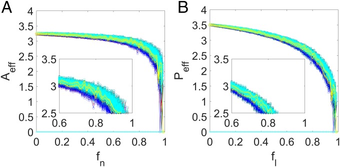
Our extensive computations of the large number of empirical mutualistic networks indicate that a 2D reduced system obtained through degree- or eigenvector-weighted average can correctly predict the tipping point, while the reduced system with unweighted averaging fails to do so. One plausible reason is the lack of sufficient randomness in the network structure. In fact, despite the large variations in their size and structure, the real networks are not quite as random. For a purely random network, either unweighted or weighted averaging has the same effect on the reduced model. To test this proposition and to further show the importance of weighted averaging in the dimension reduction process for real networks, we study artificial random mutualistic networks. Concretely, we construct an ensemble of model networks of $80$ pollinators and $40$ plants with $960$ mutualistic links randomly distributed between the pollinators and the plants and obtain a 2D system through the three averaging processes. As shown in Fig. 6, not only are the three averaging processes able to predict accurately the tipping point, but the differences between the effective abundances that they produced and the actual abundance are small.

Fig. 6.

Reduced system for purely random mutualistic networks. For an ensemble of artificial networks with $80$ pollinators, $40$ plants, and $960$ completely randomly distributed mutualistic links, (A) the average pollinator abundance vs. $f_n$ and (B) the average plant abundance vs. the corresponding parameter $f_l$. In both panels, four types of average abundances are displayed: one from the original network (the red curve in A and the green curve in B) and three from the reduced model. In particular, the blue, black, and cyan traces in both panels are the effective abundances from the reduced model with unweighted, degree-weighted, and eigenvector-weighted averaging, respectively. The circles and asterisks curves in both panels indicate the cases where the initial species abundance is high (10) or low (0.01), respectively. The yellow curves represent the individual realizations for the original system and three types of reduced systems. For each value of $f_n$ (or equivalently, $f_l$), 100 network realizations are used. The parameters are $h=0.4$, $t=0.5$, ${\beta }_{ii}^{(A)}={\beta }_{ii}^{(P)}=1$, ${\alpha }_i^{(A)}={\alpha }_i^{(P)}=-0.3$, ${\mu }_A={\mu }_P=0.0001$, and ${\gamma }_0=1$. The remarkable feature is that, if the original mutualistic network is random, all three types of reduced model can predict correctly the tipping point, regardless of the specific averaging process used in deriving the model. The key message is that the failure of the reduced model through unweighted averaging can be attributed to the lack of sufficient randomness in the real mutualistic networks.

Robust Predictive Power of the Reduced Model Against Stochastic Disturbances (Noises).

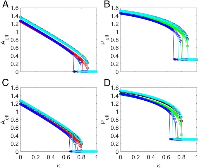
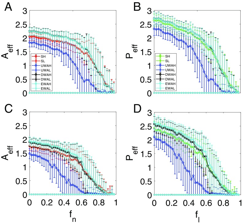
Is our reduced model capable of predicting the tipping point when stochastic disturbances are present in the original network? To address this question, we test the predictive power of the reduced model by considering stochastic abundance and parameter fluctuations. First, we assume that there is additive, independent white Gaussian noise in the dynamic equation for the abundance of each species. The results are shown in Fig. 7, where the color legends are the same as those in Fig. 3. We see that, despite the additive noise, the reduced model still predicts correctly the tipping point, where the performance of the model derived using the degree- and eigenvalue-averaging methods is better than that of the model based on unweighted averaging. Second, we study the case where there is randomness in the intraspecific competition rate as motivated by the consideration that, in reality, the intensity of intraspecific competition varies from one species to another. The results are shown in Fig. 8. We see that, despite the large variations in the species abundances caused by the parameter perturbation, the reduced model based on a weighted average method (averaging method ii or iii) is still capable of predicting the correct tipping point as in Fig. 4.

Fig. 7.

Predictive power of reduced model in the presence of noise. For networks $A$ (A and B) and $B$ (C and D), ensemble-averaged pollinator abundance (A and C) vs. $f_n$ and ensemble-averaged plant abundance (B and D) vs. $f_l$. The legends are the same as in Fig. 3. The notions SH and SL stand for values of the original average species abundance, respectively. UWAH, UWAL, DWAH, DWAL, EWAH, and EWAL denote unweighted average high, unweighted average low, degree-weighted average high, degree-weighted average low, eigenvalue-weighted average high, and eigenvalue-weighted average low, respectively. The parameters are $h=0.2$, $t=0.5$, ${\beta }_{ii}^{(A)}={\beta }_{ii}^{(P)}=1$, ${\alpha }_i^{(A)}={\alpha }_i^{(P)}=-0.3$, ${\mu }_A={\mu }_P=0.0001$, ${\gamma }_0=1$, and $\kappa =0$. Independent white Gaussian noises of strength 0.1 are added to the full evolutionary equations of the species.

Fig. 8.

Robustness of reduced model under random parameter fluctuations. For networks $A$ (A and B) and $B$ (C and D), ensemble-averaged pollinator abundance (A and C) vs. $f_n$ and ensemble-averaged plant abundance (B and D) vs. $f_l$. The legends are the same as in Fig. 3. The notions SH and SL stand values of the original average species abundance, respectively. UWAH, UWAL, DWAH, DWAL, EWAH, and EWAL denote unweighted average high, unweighted average low, degree-weighted average high, degree-weighted average low, eigenvalue-weighted average high, and eigenvalue-weighted average low, respectively. The parameters are $h=0.2$, $t=0.5$, ${\alpha }_i^{(A)}={\alpha }_i^{(P)}=-0.3$, ${\mu }_A={\mu }_P={10}^{-4}$, ${\gamma }_0=1.0$, and $\kappa =0$. Random parameter fluctuations occur in the intraspecific competition rates: ${\beta }_{ii}^{(A)}={\beta }_{ii}^{(P)}\in U(0.7,1.3)$, where $U$ stands for uniform distribution.

Effects of Interspecific Competition.

So far, we have neglected interspecific competitions, as they are generally much weaker than intraspecific competition. Mathematically, interspecific interactions can be modeled through nonzero off-diagonal elements in the competition matrices ${\beta }^P$ and ${\beta }^A$ in Eq. 1, which change the structures of these matrices. It is thus useful to investigate the effects of interspecific competition. Our computations reveal that the 2D reduced model captures all essential features of the mutualistic networked systems, even in the presence of interspecific competition, as shown in Figs. 9 and 10, for the cases where tipping points are absent and present, respectively.

Fig. 9.

Effect of interspecific competition on species abundance in the absence of a tipping point. For networks $A$ (A and B) and $B$ (C and D), ensemble-averaged pollinator abundance (A and C) vs. $f_n$ and ensemble-averaged plant abundance (B and D) vs. $f_l$. The legends are the same as in Fig. 3. The notions SH and SL stand for the high and low initial values of the original average species abundance, respectively. UWAH, UWAL, DWAH, DWAL, EWAH, and EWAL denote unweighted average high, unweighted average low, degree-weighted average high, degree-weighted average low, eigenvalue-weighted average high, and eigenvalue-weighted average low, respectively. The intraspecific and interspecific competitions are incorporated into the modeled through ${\beta }_{ii}^{(A)}={\beta }_{ii}^{(P)}=1$ and ${\beta }_{ij}^A={\beta }_{ij}^P=0.01$, respectively. The parameters are $h=0.7$, $t=0.5$, ${\alpha }_i^A={\alpha }_i^P=0.3$, ${\mu }_A={\mu }_P={10}^{-4}$, ${\gamma }_0=1.0$, and $\kappa =0$. The interspecific competition reduces the abundances but has no significant effect on their overall trends of variation.

Fig. 10.

Effect of interspecific competition on tipping point dynamics. For networks $A$ (A and B) and $B$ (C and D), ensemble-averaged pollinator abundance (A and C) vs. $f_n$ and ensemble-averaged plant abundance (B and D) vs. $f_l$. The intraspecific and interspecific competitions are incorporated into the model the same way as in Fig. 9. The parameters are $h=0.2$, $t=0.5$, ${\alpha }_i^{(A)}={\alpha }_i^{(P)}=-0.3$, ${\mu }_A={\mu }_P={10}^{-4}$, ${\gamma }_0=1.0$, and $\kappa =0$. While interspecific competition somewhat reduces the species abundances, the emergence of the tipping point is not affected.

Fig. 9 is obtained under the same setting as that of Fig. 3, except that interspecific competition is now included. Comparing Fig. 9 with Fig. 3, we see that the competition results in somewhat lower pollinator and plant abundance, which is intuitive. For small values of $f_n$, the number of pollinators is large, and therefore, the interspecific competition among the pollinators is relatively strong. In this case, the species abundances are markedly lower than the corresponding values in the absence of interspecific competition. As $f_n$ is increased, the number of species is reduced, resulting in increasingly weak interspecific competition and consequently, smaller reductions in the abundances. As the strength ${\beta }_{ij}$ of the interspecific competitive interaction is increased, simulations of both the original networked and the 2D reduced systems give lower species abundances. The remarkable feature is that, when interspecific competition is taken into account, the 2D reduced system can still reliably predict the species abundances, with the unweighted averaging scheme giving the best result, while the degree- and eigenvector-weighted schemes predict correctly the trend of the abundance variations.

Fig. 10 shows the effects of interspecific competition in the parameter regime where there is a tipping point. Comparing Fig. 10 with Fig. 4, we see that, with the inclusion of interspecific competition, the 2D reduced model derived from the degree- or eigenvector-weighting scheme predicts the tipping point accurately, which is similar to the case where such competition is absent. The mere effect of a reasonable amount of interspecific competition is simply reduced abundances. (For sufficiently large values of the interspecific interaction strength, both the original and the reduced 2D models agreeably give the result of species extinction.)

Occurrence of a Tipping Point in the 2D Parameter Space.

Both structural change (removal of certain pollinator species) and parameter change (increase in $\kappa$) can lead to a tipping point. It is useful to examine the occurrence of a tipping point in the 2D parameter space $(f_n,\kappa )$, as both types of changes can be expected in realistic systems (21). We calculate the critical parameter value for the tipping point through both the original system and the reduced model. A representative result for network $A$ is shown in SI Appendix, Fig. S3 for $\kappa \in [0,0.64]$ and $f_n\in [0,0.974]$. (The corresponding result for network $B$ is presented in Fig. S4.) The general observation is that, while there are variations in the location of the tipping point in the $f_n$ direction, the location variations in the $\kappa$ direction are relatively smooth. In fact, our reduced model incorporating either the degree- or the eigenvector-averaging method gives an accurate prediction of the tipping point in the parameter plane.

A Mathematical Analysis of the System Dynamics with an Explanation of the Emergence of a Tipping Point.

The 2D reduced model provides mathematical insights into the emergence of a tipping point. The relevant quantities are the steady-state values of the species abundances. Setting $d{P}_{eff}/dt=0$ and $d{A}_{eff}/dt=0$, we can obtain the algebraic equations for the steady-state solutions (SI Appendix, Note 3).

We first consider the parameter regime in which the system does not exhibit a tipping point (e.g., Figs. 1 and 3). In this case, we have $\alpha >0$, and the physically meaningful steady-state solutions are given by

$$\begin{array}{c}P\prime \approx \frac{1}{\beta }\left[\alpha +\frac{⟨{\gamma }_P⟩A\prime }{1+h⟨{\gamma }_P⟩A\prime }\right],\\ A\prime \approx \frac{1}{\beta }\left[\alpha -\kappa +\frac{⟨{\gamma }_A⟩P\prime }{1+h⟨{\gamma }_A⟩P\prime }\right].\end{array}$$ [4]

The solutions of Eq. 4 can be conveniently expressed in terms of the following algebraic equation for $A\prime$:

$$q_1{A}^{\prime 2}+q_{2}A\prime +q_3=0,$$ [5]

where the coefficients $q_1$, $q_2$, and $q_3$ are given by

$$\begin{array}{c}{q}_1\equiv -(h⟨{\gamma }_P⟩+h⟨{\gamma }_A⟩⟨{\gamma }_P⟩+h^2\alpha ⟨{\gamma }_A⟩⟨{\gamma }_P⟩),\\ q_2\equiv -{\beta }^2-h\alpha \beta ⟨{\gamma }_A⟩+h\alpha \beta ⟨{\gamma }_P⟩+⟨{\gamma }_A⟩⟨{\gamma }_P⟩,+2h\alpha ⟨{\gamma }_A⟩⟨{\gamma }_P⟩+h^2{\alpha }^2⟨{\gamma }_A⟩⟨{\gamma }_p⟩-\kappa (h\beta ⟨{\gamma }_P⟩+h⟨{\gamma }_A⟩⟨{\gamma }_P⟩+h^2\alpha ⟨{\gamma }_A⟩⟨{\gamma }_P⟩),\\ q_3\equiv \alpha \beta +\alpha ⟨{\gamma }_A⟩+h{\alpha }^2⟨{\gamma }_A⟩-\kappa (\beta +h\alpha ⟨{\gamma }_A⟩).\end{array}$$

For $\kappa =0$, we have $q_1<0$ and $q_3>0$. Of the two solutions of Eq. 5, one is positive, and another is negative. The abundance values of $A\prime$ in Figs. 1 and 3 are then approximately the value of the positive solution.

We next consider the parameter regime, in which the mutualistic system exhibits a tipping point (Fig. 4) (i.e., $\alpha <0$). For $\kappa =0$, from the stability analysis in SI Appendix, Note 3 for an initial state with high abundances, we have $\alpha +(⟨{\gamma }_P⟩)A\prime /(1+h⟨{\gamma }_P⟩A\prime )>0$ and $\alpha -\kappa +(⟨{\gamma }_A⟩P\prime )/(1+h⟨{\gamma }_A⟩P\prime )>0$ in the parameter region where the abundance values are large (i.e., before the tipping point). In this case, the steady-state solutions are given by SI Appendix, Eqs. S14 and S16. After the tipping point has been reached, the steady-state solutions are given by SI Appendix, Eqs. S15 and S17. In this case, the physically meaningful solutions are $A\prime \approxeq \mu$ and $P\prime \approxeq \mu$, which correspond to the extinction state. The mathematical conditions under which the tipping point occurs are thus $q_2^2-q_1{q}_3=0$. In general, the occurrence of a tipping point is caused by the changes in the quantities $⟨{\gamma }_A⟩$ and $⟨{\gamma }_P⟩$.

For a tipping point induced by an increase in the species decay rate $\kappa$ (Fig. 5), we have $\alpha >0$. Before the tipping point, the value of $\kappa$ is small, and we have $\alpha -\kappa +(⟨{\gamma }_A⟩P\prime )/(1+h⟨{\gamma }_A⟩P\prime )>0$ and $\alpha +(⟨{\gamma }_P⟩A\prime )/(1+h⟨{\gamma }_P⟩A\prime )>0$. In this case, we can obtain the approximate steady-state solution from Eq. 5. For larger values of $\kappa$, the solutions of Eq. 5 become complex, which are physically unrealistic. The condition for the onset of complex solutions is $q_2^2-4q_1{q}_3<0$. The approximate critical value ${\kappa }_{C1}$ for the occurrence of the tipping point can then be calculated from the relation $q_2^2-4q_1{q}_3=0$. However, there exists another critical value, denoted as ${\kappa }_{C2}$, which can be seen as follows.

As the value of $\kappa$ approaches ${\kappa }_{C2}$, the following inequality holds: $\alpha -\kappa +(⟨{\gamma }_A⟩P\prime )/(1+h⟨{\gamma }_A⟩P\prime )<0$, under which the steady-state solutions are given by SI Appendix, Eqs. S14 and S17. In particular, we have

$$\begin{array}{c}P\prime \approx \frac{1}{\beta }\left[\alpha +\frac{⟨{\gamma }_P⟩A\prime }{1+h⟨{\gamma }_P⟩A\prime }\right]\hspace{0.17em}\text{and}\\ A\prime \approx \mu .\end{array}$$

Since $\mu \ll 1$, we have $P\prime \approx \alpha$. The critical value of $\kappa$ for the emergence of this steady state can be obtained from

$$\alpha -{\kappa }_{C2}+\frac{⟨{\gamma }_A⟩P\prime }{1+h⟨{\gamma }_A⟩P\prime }=0.$$

The value of ${\kappa }_{C1}$ is typically larger than that of ${\kappa }_{C2}$, which gives an interval of $\kappa$, in which the system exhibits bistability or a hysteresis behavior, as shown in Fig. 5.

Overall, the 2D reduced model thus provides a mathematical paradigm by which a number of distinct dynamical phenomena in mutualistic interacting networks can be understood. For example, as pollinators are removed one after another from the system (i.e., as $f_n$ is gradually increased), for $\alpha <0$, the quantities $⟨{\gamma }_A⟩$ and $⟨{\gamma }_P⟩$ change in such a way that the system exhibits a tipping point without any hysteresis behavior. However, as the species decays faster (i.e., as the value of $\kappa$ is increased), a hysteresis can arise. While the value of $h$ can affect the critical parameter values and abundances, it has little effect on the occurrence of a tipping point.

The analysis leads to insights into the effect of varying the value of the parameter $h$, the half-saturation constant. The reason that we choose different values of $h$ for different parameter setting is to ensure that the system exhibits a tipping point as the value of $\kappa$ or $f$ is varied. From the mathematical analysis, for cases where a tipping point occurs, $h$ will affect the critical values of $\kappa$, $⟨{\gamma }_A⟩$, and $⟨{\gamma }_P⟩$, whereas varying $f_n$ can cause the values of $⟨{\gamma }_A⟩$ and $⟨{\gamma }_P⟩$ to change. From a mathematical standpoint, the type of mutual interactions in our model belongs to Holling type II (26, 27). From an ecological point of view, the half-saturation constant $h$ characterizes the relaxation time of the species after each mutual interaction, with strength that is described by the parameter $\gamma$. The effect of varying $h$ on the system dynamics is thus characteristically different from those caused by variations in $\kappa$ and $f$.

Discussion

Complex dynamical systems exhibiting a tipping point are widespread, and it is of interest to understand the dynamical mechanism of the tipping point and to develop predictive tools. To accomplish these goals, a viable solution is dimension reduction. We focus in this paper on bipartite mutualistic networks, not only as a concrete example to show the use of dimension reduction but also, because of the fundamental values of safeguarding pollinators to human survivability (28). In a mutualistic network system, a tipping point typically exists. As the environment continues to deteriorate, the system can drift toward the tipping point, where the catastrophic phenomenon of pollinator collapse will occur. The backbone that supports the functioning of such a network is mutualistic interactions between the pollinators and plants. To understand the role of the interactions with respect to the emergence of a tipping point, both species of the bipartite network must be retained in a reduced model. That is, the minimum dimension of the reduced system should be two [a 1D reduced model (18) is inadequate to describe mutualistic interactions]. With this in mind, we carry out a dimension reduction process by resorting to different types of averaging methods for species abundances. In particular, given an empirical mutualistic network, we carry out averaging processes to arrive at a 2D model with two collective dynamical variables: one for the pollinators and another for the plants. The average can be either unweighted or weighted. We show that our 2D reduced model captures the essential features of all 59 available real world mutualistic networks, not only in terms of the average abundances but more importantly, in terms of the occurrence of the tipping point, even in the presence of stochastic disturbances. We also find that, because of the lack of sufficient randomness in real mutualistic networks, a weighted average (e.g., based on degrees or eigenvectors) is necessary for the reduced model to exhibit a tipping point at the same critical parameter value as with the original network. Our 2D model can thus serve as a generic paradigm for understanding the tipping point dynamics in real world mutualistic networks. For example, the 2D model can be exploited to investigate a variety of nonlinear dynamical phenomena in mutualistically interacting networked systems, such as bifurcations (29), basin structures (30, 31), crises (32), and transient chaos (33–38), which would otherwise be infeasible with the original systems because of their high dimensionality.

References

- 1.Gladwell M. The Tipping Point: How Little Things Can Make a Big Difference. Little, Brown and Company; New York: 2000. [Google Scholar]
- 2.Scheffer M, et al. Early-warning signals for critical transitions. Nature. 2009;461:53–59. doi: 10.1038/nature08227. [DOI] [PubMed] [Google Scholar]
- 3.Veraart AJ, et al. Recovery rates reflect distance to a tipping point in a living system. Nature. 2012;481:357–359. doi: 10.1038/nature10723. [DOI] [PubMed] [Google Scholar]
- 4.Ashwin P, Wieczorek S, Vitolo R, Cox P. Tipping points in open systems: Bifurcation, noise-induced and rate-dependent examples in the climate system. Philos Trans A Math Phys Eng Sci. 2012;370:1166–1184. doi: 10.1098/rsta.2011.0306. [DOI] [PubMed] [Google Scholar]
- 5.Lenton TM, Livina VN, Dakos V, van Nes EH, Scheffer M. Early warning of climate tipping points from critical slowing down: Comparing methods to improve robustness. Philos Trans A Math Phys Eng Sci. 2012;370:1185–1204. doi: 10.1098/rsta.2011.0304. [DOI] [PMC free article] [PubMed] [Google Scholar]
- 6.Boettiger C, Hastings A. Tipping points: From patterns to predictions. Nature. 2013;493:157–158. doi: 10.1038/493157a. [DOI] [PubMed] [Google Scholar]
- 7.Lontzek TS, Cai YY, Judd KL, Lenton TM. Stochastic integrated assessment of climate tipping points indicates the need for strict climate policy. Nat Clim Change. 2015;5:441–444. [Google Scholar]
- 8.Gualdia S, Tarziaa M, Zamponic F, Bouchaudd JP. Tipping points in macroeconomic agent-based models. J Econ Dyn Contr. 2015;50:29–61. [Google Scholar]
- 9.Rahmstorf S. Ocean circulation and climate during the past 120,000 years. Nature. 2002;419:207–214. doi: 10.1038/nature01090. [DOI] [PubMed] [Google Scholar]
- 10.Drake JM, Griffen BD. Early warning signals of extinction in deteriorating environments. Nature. 2010;467:456–459. doi: 10.1038/nature09389. [DOI] [PubMed] [Google Scholar]
- 11.Dai L, Vorselen D, Korolev KS, Gore J. Generic indicators for loss of resilience before a tipping point leading to population collapse. Science. 2012;336:1175–1177. doi: 10.1126/science.1219805. [DOI] [PubMed] [Google Scholar]
- 12.Tylianakis JM, Coux C. Tipping points in ecological networks. Trends Plant Sci. 2014;19:281–283. doi: 10.1016/j.tplants.2014.03.006. [DOI] [PubMed] [Google Scholar]
- 13.Lever JJ, Nes EH, Scheffer M, Bascompte J. The sudden collapse of pollinator communities. Ecol Lett. 2014;17:350–359. doi: 10.1111/ele.12236. [DOI] [PubMed] [Google Scholar]
- 14.Scheffer M. Ecology of Shallow Lakes. Springer Science & Business Media; Berlin: 2004. [Google Scholar]
- 15.Iwasa Y, Andreasen V, Levin S. Aggregation in model ecosystems I. Perfect aggregation. Ecol Model. 1987;37:287–302. [Google Scholar]
- 16.Iwasa Y, Levin S, Andreasen V. Aggregation in model ecosystems II. Approximate aggregation. Math Med Biol. 1989;6:1–23. [Google Scholar]
- 17.Lorenz EN. Deterministic nonperiodic flow. J Atmos Sci. 1963;20:130–141. [Google Scholar]
- 18.Gao J, Barzel B, Barabási AL. Universal resilience patterns in complex networks. Nature. 2016;530:307–312. doi: 10.1038/nature16948. [DOI] [PubMed] [Google Scholar]
- 19.Rohr RP, Saavedra S, Bascompte J. On the structural stability of mutualistic systems. Science. 2014;345:1253497. doi: 10.1126/science.1253497. [DOI] [PubMed] [Google Scholar]
- 20.Dakos V, Bascompte J. Critical slowing down as early warning for the onset of collapse in mutualistic communities. Proc Natl Acad Sci USA. 2014;111:17546–17551. doi: 10.1073/pnas.1406326111. [DOI] [PMC free article] [PubMed] [Google Scholar]
- 21.Goulson D, Nicholls E, Botías C, Rotheray EL. Bee declines driven by combined stress from parasites, pesticides, and lack of flowers. Science. 2015;347:1255957. doi: 10.1126/science.1255957. [DOI] [PubMed] [Google Scholar]
- 22.Kerr JT, et al. Climate change impacts on bumblebees converge across continents. Science. 2015;349:177–180. doi: 10.1126/science.aaa7031. [DOI] [PubMed] [Google Scholar]
- 23.Koh I, et al. Modeling the status, trends, and impacts of wild bee abundance in the United States. Proc Natl Acad Sci USA. 2016;113:140–145. doi: 10.1073/pnas.1517685113. [DOI] [PMC free article] [PubMed] [Google Scholar]
- 24.Dupont YL, Hansen DM, Olesen JM. Structure of a plant–flower-visitor network in the high-altitude sub-alpine desert of Tenerife, Canary Islands. Ecography. 2003;26:301–310. [Google Scholar]
- 25.Montero AC. 2005. The ecology of three pollination networks. Master’s thesis (Aarhus Univ, Aarhus, Denmark)
- 26.Holling CS. Some characteristics of simple types of predation and parasitism. Can Entomol. 1959;91:385–398. [Google Scholar]
- 27.Dale BW, Adams LG, Bowyer RT. Functional response of wolves preying on barren-ground caribou in a multiple-prey ecosystem. J Anim Ecol. 1994;63:644–652. [Google Scholar]
- 28.Potts SG, et al. Safeguarding pollinators and their values to human well-being. Nature. 2016;540:220–229. doi: 10.1038/nature20588. [DOI] [PubMed] [Google Scholar]
- 29.Ott E. Chaos in Dynamical Systems. 2nd Ed Cambridge Univ Press; Cambridge, UK: 2002. [Google Scholar]
- 30.Grebogi C, McDonald SW, Ott E, Yorke JA. Final state sensitivity: An obstruction to predictability. Phys Lett A. 1983;99:415–418. [Google Scholar]
- 31.McDonald SW, Grebogi C, Ott E, Yorke JA. Fractal basin boundaries. Physica D. 1985;17:125–153. [Google Scholar]
- 32.Grebogi C, Ott E, Yorke JA. Crises, sudden changes in chaotic attractors and chaotic transients. Physica D. 1983;7:181–200. [Google Scholar]
- 33.Hastings A, Higgins K. Persistence of transients in spatially structured ecological models. Science. 1994;263:1133–1136. doi: 10.1126/science.263.5150.1133. [DOI] [PubMed] [Google Scholar]
- 34.Hastings A. Transient dynamics and persistence of ecological systems. Ecol Lett. 2001;4:215–220. [Google Scholar]
- 35.Hastings A. Transients: The key to long-term ecological understanding? Trends Ecol Evol. 2004;19:39–45. doi: 10.1016/j.tree.2003.09.007. [DOI] [PubMed] [Google Scholar]
- 36.Hastings A. Timescales, dynamics, and ecological understanding. Ecology. 2010;91:3471–3480. doi: 10.1890/10-0776.1. [DOI] [PubMed] [Google Scholar]
- 37.Hastings A. Timescales and the management of ecological systems. Proc Natl Acad Sci USA. 2016;113:14568–14573. doi: 10.1073/pnas.1604974113. [DOI] [PMC free article] [PubMed] [Google Scholar]
- 38.Lai YC, Tél T. Transient Chaos—Complex Dynamics on Finite-Time Scales. 1st Ed Springer; New York: 2011. [Google Scholar]
Associated Data
This section collects any data citations, data availability statements, or supplementary materials included in this article.