Abstract
Human body motion analysis based on wearable inertial measurement units (IMUs) receives a lot of attention from both the research community and the and industrial community. This is due to the significant role in, for instance, mobile health systems, sports and human computer interaction. In sensor based activity recognition, one of the major issues for obtaining reliable results is the sensor placement/assignment on the body. For inertial motion capture (joint kinematics estimation) and analysis, the IMU-to-segment (I2S) assignment and alignment are central issues to obtain biomechanical joint angles. Existing approaches for I2S assignment usually rely on hand crafted features and shallow classification approaches (e.g., support vector machines), with no agreement regarding the most suitable features for the assignment task. Moreover, estimating the complete orientation alignment of an IMU relative to the segment it is attached to using a machine learning approach has not been shown in literature so far. This is likely due to the high amount of training data that have to be recorded to suitably represent possible IMU alignment variations. In this work, we propose online approaches for solving the assignment and alignment tasks for an arbitrary amount of IMUs with respect to a biomechanical lower body model using a deep learning architecture and windows of 128 gyroscope and accelerometer data samples. For this, we combine convolutional neural networks (CNNs) for local filter learning with long-short-term memory (LSTM) recurrent networks as well as generalized recurrent units (GRUs) for learning time dynamic features. The assignment task is casted as a classification problem, while the alignment task is casted as a regression problem. In this framework, we demonstrate the feasibility of augmenting a limited amount of real IMU training data with simulated alignment variations and IMU data for improving the recognition/estimation accuracies. With the proposed approaches and final models we achieved 98.57% average accuracy over all segments for the I2S assignment task (100% when excluding left/right switches) and an average median angle error over all segments and axes of ° for the I2S alignment task.
Keywords: inertial sensors, automatic sensor placement, automatic sensor alignment, neural networks, deep learning, LSTM, CNN
1. Introduction
Inertial measurement units (IMUs) comprise accelerometers and gyroscopes providing measurements of 3D acceleration including acceleration due to gravity and 3D angular velocity. In most cases, they also contain magnetometers adding 3D magnetic fields. This is also referred to as MIMUs. Nowadays, IMUs are small in size and can be obtained at low cost. They are thus present in a multitude of devices. They also enjoy a widespread use in many different application areas, where humans wear IMUs on the body or nearby, e.g., inside the clothes. This includes, for instance, mobile health and biomechanics [1,2,3,4,5].
The following sections provide related work for the IMU-to-segment (I2S) assignment and alignment problems, first for human body motion capture, and then for activity recognition. Afterwards, related work is provided for applications with simulated and synthetic data. Finally, our scope and contributions are summarized.
1.1. I2S Assignment and Alignment for Inertial Body Motion Capture
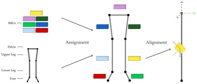
In inertial body motion capture, the data from multiple IMUs, so-called IMU networks, are fused with a biomechanical model of (parts of) the human body to reconstruct segment orientations and joint angles [6,7] and sometimes also joint positions [8]. Figure 1 illustrates a kinematic lower body configuration. For obtaining biomechanical joint angles and positions, both the assignment of each IMU to the respective body segment as well as the position and orientation of each sensor relative to the assigned segment need to be known [7,9,10,11]. The latter is referred to as IMU-to-segment (I2S) alignment or I2S calibration (cf. Figure 1). A comparison of different sensor fusion methods for inertial body motion tracking (segment orientation estimation) regarding I2S alignment errors indicated that the position of the sensor relative to the segment is usually far less important for obtaining valid segment orientations (which are typically of more interest than the positions) than the I2S orientation [7]. Some methods were even shown to be independent of the IMU positioning in this study. In contrast, I2S orientation errors were shown to propagate at least linearly into the orientation estimation of the respective segment (and as a result into the derived joint angles), for all tested methods (without considering joint constraints). Therefore, we focus on I2S assignment and I2S orientation estimation (subsequently denoted I2S alignment) in this work.
Figure 1.
Illustration of the two addressed problems for seven lower body segments and seven IMUs: (i) I2S assignment; and (ii) I2S alignment determination.
Basically, all current I2S calibration procedures assume the I2S assignment to be known. Some approaches estimate an I2S assignment and consider an underlying body model in a hierarchical manner [12,13]. The first used decision trees on manually selected features with correlations of sensor data to subsequently assign 17 IMUs for a full body configuration or eight IMUs for a lower body or trunk configuration during walking trials. The accuracy of this method was between and , if the sensors were on the predefined positions in a suit. If sensors were missing or the positions were altered, the method either did not work or the accuracy decreased considerably ( to ). Another recent approach assigned six IMUs to the lower limbs via constructed decisions based on walking characteristics and a proposed assignment hierarchy [13]. The accuracy of this approach ranged between and after three respectively five seconds of walking. However, the hierarchy needed multiple sensors. In contrast our approach considers each IMU individually and therefore scales to an arbitrary number of IMUs, including, for instance, only one IMU, seven IMUs (one on each considered lower body segment) or more than seven IMUs (multiple IMUs on one segment).
Assuming the I2S assignment to be known, obtaining a correct I2S calibration is still not trivial. Different calibration procedures have been proposed: static pose calibration that requires the user to take on specific poses [10], functional calibration [14,15], which requires the user to perform motions around predefined axes, or technical calibration that requires manual alignment of the IMUs with the bone structure [9]. In [9], typical I2S orientation calibration procedures were validated regarding their accuracy (trueness) and reproducibility (precision) relative to an optical reference system. The accuracy was in the range ° and precision was in the range °. This attests the potentially large (human-induced) errors with respect to (w.r.t.) the I2S orientation, even when persons were instructed to perform the calibration procedure through experts. One recent approach aims at simultaneous joint kinematics and I2S calibration estimation, exploiting moving horizon optimization with additional constraints and priors for the calibration parameters [11].
1.2. I2S Assignment and Alignment for Activity Recognition, Deep Learning Approaches
Besides inertial body motion capture, another related application that is typically based on one or few IMUs, for instance from a mobile phone worn on the body or inside the cloths, is human activity recognition (HAR). Here, the aim is to infer activities, such as walking, sitting or running, from the sensor data. There are many classification approaches that use different manually derived features based on properties of the IMU signals, see, e.g., [16,17]. The classification accuracy largely depends on the feature selection which can be time consuming [18]. This process can also be automated together with the classification model, which leads to end-to-end learning. Here, the resulting model is directly applied to the raw sensor data. Deep learning approaches [19] are a prominent representative for end-to-end learning and have tremendous success in different applications fields, such as computer vision (e.g., image classification, action or gesture recognition [20,21,22,23,24]) or speech recognition [25,26]. There are also related applications to IMU based HAR [18,27], including the recently proposed deep learning framework for HAR. The latter is based on multimodal sensors such as IMUs. It combines local feature learning based on convolutional neural network (CNN) units with time sequence learning based on recurrent long-short-term memory (LSTM) units and is named DeepConvLSTM [18]. Moreover, CNN kernels were analyzed for automatic feature extraction with the aim to transfer these to different HAR domains in order to reduce training time significantly [28]. Our work is inspired by the DeepConvLSTM approach.
One problem for the majority of activity recognition approaches is that many expressive features for the same activity may differ largely, depending on the placement of the IMU relative to the body. For instance the IMU signals in a trouser pocket or at the pelvis are usually different from the signals at the feet in case of walking. This often renders HAR unreliable if the sensor placement is not known. One approach to face this problem is to use features that are robust to location and/or alignment. These are, however, usually less expressive and thus inferior for the recognition of complex motion [29]. In [29] sensor placement variations for wearable activity recognition were investigated in a structured way. The variations where subdivided into: (1) on-body placement (i.e., the place where the user carries the sensor on the body, this corresponds to our I2S assignment); (2) within-body displacements (i.e., the variation of the sensor placement on the respective segment); and (3) orientation (i.e., the device orientation w.r.t. the users body, this corresponds to our I2S orientation alignment). There are also approaches given to mitigate the errors introduced by the respective variations. Wrong on-body placement often renders an activity recognition approach unreliable. A study on optimal positions for HAR was performed in [30]. The within-body displacement can also decrease activity recognition accuracy. Remedy can be found, e.g., by dynamically choosing the most robust features [29,31] or by applying low-pass filtering after orientation correction [32]. Orientation variations yield unreliable rotation dependent features that, however, usually incorporate a lot more information to separate activity classes compared to rotation independent features such as the vector norm [29]. In [33] the effect of 16 IMU orientation variations and different IMU locations to an activity recognition approach was evaluated and severe accuracy decreases were found. A projection of the data to an approximate global frame as well as a model switch for different body locations was proposed for remedy. There are also approaches that classify the approximate location of one sensor [34,35,36,37] during walking and activities of daily living [38]. In [39] the sensor location and activity was jointly classified using sparse signal representation. Another method used accelerometer and gyroscope data to classify different on-body positions [40]. In [41] the orientation of an IMU w.r.t. the hip was classified considering rotations around one axis in 90° steps. The data were then transformed into the corresponding reference frame resulting in increased accuracy. Note, none of the mentioned approaches reconstructed the complete 3D orientation of the IMU relative to the respective body part, i.e., the I2S alignment. Performing this reconstruction has the advantage that the sensor data can always be rotated into the segment coordinate system, no matter how the sensor is oriented. For a data based approach this automatically introduces the challenge of having enough training data for the different possible orientations. The required amount of training data as well as class labels increases exponentially depending on the intended alignment classification accuracy. Therefore, our approach casts the I2S alignment task as a regression problem and makes use of artificial training data from simulated I2S alignment variations.
1.3. Applications with Simulated/Synthetic IMU Data
There are different frameworks for simulating IMU data from IMU trajectories [42,43], the latter, for instance, used recorded optical motion capture data. In the field of inertial body motion tracking, IMU data simulation is often used for evaluating different estimation methods (e.g., [7,8,44]).
In the field of computer vision, synthetic data were used to augment or create training data for increasing classification performance [45,46,47]. A typical challenge is the difference in feature distortions between synthetic and real data, i.e. the synthetic gap [45,47]. One way to face this problem is by using a multichannel autoencoder to learn the mapping between synthetic and real data [47]. A recent work [46] interpreted the learning of a neural network using synthetic data as learning of a proposal distribution generator for approximate inference in the synthetic-data generative model. This interpretation was used to explain model misspecifications that could be shown by only slight data variations, leading to a significant decrease in classification accuracy. The remedy was found by broadening the synthetic generator via adding an elastic displacement field to the synthetic data, which also lead to significant accuracy improvements [48].
Simulated IMU data, however, have not yet been used and investigated as database for deep learning approaches. In particular, the feasibility of transferring models learned on simulated IMU data to real data scenarios, has, to the best of our knowledge, not yet been investigated.
1.4. Contributions and Scope
Given the importance of sensor assignment and alignment determination in multiple areas, an automatic approach would, on the one hand, reduce the influence of human induced errors and, on the other hand, simplify the installation of an IMU system.
The contributions of this paper can be summarized as follows:
We propose real-time capable deep learning approaches to solve the I2S assignment problem via classification and the I2S alignment problem via regression during walking for IMUs mounted on the lower body. The proposed approaches combine automatic feature learning via CNN units with time dynamic features based on two recurrent neural network approaches (LSTM and GRU). Since each IMU is handled individually, the proposed approaches scale to an arbitrary number of IMUs.
We propose and evaluate methods for simulating IMU training data for a variety of I2S alignment orientations during walking using freely available [49] and newly recorded motion capture datasets. This is our approach for counteracting the problem of requiring the recording of exponentially many training data for sufficiently sampling potential I2S alignment variations.
We investigate the performances of the proposed methods and approaches on simulated and real IMU test data, with different proportions of simulated and real IMU data used for training. The experiments show promising performances for both the classification and the regression problem with only a small amount of recorded IMU data (in terms of alignment variations).
In the following, the proposed methods, the datasets and experiments are introduced in Section 2 and Section 3, respectively. The results and a discussion are given in Section 4, and conclusions are drawn in Section 5.
2. Methods
First, the addressed problems are stated in Section 2.1. Then, the proposed network configurations with their different components are explained in Section 2.2. The involved coordinate frames and transformations are formalized in Section 2.3. Finally, Section 2.4 provides details on different aspects of our IMU data simulation.
2.1. Problem Statement
We address the following problems during walking motion (cf. Figure 1):
I2S assignment: Each IMU is separately assigned to the skeleton segment it is attached to. This results in the classification problem of mapping a window of (raw) IMU data to one of the seven classes associated to the lower body segments: (1) LeftFoot; (2) LeftLowerLeg; (3) LeftUpperLeg; (4) Pelvis; (5) RightUpperLeg; (6) RightLowerLeg; and (7) RightFoot.
I2S alignment: Each IMU’s orientation w.r.t. the associated segment is estimated via regression based on a window of IMU data. Note, I2S positions are assumed constant (on the middle of the respective segment) in this work.
In both cases, we use windows of 128 gyroscope and accelerometer data samples of the considered IMU as inputs. Moreover, throughout this work, the windows are always shifted by 16 data samples.
Note, successfully solving the stated problems provides I2S assignment and alignment of, in principle, any number of IMUs (they are treated separately) to the lower body skeleton in about two seconds of walking (assuming 60 Hz frequency) without using magnetometer data.
2.2. Proposed Networks
This section presents the network configurations proposed for solving the above stated problems. It starts with a general overview and then provides a mathematical formalization.
Figure 2 illustrates the structure of the proposed networks for both the classification and the regression task.
Figure 2.
Overview of the proposed network configurations.
The configurations follow the general framework described in [18] with modifications described subsequently. Input denotes the input layer, i.e., (in this work) a window of 128 accelerometer and gyroscope data. Gaussian Noise refers to data augmenting noise samples, which we have introduced for processing simulated IMU data (cf. Section 2.4.1). A regularization based on Input Dropout has been introduced to avoid over-fitting (cf. Section 2.2.4). The main building blocks are the CNN Layer and the RNN Layer, where the latter is constructed differently for the classification and the regression problem. More details including the proposed modifications w.r.t. [18] are provided in Section 2.2.2 and Section 2.2.3. The respective final recurrent layer is densely connected with the output layer Output via a fully connected layer (FC Layer). The output layer either represents classes via probabilities using a Softmax layer (classification problem) or it maps to the components of a vector (regression problem), here representing the I2S alignment orientation. For the former, the class with the highest probability is chosen.
2.2.1. Notation
A deep neural network with layers consists of an input layer with several input units (), several hidden layers with activation units () and an output layer with units . The latter might be a softmax layer for classification or an identity layer mapping to the previous layer for regression.
Given a sequence of T gyroscope () and accelerometer () data of (without loss of generality) one IMU, we stack these data to obtain the input data , where denotes the IMU data at time t. We call the stacked components of the input units () channels.
A dense connection between the input layer () and the next layer at time t (i.e., a fully connected layer) can be formalized as
| (1) |
Here, are the activations of layer 2, and is the weight matrix of layer 1 with the subscript denoting a connection from one activation to another activation. Moreover, represents the weight between activation j in layer 1 and i in layer 2. Further, are the channels of the input data, are the biases and is the non-linear activation function, which is typically applied to each component of the resulting vector separately. The specific functions are given in the subsections below.
2.2.2. Convolutional Neural Network (CNN) Layer
A CNN layer convolves (or often cross-correlates) activations of a layer, e.g., the input layer, with kernels (filters). CNNs with multiple layers perform convolutions on the respective activations of the previous layer. The convolution with the kernel yields a weight sharing between activations, which has different advantages for data with neighborhood relations (either spatially, temporally or both, depending on the kernel used). First, the amount of parameters to be estimated is reduced compared to a fully connected layer. Second, through the weight sharing, the generalization of the “learned” convolution kernel and the resulting feature map, i.e., the activation map at the next layer, is usually increased (if enough data is available). CNNs are thus often employed to learn features automatically. They can adapt well to locally disturbing effects like noises and slight biases, given a large enough kernel size.
The following formalization is inspired by [18]. To simplify notation, we consider the convolution over one channel of the input sequence. The convolution is then applied for each channel separately. A CNN with a single layer extracts features from the input signal through a convolution operation of the signal with a kernel. In a CNN, the activation of a unit represents the result of the convolution of the kernel with the complete input signal of the considered window (or activation of the previous layer in the case of stacked CNNs). The kernels are optimized as part of the supervised training process. The dimensionality of the kernel depends on the input data and their neighborhood relations. We use 1D kernels in this work as previously proposed for temporal convolution [4]. We consider a feature map as an array of units that share the same parameterization (weight vector and bias). We denote the amount of feature maps per layer l as . At the input layer, we have for each channel of the input signal, resulting in one feature map. Further feature maps are introduced in layers to be able to learn different filters/kernels to respond to different patterns. In what follows, the term denotes a 1D kernel convolved over feature map f in layer l to create feature map k. With the activation of feature map f at unit in layer l (), this convolution can be written as
| (2) |
Here, P is the width of the kernel. The feature map k of layer at unit can be obtained from the feature maps of the previous layer l, including the above defined convolution, as follows
| (3) |
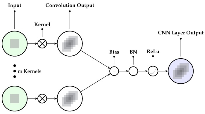
Here, is a rectified linear unit (ReLu) activation function, denotes the batch normalization per activation as further detailed in [50]—it normalizes the convolution output by mean and variance—and represents the bias.
Note, a model with several convolutional layers in a stacked configuration (where the output of layer l is the input for layer ) may be able to learn a hierarchical representation of the data, where deeper layers represent the inputs in a more and more abstract way [18].
Compared to [18], besides a slightly larger kernel size (cf. Table A1 for all hyper parameters), the main difference of the proposed CNN layers is the inclusion of the normalization (BN) to push the activations closer to zero mean and unit variance. In our tests, this gave better results compared to the original convolution layers used in [18]. An explanation for this might be the differences in the data characteristics when mixing simulated and real IMU data for training. Note, network configuration tests are further detailed in Section 4.1. Figure 3 illustrates the convolution from the input to the second layer.
Figure 3.
The CNN layer configuration used in the proposed networks. Note, the Bias, batch normalization (BN) and rectified linear unit (ReLu) operations are applied per activation (see Equation (3)).
2.2.3. Recurrent Neural Network (RNN) Layer
The (feed forward) CNN layers presented in Section 2.2.2 are well suited for learning locally robust features in a time sequence. To represent and learn temporal dynamics of arbitrarily long sequences, a so called RNN has shown to be efficient both regarding its representation power and the required amount of parameters and input data [19,25]. Recurrent neural networks consist of cells with recurrent connections, i.e., forming a directed circle. A drawback of this approach is the problem of vanishing and exploding gradients for long-term dependencies [51]. While there are different approaches to prevent this, we use LSTM and GRU layers, as proposed by [25,52]. In our evaluation the LSTM approach showed the most beneficial behavior for the considered regression problem, while the GRU approach performed best for the classification problem, with comparably less parameters. Note, in [18], only LSTMs were used. Both approaches are further detailed and formalized in Appendix A.
2.2.4. Dropout Layer
To regularize the proposed model, we tested different dropout (statistical regularization) techniques [53]. It was shown that dropout is, on the one hand, more computational efficient than training multiple models for model averaging. On the other hand, it was shown to perform very well in combination with other regularizations, such as -Regularization and Early Stopping [54]. Thus, we evaluated the impact of -Regularization and Early Stopping as regularization methods in addition to dropout, on the same dataset as used for the other configurations, described in Section 4.1. Regarding dropout we tested input dropout with a keep probability of 0.8 [54], naive dropout between the fully connected layers and variational dropout between the RNN layers (latter both with keep probability of 0.5) [55], by taking the same dropout mask in each time step on the input, output and recurrent connections. We achieved the best results with an input dropout of and no dropout between RNN cells as well as between the fully connected layers, in combination with an Regularization with a small weight (see Table A1 in Appendix A).
2.2.5. Application of the Proposed Networks
Applying the above described network configurations to the considered problems has the following implications. For the I2S assignment problem, the output layer is a linear activation with seven hidden nodes that enter the softmax layer resulting in seven probabilities. Here, the highest probability is chosen to represent the predicted IMU location on the lower body (i.e., the I2S assignment). As objective function, we used a cross entropy loss function, during training. Solving the I2S alignment problem requires a suitable rotation parametrization. In order to circumvent the inclusion of additional constraints, we compared two minimal parameterizations in a plausibility test: axis angle and stereographic projection of a unit quaternion [56]. While the former representation is more widespread, it has a singularity around the identity rotation, which can lead to numerical instabilities, if it is not specifically handled. Moreover, the derivatives include irrational sine and cosine terms that are nonlinear and need some sort of approximation during optimization, which can deteriorate convergence and accuracy [56]. The stereographic projection of a quaternion provides a minimal parameterization, for which the derivatives are rational and more. Moreover, there is no singularity for the identity rotation. This parametrization also gave significantly better results in our plausibility tests, which convinced us to use this representation for all further tests. Since the stereographic projection of a unit quaternion is a 3D vector, the output layer mentioned in Section 2.2 is a linear activation with three hidden nodes, the output of which is the predicted I2S alignment. As objective function, we used an loss function, during training.
2.3. Coordinate frames and transformations
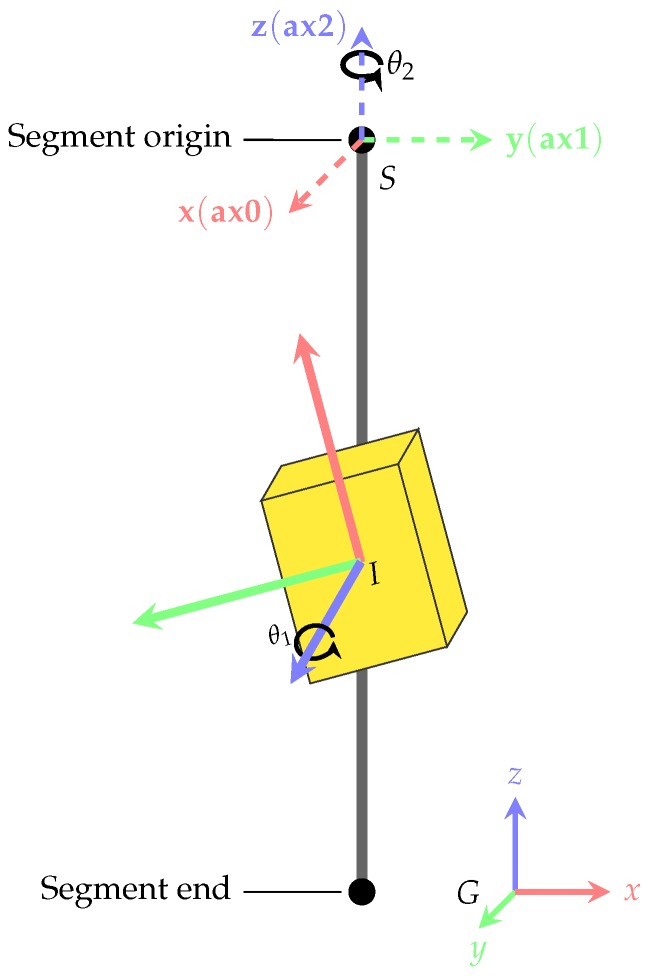
We use three different coordinate frames: The global frame G is a fixed reference frame, S refers to the coordinate frame attached to the considered skeleton segment, and I refers to the coordinate frame attached to the considered IMU (cf. Figure 4). Moreover, the quantities and denote the poses (orientations and positions) of the considered segment and IMU coordinate frames w.r.t. the global frame. From these, the respective I2S orientation (alignment) and position can be obtained as
| (4) |
| (5) |
In addition, given 3D kinematics data in terms of global segment poses () and I2S poses (), the IMU poses can be obtained as
| (6) |
| (7) |
These relations are required for IMU data simulation as detailed in the following Section 2.4. Moreover, denotes the I2S alignment for a given IMU that we want to predict.
Figure 4.
Exemplary illustration of IMU (I), segment (S, dashed) and global (G) coordinate frames for one IMU and one segment. The I2S alignment variations in terms of axes and angles (, ) as basis for IMU data simulation are also illustrated.
2.4. Creation of Artificial Training Data
A major part of this work concerns the mixing of simulated and real IMU training data for increasing the accuracy of the proposed networks w.r.t. the I2S assignment and alignment tasks without the need to record large amounts of training data with alignment variations. This section details the creation of artificial training data in terms of simulated IMU data from available 3D kinematics data (global segment orientations and positions). Here, lower body kinematics data for walking was obtained through own recordings with a commercial IMU based system [57] as well as from an available motion capture dataset [49] (see Section 3.1 for further details on the used datasets). For both sources, the kinematics data were mapped to the skeleton shown in Figure 1. For creating artificial training data, the first step consisted of simulating a suitable set of I2S alignments for each body segment (Section 2.4.1). Note, in this work, we considered variations of the I2S orientations (), while keeping the I2S positions () stationary on the midpoints of the respective segment axes (i.e., inside the bones). The second step consisted of using these I2S alignments together with the global segment poses available from the 3D kinematics data to obtain sets of IMU trajectories for each segment, from which ideally simulated IMU data was obtained through differentiation. This was followed by mimicking different measurement artifacts to obtain realistic IMU data. The latter steps are detailed in Section 2.4.2.
2.4.1. Simulation of I2S Alignment Variations
An illustration of the I2S alignment variation simulation for one segment is shown in Figure 4. The basic idea is to, in a structured way, generate orientation variation samples for each IMU and associated segment according to the assumptions that body segments can be approximated by capsule like surfaces and IMUs are aligned tangentially to these surfaces, i.e., that their z-axes are approximately aligned with the outward pointing surface normals [11]. This can be achieved by systematically sampling rotation angle tuples with being a set of equidistant angle samples (of the full circle) and applying these to both the z-axis of the considered IMU (in the IMU coordinate frame) and the axis that connects segment origin and end, represented in the respective segment coordinate system. Formalizing this results in alignment variations with
| (8) |
Here, is the assumed initial I2S alignment, e.g., an actual alignment used during an IMU based recording and obtained from an N-pose calibration [10]. The symbol denotes a rotation of angle around rotation axis and N depends on the angle step size. For the experiments, we used leading to alignment variations. Note, while always corresponds to the IMU’s z-axis (represented in the IMU coordinate frame), depends on the body location and is chosen as (i.e., the segment’s z-axis represented in the segment coordinate system) for left and right upper and lower legs, for the pelvis and for the feet. The latter approximates the vector between the foot’s origin and the head of the second metatarsal bone projected onto the ground [8]. These choices correspond to the assumed skeleton definition (segment coordinate systems), as further detailed in Section 3.1.
2.4.2. Simulation of Realistic IMU Data
Given a time sequence of global segment poses (i.e., 3D kinematics data) and a set of constant I2S poses as obtained from the procedure described in the previous section (i.e., neglecting soft tissue artifacts), time sequences of IMU poses were calculated using Equation (6). From this, ideal IMU datasets were simulated using standard data differentiation [58]. Note, in order to compensate for measurement artifacts in the used motion capture data, the global segment pose data was preprocessed with a zero lag Butterworth filter of order 8 and a cutoff frequency of 10 Hz [59]. Moreover, quantization artifacts (sensor ranges and digital resolution) were mimicked according to the specifications of the actual IMUs used in this work [57].
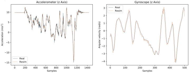
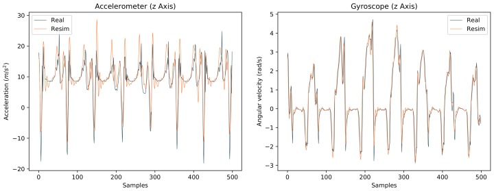
Figure 5 illustrates an example of good correspondence between real and re-simulated IMU data for a plausibility test, where IMUs were rigidly mounted on a rigid body (i.e., excluding soft tissue artifacts) moved freely in space and were additionally tracked with a gold standard marker based optical system [60]. The Pearson correlation coefficients between real and re-simulated accelerometer and gyroscope data were on average for all channels and IMUs and , respectively (see Table A2 and Table A3 in Appendix B).
Figure 5.
Comparison between real and re-simulated IMU data for one example from a capturing setup where IMUs were rigidly mounted on a rigid body and were additionally tracked with a marker based optical system. The frequency was 60 Hz, i.e., 60 samples correspond to one second.
We also compared our results to the simulated IMU data obtained from IMUSim [42] with comparable results (Pearson correlation coefficients when using [42]: and , respectively).
Figure 6 shows an example comparison of real and re-simulated data from a walking motion (IMU on the right foot). Here, the average Pearson correlation coefficients over all channels and all IMUs were for the accelerometers and for the gyroscopes (see Table A4 and Table A5 in Appendix B). The comparably lower correlation coefficient for the accelerometers is shown in Figure 6. Here, the greatest differences between real and re-simulated data are observed during the ground impacts.
Figure 6.
Comparison between real and re-simulated IMU data from the right foot from a capturing setup where IMUs were mounted on a person during walking and were additionally tracked with a marker based optical system. The frequency was 60 Hz, i.e., 60 samples correspond to one second.
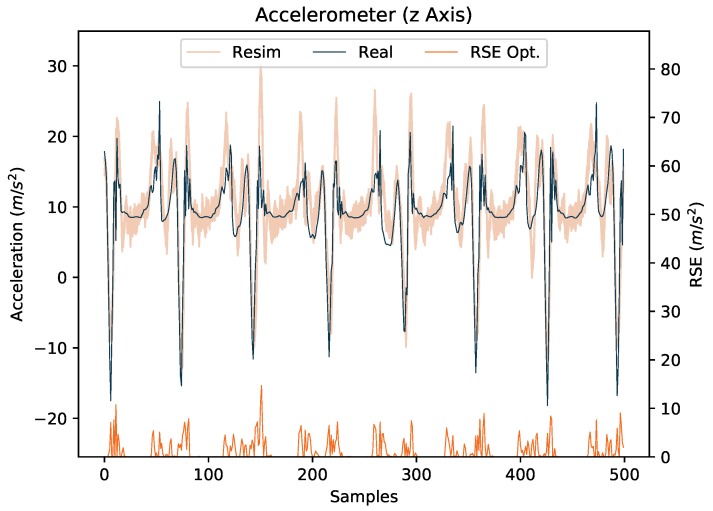
This synthetic gap can be a result of additional artifacts due to clothing or soft-tissue (causing additional accelerations), which are most severe during ground impacts. The approximated I2S position assumption can also add artifacts. To initially address this, inspired by [61], we added zero-mean Gaussian noise (, with = 1 m/s) to all accelerometer channels. Note, we considered the gyroscope data to be reasonable without additional noise, in this work. Figure 7 augments Figure 6 by showing 100 re-simulated noisy signals per timestep. In addition, the absolute errors between real and re-simulated signals are shown.
Figure 7.
Figure 6 augmented with 100 noisy re-simulated signals per timestep and the respective root squared errors (RSE) between the real signal and the closest re-simulated signal at each timestep (RSE Opt.).
Qualitatively speaking, it can be seen in the figure that the real accelerometer signal is often included in the fan of noisy re-simulated signals. Quantitatively, this shows in a drop of the average RMSE over all channels and all IMUs from m/s for a signal without noise to m/s when considering the closest noise sample at each timestep (i.e., the optimal case). Anticipating the experimental results in Section 4, the addition of Gaussian noise resulted in a considerable improvement w.r.t. the addressed I2S assignment and alignment tasks (8 percent and degrees, respectively, for purely training networks on (noisy) simulated IMU data and testing on unseen labeled real IMU data). Hence, we kept this setting for the subsequent experiments and left more sophisticated soft tissue models (e.g., [61]), general motion artifact compensation (e.g., [62]) or specific compensation of walking artifacts to future work.
3. Datasets and Experiments
This section introduces the datasets used to train and evaluate the proposed networks (Section 3.1), the training configuration and time (Section 3.2) as well as the error metrics used for evaluation (Section 3.3).
3.1. Datasets
Three datasets (A,B, and C) were used for training and evaluation. Dataset A extracts walking motions from the publicly available CMU dataset [49]. The latter provides 3D kinematics data captured with a marker based optical motion capture system. The other datasets consist of IMU and 3D kinematics data recorded with the Xsens Awinda MVN Studio software and the Xsens Awinda IMU hardware [57]. More details are given in the following:
-
A
IMU data simulated from the 3D kinematics data of parts of the CMU dataset (42 participants performing different walking styles, see Table A6 in Appendix C). Note, this dataset is distinguished by a high amount of simulated IMU configuration variations (as described in Section 2.4) based on an already high amount of variability in the 3D kinematics data (in terms of persons and walking styles) used for simulation.
-
B
Collected real IMU data from four male participants (mean age: 32, mean weight: 82 kg, mean height: 181 cm) instructed to walk for one minute back and forth (within an area of five by five meters), with nine different IMU configurations as detailed in Appendix C (Table A7).
-
C
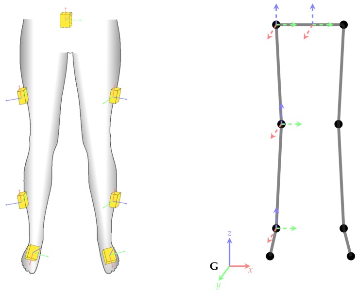
Collected real IMU data from 28 participants (13/15 male/female, mean age: 25 years, mean weight: 70 kg, mean height: 176 cm) instructed to walk for six minutes in an eight-shape within an area of about five by five meters, with one standard IMU configuration, different from the previously mentioned nine configurations (see Figure 8). This study was approved by the Ethical Committee of the University of Kaiserslautern and written informed consent was obtained from all participants prior to their participation.
Figure 8.
(Left) IMU configurations used for the recording of dataset C (dashed lines mark IMUs placed on the back); and (Right) skeleton with exemplary segment coordinate systems of pelvis and right leg (analogous for left leg). The global coordinate system (G) is a fixed reference coordinate system.
3.2. Training
In this work, we utilized methods from the Tensorflow library [63] for training and evaluation of the proposed network configurations. The training was performed on Nvidia GPUs with an average training time of twelve hours for the I2S assignment model and 48 hours for the I2S alignment model. Further details regarding the choice of the optimizer and different hyper parameters can be found in Appendix D (Table A1).
3.3. Evaluation
For model evaluation disjoint training, validation and test sets were created from the above mentioned datasets. According to the leave-one-subject-out (LOSO) method, the test sets consisted of persons not used for training. The training and validation sets were created with a 95% to 5% splitting. The training data were used to train the model. Evaluation on the same data allows verifying whether the model is able to reconstruct the labels of the training data. The validation data were used to evaluate the model on unseen data during the training process. Finally, the test data were used to evaluate the model on data from a person that was not present during the training process. Together, this provides indications of the model’s ability to generalize to unseen data and users.
Two different sets of error measures were used for evaluating the classification and the regression approach. The performance of the classification model was assessed via three scalar measurements based on the classification output in comparison to the ground truth dataset labels, i.e.,
| (9) |
| (10) |
and
| (11) |
The performance of the regression model was assessed by comparing the predicted I2S alignment orientation quaternions () with the ground truth quaternions () for each window i. The orientation deviations () were decomposed into (absolute) angular deviations (, , ) around the x-, y-, z-coordinate axes of the respective segment coordinate frame using an Euler angle decomposition of order (cf. Figure 4). From these measures (which are in the range ) we calculated typical statistics including minimum, maximum, mean, median, and mean squared angular errors in the considered dataset. Note, we also use box plots to illustrate the errors. Here, a white circle denotes the mean, a line across the box denotes the median, a colored bounding box denotes the upper () and lower () quantiles, and whiskers of times the inter quantile range denote the upper and lower bounds.
4. Results and Discussion
This section details the results of applying the proposed methods to the different datasets while moving from simulated to real IMU data. Note, the hyper parameters summarized in Appendix A (Table A1) were obtained through cross validations on dataset A and were used for all experiments. Section 4.1 first provides an evaluation of different network configurations on dataset A, i.e., simulated IMU data for training and evaluation. Section 4.2 then provides evaluation results for the models trained with the proposed (best performing) network configurations (as illustrated in Figure 2) on dataset A. These are subsequently denoted pre-trained models. Thereafter, Section 4.3 evaluates the effects of combining the pre-trained models with simulated and real IMU data for training when testing on real IMU data. This uses dataset B. Finally, Section 4.4 provides an evaluation of the final models using all datasets.
4.1. Evaluation of Network Configurations on Dataset A
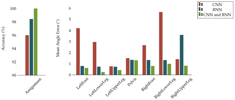
The network configurations described in Section 2.2 (and motivated by [18]) combine CNN and RNN layers. This aims for a model that allows to extract local IMU signal patterns via the CNN layers as well as long-term dependencies via the RNN layers. To evaluate the performances of different network configurations in our considered problems, we performed cross validations using only CNN layers, only RNN layers and a combination of both based on dataset A. The results for both the I2S assignment and alignment tasks are provided in Figure 9 and in Appendix D (Table A8 and Table A9). They clearly confirm the superiority of the proposed combination also for our problems.
Figure 9.
Network configuration cross validation on dataset A: (Left) The bar plot represents the accuracy of the I2S assignment problem; and (Right) the bar plots represent the mean angle errors over all axes and windows for the I2S alignment problem for each body segment.
4.2. Pre-trained Models Based on Dataset A
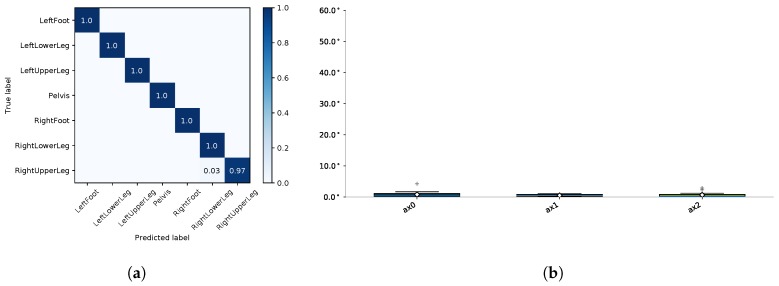
The next step consisted of model training and evaluation on dataset A, i.e., training and testing on simulated IMU data. Figure 10a shows the results for the I2S assignment problem in terms of a confusion matrix. The model achieved 99.99% precision, recall and f-score. Figure 10b shows the results for the I2S alignment problem in terms of box plots of the absolute angular deviations (angle errors) around the three body segment coordinate axes exemplary for the left foot. The mean error over all windows and axes was ° and the maximum error was ° (cf. Figure 9 (right) for average results concerning the other segments).
Figure 10.
Evaluation results on simulated dataset A: (a) confusion matrix for the I2S assignment problem; and (b) boxplots of the angle errors around the three body segment axes for the I2S alignment problem (exemplary for the left foot).
These results attest a good performance of the trained models under controlled conditions (simulated IMU data). Note that we already included Gaussian noise to cover additional real-world effects (cf. Section 2.4.1).
The models trained on dataset A correspond to a proposal distribution generator for an approximate inference from a synthetic data generative model [46], which created the motion samples of dataset A. In the following, these models are denoted pre-trained models.
4.3. Impact of Mixing Real and Simulated IMU Training Data Based on Dataset B
To investigate the effects of combining simulated and real IMU data for training when testing on real IMU data from a person not seen during training, we performed four tests based on dataset B:
Training on real IMU data from three persons (nine alignment variations each, see Table A7 in Appendix C), testing on real IMU data from the left out (test) person (nine alignment variations).
Training on re-simulated IMU data from three persons (64 simulated alignment variations per real IMU alignment), testing on real IMU data from the test person (nine alignment variations).
Setup 2, but with additionally using the real IMU data captured from the three participants (nine alignment variations) for training (i.e., of the training data is based on real IMU data).
Setup 3, with the training being warm-started with the pre-trained models of Section 4.2.
Here, test case 1 can be considered as baseline (training and testing on only few real IMU data), while cases 2 through 4 represent different strategies of using simulated IMU data for increasing the I2S alignment variations present in the training dataset.
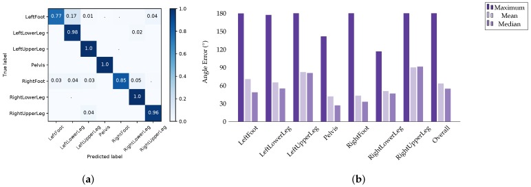
Figure 11a shows the results of test case 1 for the I2S assignment problem. The average accuracy was 94% with the main source of inaccuracy being the feet. Figure 11b shows the results for the I2S alignment problem in terms of per segment mean, median and maximum angle errors over all windows, axes and considered IMU configurations. Here, the model performed rather poorly, with an overall (over all segments) mean angle error of °, average median angle error of ° and maximum angle error of °. This indicates that the training data did not contain sufficient alignment variations for the proposed regression approach.
Figure 11.
Evaluation results on dataset B, test case 1: (a) confusion matrix for the I2S assignment problem; and (b) angle errors over all windows, axes and considered (nine) IMU configurations for the I2S alignment problem for test case 1.
The following sections describe the effects of augmenting the real IMU training data with simulated training data when testing on real IMU data from an unseen person (test cases 2 through 4), first for the I2S assignment then for the I2S alignment problem.
4.3.1. I2S Assignment Problem
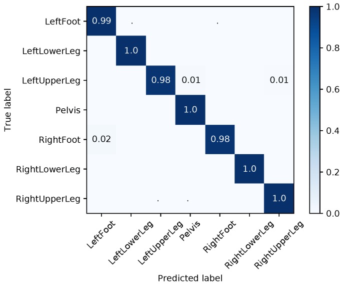
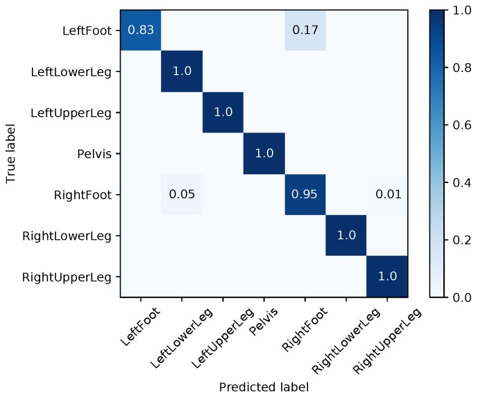
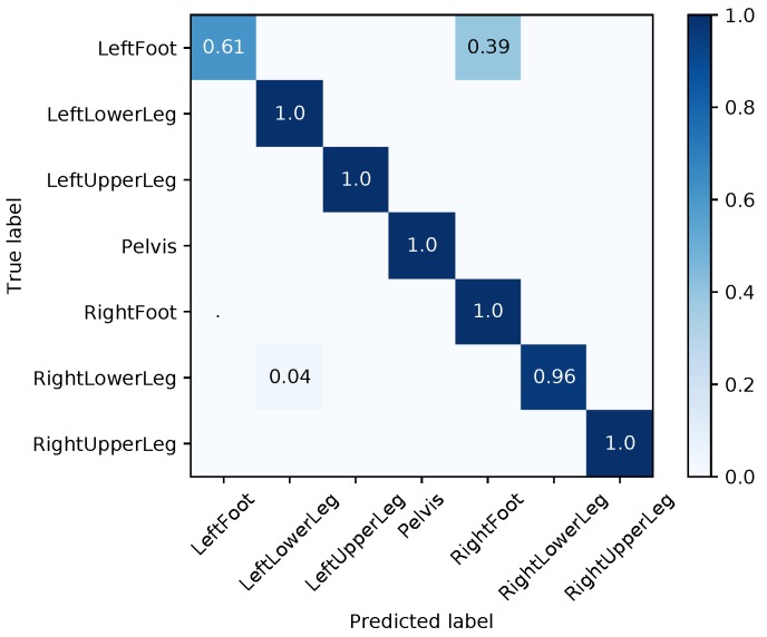
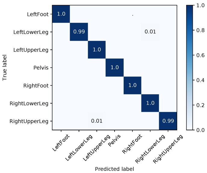
Training on purely simulated data from few participants and then testing on real IMU data from an unseen participant (test case 2) gave an overall accuracy of 68% for the I2S assignment problem. This is a significant decrease compared to the baseline test case 1. Note, the majority of mis-classifications are due to left/right switches that are not explicitly handled in this approach (see Figure 12a). Hence, the prior distribution induced via the few simulated IMU data seems to be insufficient for a high classification accuracy. Adding a small amount of real IMU data to the training set (test case 3) resulted in a performance increase to an average accuracy of (see Figure 12b). Note, the accuracy is still slightly lower compared to the baseline test case 1 (real training data only). Using the pre-trained model from Section 4.2 (based on dataset A) resulted in an average accuracy of (see Figure 12c). This last model performed best with an additional accuracy improvement of as compared to test case 3 (without pre-training) and an increase of compared to the baseline test case 1.
Figure 12.
Evaluation results in terms of confusion matrices for the I2S assignment problem on dataset B.
In summary, these results indicate that a pre-training with simulated IMU data from an existing motion capture dataset (dataset A) in combination with a mixture of simulated and real IMU training data from a small additionally captured dataset (dataset B) yield already promising results for the I2S assignment problem in a real data scenario.
4.3.2. I2S Alignment Problem
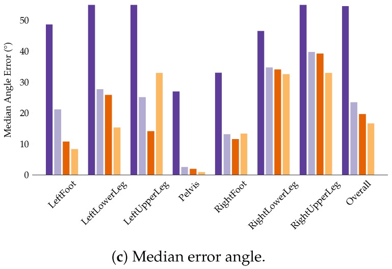
Figure 13 summarizes the evaluation results for test cases 1 through 4 for the I2S alignment problem. Training on purely simulated IMU data (test case 2) resulted in an overall (over all segments) mean angle error over all windows and axes of °. The maximum was ° and the average median was °. This already constitutes a considerable improvement as compared to the baseline test case 1. Adding real IMU data to the training set (test case 3) resulted in a further reduction of the angle errors. The overall mean angle error reduced to °, the maximum to ° and the average median to °. Finally, a slight additional improvement was achieved by using the pre-trained model from Section 4.2 (test case 4). Here, the overall mean, maximum and average median angle error further reduced to °, ° and °, respectively. In summary, these results indicate that our proposed approaches of simulating IMU data and combining the result with real IMU data for training can considerably increase the I2S alignment estimation accuracy when using only a small specifically captured dataset (dataset B).
Figure 13.
Evaluation results for the I2S alignment problem on dataset B. The bar plots show the maximum, mean and median angle errors for all segments over all windows, axes and considered (nine) IMU configurations. These were obtained through cross validation.
4.4. Evaluation of the Final Models
In a last step, final models were trained across all datasets. More specifically, test case 4 in Section 4.3 was extended with real and simulated IMU training data based on dataset C. The final models were tested with two test persons, one randomly selected from dataset B and one randomly selected from dataset C, both not used for training. Hence, the test data included ten different IMU configurations. The following sections describe the evaluation results, first for the I2S assignment then for the I2S alignment problem.
4.4.1. I2S Assignment Problem
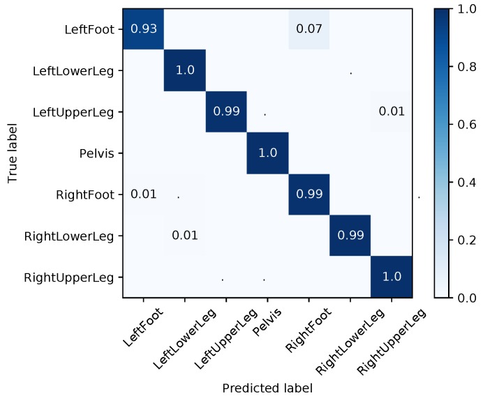
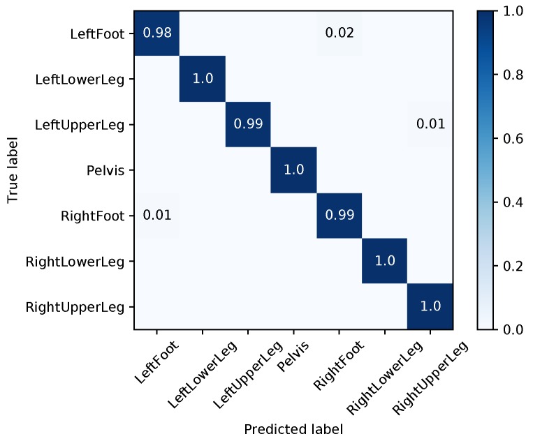
Figure 14 shows the evaluation results (over all test persons/IMU configurations) for the I2S assignment problem. The average accuracy was . We also performed separate evaluations for each different sensor configuration in the test data. The results in terms of confusion matrices are all given in Appendix E (Figure A2, Figure A3, Figure A4, Figure A5, Figure A6, Figure A7, Figure A8, Figure A9, Figure A10 and Figure A11). The average accuracies over all IMUs ranged between and . These results attest a consistently high accuracy for the I2S assignment for a variety of IMU assignments and alignments with our proposed approach. Note that errors only occurred due to left/right leg switches, which are hard to distinguish or even indistinguishable for some cases (if the segments are treated individually as done in our approach).
Figure 14.
Evaluation results in terms of a confusion matrix for the I2S assignment problem using the final model (based on all datasets).
4.4.2. I2S Alignment Problem
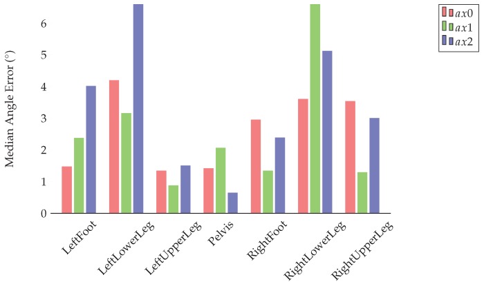
Figure 15 summarizes the evaluation results for the I2S alignment problem in terms of the average median angle errors for all axes over all windows, test persons and IMU configurations. With an overall (over all windows, axes, segments, test persons and IMU configurations) mean angle error of ° and average median of °, the results further improved considerably compared to test case 4 in Section 4.3.2 (the maximum was slightly higher with °) (see Table A10 in Appendix E for additional results). Hence, the addition of a higher amount of real IMU data (with one IMU configuration) completed with simulated alignment variations further increased the degree of generalization of the trained networks.
Figure 15.
Evaluation results for the I2S alignment problem using the final model (based on all datasets). The bar plots show the median angle errors around the three body segment axes over all windows, considered test persons and IMU configurations.
5. Conclusions
The aim of this work was to investigate the potential of deep learning for the challenging tasks of I2S assignment and alignment w.r.t. a biomechanical lower body model based on windows of IMU data (angular velocities, accelerations). We used only small data windows (128 samples) in order to obtain a real-time capable approach. Moreover, we considered each IMU separately in order to obtain an easily adaptable approach for applications in both inertial body motion capture (which is often based on multiple IMUs) and human activity recognition (which often uses a single IMU). Moreover, we aimed at using only a limited amount of real IMU data (in terms of I2S alignments) for training in order to obtain a practical approach.
We confronted these challenges by combining real IMU data samples with additional artificially generated IMU data based on available and newly captured 3D kinematics data. The generation of artificial IMU data was based on the simulation of I2S alignment variations followed by the simulation of noisy IMU data, where the noise was added to reduce the synthetic gap. For both the I2S assignment and alignment determination we utilized a suitable combination of CNN and RNN (LSTM and GRU) based neural network approach.
Regarding the evaluation results on real IMU data, the most promising approach consisted of combining simulated and real IMU data for training, while warm-starting the training with models pre-trained on a purely simulated dataset.
For the I2S assignment problem we achieved average accuracy on a small newly recorded dataset with only four persons and nine I2S alignment variations. This was improved to by augmenting the real training data with simulated I2S alignment variations and by starting from a pre-trained model based on purely simulated IMU data (see Section 4.3). With a further increase of the amount of real IMU data (eight-shaped walking from 28 persons and one standard I2S alignment) we obtained an average accuracy of (see Section 4.4). Note, the remaining errors were only due to left/right switches. The segments (pelvis, upper leg, lower leg, and foot) where identified with accuracy. Hence, a reliable left/right assignment is one part of our future work.
For the I2S alignment problem we achieved significant improvements when mixing real and simulated IMU data for training. When training and testing on the newly captured dataset with only four persons and nine I2S alignment variations the angle errors were rather large, e.g., ° overall mean angle error, ° overall maximum angle error and ° overall median angle error (Section 4.3). This, however, considerably improved to an overall mean of °, maximum of ° and median of ° when augmenting the real training data with simulated I2S alignment variations and by starting from the pre-trained model (see Section 4.3). When increasing the amount of real IMU data for training as mentioned above the proposed approach showed an additional improvement (overall mean and median angle errors of ° and °, respectively). The observed outliers (overall maximum of °) were likely caused by real-world effects that were not yet sufficiently covered by the training dataset (e.g., amount of real I2S alignment variations and movement variations, soft tissue artifacts, and I2S position offsets).
Altogether, these results demonstrate the feasibility of augmenting real IMU training data with simulated data for improving the recognition/estimation accuracies. Note that the proposed approach provides I2S assignment and alignment of, in principle, any number of IMUs (they are treated separately) to the lower body skeleton in about two seconds of walking (assuming 60 Hz frequency) without using magnetometer data.
To further improve the validity and reliability of the proposed approach, there are a few interesting avenues for future research: the inclusion of uncertainties into the proposed approach, e.g., based on Bayesian deep learning [53] to provide indications for reliable I2S alignment estimates; a reliable left/right assignment; and an extension to the full body. In general, a more sophisticated approach for IMU data simulation, e.g., based on more realistic body shapes [64], a better soft tissue model, possibly such as the one used in [61], and the modeling of I2S position offsets could further reduce the synthetic gap in IMU data simulation and by this the amount of outliers and the required amount of real data.
Acknowledgments
This work was performed by the Interdisciplinary Junior Research Group wearHEALTH at the University of Kaiserslautern, funded by the BMBF (16SV7115), in cooperation with the Augmented Vision Department at DFKI Kaiserslautern. We thank Didier Stricker for supporting this work. For more information, please visit the websites www.wearhealth.org and av.dfki.de.
Appendix A. Proposed Network Configurations
Appendix A.1. Long Short-Term Memory (LSTM)
The core of the LSTM networks are the LSTM cells that replace the recurrent connections in the RNN approach with gated cells. The idea is that the recurrence is jointly trained with gates, which in turn control the information flow through the cell and are therefore able to counteract the vanishing and exploding gradient problem. LSTMs have been shown to learn long time dependencies more easily than RNNs. Note that these dependencies can also reach over a considered input window of data. The input to the LSTM cell consists of an activation at time t () and the output of the previous hidden state of the cell . The hidden state is usually initialized with . The LSTM cell consists of different components. The cell state is updated in a controlled manner, via different gates. The forget gate controls the amount of information from past cell states that should be prevented from influencing future cell states. It is updated as
| (A1) |
Here and in the following, the subscripts of the matrices denote the from-to relationship [18], i.e., is a matrix that relates the (input) activation vector to the vector f(t) representing the forget gate. relates the hidden state and f(t). The activation function is a tangens-hyperbolicus (tanh) function and denotes a bias. The input gate controls the amount of information that is allowed to modify the cell state via the hidden state and current activation. It is updated as
| (A2) |
As above, and are matrices, is a bias vector and a tanh function. The cell state is updated with a conditional self-loop, weighted by the forget gate vector and the update weighted by the input gate vector
| (A3) |
Here, ⊙ denotes an element-wise multiplication. Again, and denote matrices, denotes a bias vector and is a tanh function. Finally, the output gate vector and the hidden state at the next timestep () are computed as
| (A4) |
| (A5) |
Again, and are matrices, is a bias vector and are tanh functions.
Appendix A.2. Gated Recurrent Unit (GRU)
In contrast to an LSTM cell, the GRU cell, as introduced in [52], fuses forget and input gate to an update gate. Further, it merges the cell and hidden states. This results in a reduced amount of parameters and, hence, a simpler model. Similar to the LSTM cell, a new state is computed as a linear sum between the previous and current determined state, although GRU cells do not provide a mechanism for controlling the degree of state exposure. The state, , is computed as
| (A6) |
where denotes the candidate state and the update gate. The update gate, which determines the degree to which the previous cell state and the candidate state contribute to the cell update, is updated as
| (A7) |
where and are weight matrices, as in Appendix A.1. The candidate state is related to the calculation of a traditional recurrent unit as in [65]. It is updated as
| (A8) |
Here, represents the reset gate, and are matrices, is a tanh function and denotes the activation. Similar to the update gate , the reset gate is computed as
| (A9) |
where , are matrices and is a tanh function. This finishes the update of the GRU cell.
Appendix A.3. Hyper Parameters
Table A1.
Hyper parameters of the proposed network configurations, determined through cross validation based on dataset A and used for all tests.
| Assignment | Alignment | ||
|---|---|---|---|
| Optimizer | Batch size | 256 | 256 |
| Learning rate | 0.001 | 0.001 | |
| Optimizer | Adam | Adam | |
| CNN Layer | # Layer | 3 | 3 |
| Kernel | 16 × 1 | 16 × 1 | |
| # Kernel | 64 | 64 | |
| RNN Layer | # Layer | 1 | 2 |
| Cell | GRU | LSTM | |
| # Units | 128 | 128 | |
| Regularization | -Factor | 0.0001 | 0.0001 |
| Keep probability | 0.8 | 0.8 |
Appendix B. IMU Data Simulation
Table A2.
Pearson correlation coefficients and root mean squared errors (RMSE) between real and re-simulated accelerometer data from a capturing setup where the seven IMUs used in the experiments were rigidly mounted on a rigid body and were additionally tracked with a marker based optical system.
| Accelerometer (Pearson Correlation Coefficient) | ||||
| IMU | mean | |||
| 1 | 0.9903 | 0.9915 | 0.9862 | 0.9893 |
| 2 | 0.9901 | 0.9898 | 0.9819 | 0.9873 |
| 3 | 0.9913 | 0.9909 | 0.9854 | 0.9892 |
| 4 | 0.9918 | 0.9828 | 0.9762 | 0.9836 |
| 5 | 0.9917 | 0.9875 | 0.9819 | 0.9870 |
| 6 | 0.9897 | 0.9869 | 0.9756 | 0.9841 |
| 7 | 0.9908 | 0.9920 | 0.9866 | 0.9898 |
| mean | 0.9908 | 0.9888 | 0.9820 | 0.9872 |
| Accelerometer RMSE [m/s] | ||||
| mean | ||||
| 1 | 0.6950 | 0.6969 | 0.7934 | 0.7285 |
| 2 | 0.7190 | 0.7977 | 0.9613 | 0.8260 |
| 3 | 0.6506 | 0.6991 | 0.7894 | 0.7130 |
| 4 | 0.6814 | 0.9577 | 1.0750 | 0.9047 |
| 5 | 0.6640 | 0.8111 | 0.9024 | 0.7925 |
| 6 | 0.7534 | 0.9265 | 1.2443 | 0.9747 |
| 7 | 0.6869 | 0.6644 | 0.7574 | 0.7029 |
| mean | 0.6929 | 0.7933 | 0.9319 | 0.8060 |
Table A3.
Pearson correlation coefficients and root mean squared errors (RMSE) between real and re-simulated gyroscope data from a capturing setup where the seven IMUs used in the experiments were rigidly mounted on a rigid body and were additionally tracked with a marker based optical system.
| Gyroscope (Pearson Correlation Coefficient) | ||||
| IMU | mean | |||
| 1 | 0.9594 | 0.9760 | 0.9778 | 0.9711 |
| 2 | 0.9637 | 0.9793 | 0.9737 | 0.9722 |
| 3 | 0.9645 | 0.9800 | 0.9759 | 0.9734 |
| 4 | 0.9617 | 0.9798 | 0.9753 | 0.9723 |
| 5 | 0.9640 | 0.9798 | 0.9750 | 0.9729 |
| 6 | 0.9632 | 0.9816 | 0.9776 | 0.9742 |
| 7 | 0.9652 | 0.9800 | 0.9766 | 0.9739 |
| mean | 0.9631 | 0.9795 | 0.9760 | 0.9729 |
| Gyroscope RMSE [rad/s] | ||||
| IMU | mean | |||
| 1 | 0.5978 | 0.3519 | 0.2661 | 0.4053 |
| 2 | 0.5671 | 0.3252 | 0.2904 | 0.3942 |
| 3 | 0.5604 | 0.3210 | 0.2782 | 0.3865 |
| 4 | 0.5840 | 0.3236 | 0.2811 | 0.3962 |
| 5 | 0.5636 | 0.3231 | 0.2834 | 0.3901 |
| 6 | 0.5838 | 0.3060 | 0.2700 | 0.3866 |
| 7 | 0.5558 | 0.3193 | 0.2745 | 0.3832 |
| mean | 0.5732 | 0.3243 | 0.2777 | 0.3917 |
Table A4.
Pearson correlation coefficients and root mean squared errors (RMSE) between real and re-simulated accelerometer data from a capturing setup where IMUs were mounted on a person during walking and were additionally tracked with a marker based optical system.
| Accelerometer (Pearson Correlation Coefficient) | ||||
| IMU | mean | |||
| LeftLowerLeg | 0.7428 | 0.4830 | 0.6028 | 0.6095 |
| RightUpperLeg | 0.5726 | 0.2803 | 0.7139 | 0.5223 |
| LeftUpperLeg | 0.6717 | 0.1602 | 0.7737 | 0.5352 |
| RightLowerLeg | 0.7325 | 0.3326 | 0.5148 | 0.5266 |
| LeftFoot | 0.8067 | 0.3962 | 0.6565 | 0.6198 |
| Pelvis | 0.8132 | 0.2409 | 0.4940 | 0.5161 |
| RightFoot | 0.8456 | 0.4342 | 0.8026 | 0.6942 |
| mean | 0.7407 | 0.3325 | 0.6512 | 0.5748 |
| Accelerometer RMSE [m/s] | ||||
| IMU | mean | |||
| LeftLowerLeg | 3.6462 | 4.3371 | 4.1111 | 4.0314 |
| RightUpperLeg | 4.2053 | 3.2582 | 3.8274 | 3.7637 |
| LeftUpperLeg | 3.1212 | 3.9498 | 3.4068 | 3.4926 |
| RightLowerLeg | 3.9041 | 5.0482 | 4.3344 | 4.4289 |
| LeftFoot | 5.3138 | 4.9329 | 4.7109 | 4.9859 |
| Pelvis | 2.2677 | 2.5007 | 2.3478 | 2.3720 |
| RightFoot | 4.6748 | 6.4197 | 4.0363 | 5.0436 |
| mean | 3.8762 | 4.3495 | 3.8250 | 4.0169 |
Table A5.
Pearson correlation coefficients and root mean squared errors (RMSE) between real and re-simulated gyroscope data from a capturing setup where IMUs were mounted on a person during walking and were additionally tracked with a marker based optical system.
| Gyroscope (Pearson Correlation Coefficient) | ||||
| IMU | mean | |||
| LeftLowerLeg | 0.8720 | 0.9802 | 0.9628 | 0.9383 |
| RightUpperLeg | 0.8736 | 0.9570 | 0.9207 | 0.9171 |
| LeftUpperLeg | 0.8661 | 0.9692 | 0.8901 | 0.9085 |
| RightLowerLeg | 0.8681 | 0.9820 | 0.9469 | 0.9323 |
| LeftFoot | 0.9145 | 0.9618 | 0.9234 | 0.9332 |
| Pelvis | 0.9778 | 0.8890 | 0.9349 | 0.9339 |
| RightFoot | 0.8451 | 0.9673 | 0.9504 | 0.9209 |
| mean | 0.8882 | 0.9581 | 0.9327 | 0.9263 |
| Gyroscope RMSE [rad/s] | ||||
| IMU | mean | |||
| LeftLowerLeg | 0.8678 | 0.5459 | 0.2285 | 0.5474 |
| RightUpperLeg | 0.6663 | 0.4652 | 0.1804 | 0.4373 |
| LeftUpperLeg | 0.8404 | 0.3579 | 0.2251 | 0.4745 |
| RightLowerLeg | 0.7338 | 0.5556 | 0.1653 | 0.4849 |
| LeftFoot | 0.6386 | 1.0709 | 0.4129 | 0.7075 |
| Pelvis | 0.1287 | 0.1257 | 0.0938 | 0.1161 |
| RightFoot | 0.4638 | 1.0177 | 0.4836 | 0.6550 |
| mean | 0.6199 | 0.5913 | 0.2557 | 0.4890 |
Appendix C. Datasets
Table A6.
List of the 42 participants and recordings used from the CMU dataset [49] to create dataset A.
| Participant ID | Recording | Frames | Duration [s] | Motion Description |
|---|---|---|---|---|
| 02 | 01 | 313 | 313. | Walk |
| 02 | 298 | 298. | Walk | |
| 03 | 01 | 432 | 432. | Walk on uneven terrain |
| 02 | 365 | 365. | Walk on uneven terrain | |
| 03 | 4563 | 4563. | Walk on uneven terrain | |
| 04 | 4722 | 4722. | Walk on uneven terrain | |
| 05 | 01 | 598 | 598. | Walk |
| 06 | 01 | 494 | 494. | Walk |
| 07 | 01 | 316 | 316. | Walk |
| 02 | 329 | 329. | Walk | |
| 03 | 415 | 415. | Walk | |
| 04 | 449 | 449. | Slow walk | |
| 05 | 517 | 517. | Slow walk | |
| 06 | 417 | 417. | Walk | |
| 07 | 379 | 379. | Walk | |
| 08 | 362 | 362. | Walk | |
| 09 | 306 | 306. | Walk | |
| 10 | 301 | 301. | Walk | |
| 11 | 315 | 315. | Walk | |
| 08 | 01 | 277 | 277. | Walk |
| 02 | 309 | 309. | Walk | |
| 03 | 353 | 353. | Walk | |
| 04 | 484 | 484. | Slow walk | |
| 06 | 296 | 296. | Walk | |
| 08 | 283 | 283. | Walk | |
| 09 | 293 | 293. | Walk | |
| 10 | 275 | 275. | Walk | |
| 10 | 04 | 549 | 549. | Walk |
| 12 | 01 | 523 | 523. | Walk |
| 02 | 673 | 673. | Walk | |
| 03 | 565 | 565. | Walk | |
| 15 | 01 | 5524 | 5524. | Walk / wander |
| 03 | 12550 | 12550. | Walk/wander | |
| 09 | 7875 | 7875. | Walk/wander | |
| 14 | 9003 | 9003. | Walk/wander | |
| 16 | 15 | 471 | 471. | Walk |
| 16 | 510 | 510. | Walk | |
| 21 | 312 | 312. | Walk | |
| 22 | 307 | 307. | Walk | |
| 31 | 424 | 424. | Walk | |
| 32 | 580 | 580. | Walk | |
| 47 | 416 | 416. | Walk | |
| 58 | 342 | 342. | Walk | |
| 26 | 01 | 833 | 833. | Walk |
| 27 | 01 | 1033 | 1033. | Walk |
| 29 | 01 | 1316 | 1316. | Walk |
| 32 | 01 | 482 | 482. | Walk |
| 02 | 434 | 434. | Walk | |
| 36 | 01 | 557 | 557. | Walk on uneven terrain |
| 04 | 3726 | 3726. | Walk on uneven terrain | |
| 05 | 4196 | 4196. | Walk on uneven terrain | |
| 06 | 3896 | 3896. | Walk on uneven terrain | |
| 07 | 3772 | 3772. | Walk on uneven terrain | |
| 08 | 3714 | 3714. | Walk on uneven terrain | |
| 10 | 3832 | 3832. | Walk on uneven terrain | |
| 11 | 4168 | 4168. | Walk on uneven terrain | |
| 12 | 4585 | 4585. | Walk on uneven terrain | |
| 13 | 4247 | 4247. | Walk on uneven terrain | |
| 14 | 4146 | 4146. | Walk on uneven terrain | |
| 15 | 4164 | 4164. | Walk on uneven terrain | |
| 16 | 4395 | 4395. | Walk on uneven terrain | |
| 17 | 4359 | 4359. | Walk on uneven terrain | |
| 18 | 4304 | 4304. | Walk on uneven terrain | |
| 19 | 4193 | 4193. | Walk on uneven terrain | |
| 20 | 4090 | 4090. | Walk on uneven terrain | |
| 21 | 4030 | 4030. | Walk on uneven terrain | |
| 22 | 4312 | 4312. | Walk on uneven terrain | |
| 23 | 4392 | 4392. | Walk on uneven terrain | |
| 24 | 4153 | 4153. | Walk on uneven terrain | |
| 25 | 4685 | 4685. | Walk on uneven terrain | |
| 26 | 4237 | 4237. | Walk on uneven terrain | |
| 27 | 4247 | 4247. | Walk on uneven terrain | |
| 28 | 2391 | 2391. | Walk on uneven terrain | |
| 29 | 4469 | 4469. | Walk on uneven terrain | |
| 30 | 4414 | 4414. | Walk on uneven terrain | |
| 31 | 3736 | 3736. | Walk on uneven terrain | |
| 32 | 4468 | 4468. | Walk on uneven terrain | |
| 33 | 4311 | 4311. | Walk on uneven terrain | |
| 34 | 4328 | 4328. | Walk on uneven terrain | |
| 35 | 4341 | 4341. | Walk on uneven terrain | |
| 36 | 4792 | 4792. | Walk on uneven terrain | |
| 37 | 01 | 511 | 511. | Slow walk |
| 38 | 01 | 352 | 352. | Walk |
| 02 | 420 | 420. | Walk | |
| 39 | 01 | 378 | 378. | Walk |
| 02 | 400 | 400. | Walk | |
| 03 | 407 | 407. | Walk | |
| 04 | 410 | 410. | Walk | |
| 05 | 400 | 400. | Walk | |
| 06 | 368 | 368. | Walk | |
| 07 | 367 | 367. | Walk | |
| 08 | 350 | 350. | Walk | |
| 10 | 395 | 395. | Walk | |
| 11 | 391 | 391. | Walk | |
| 12 | 427 | 427. | Walk | |
| 13 | 378 | 378. | Walk | |
| 14 | 399 | 399. | Walk | |
| 43 | 01 | 421 | 421. | Walk |
| 45 | 01 | 456 | 456. | Walk |
| 46 | 01 | 616 | 616. | Walk |
| 49 | 01 | 652 | 652. | Walk |
| 55 | 01 | 530 | 530. | Walk |
| 69 | 01 | 469 | 469. | Walk forward |
| 02 | 343 | 343. | Walk forward | |
| 03 | 430 | 430. | Walk forward | |
| 04 | 426 | 426. | Walk forward | |
| 05 | 453 | 453. | Walk forward | |
| 81 | 02 | 544 | 544. | Walk forward |
| 03 | 1076 | 1076. | Walk | |
| 17 | 916 | 916. | Walk forward | |
| 91 | 04 | 2162 | 2162. | Walk |
| 10 | 3175 | 3175. | Slow walk | |
| 17 | 1520 | 1520. | Quick walk | |
| 22 | 2106 | 2106. | Casual quick walk | |
| 27 | 2894 | 2894. | Slow walk | |
| 29 | 2181 | 2181. | Walk | |
| 31 | 1992 | 1992. | Walk | |
| 34 | 2208 | 2208. | Walk | |
| 57 | 1177 | 1177. | Walk forward | |
| 93 | 07 | 236 | 236. | Casual walk |
| 103 | 07 | 236 | 236. | Casual walk |
| 104 | 19 | 921 | 921. | Casual walk |
| 35 | 1074 | 1074. | Slow walk | |
| 356 | 2315 | 2315. | Slow walk | |
| 105 | 03 | 1865 | 1865. | Walk |
| 10 | 3175 | 3175. | Slow walk | |
| 17 | 1520 | 1520. | Quick walk | |
| 22 | 2106 | 2106. | Casual quick walk | |
| 27 | 2894 | 2894. | Slow walk | |
| 29 | 2181 | 2181. | Walk | |
| 57 | 1177 | 1177. | Walk forward | |
| 111 | 34 | 1837 | 1837. | Walk |
| 35 | 1503 | 1503. | Walk | |
| 113 | 25 | 689 | 689. | Walk |
| 114 | 13 | 3132 | 3132. | Walk |
| 14 | 5854 | 5854. | Walk | |
| 15 | 1384 | 1384. | Walk | |
| 120 | 19 | 12792 | 12792. | Slow walk |
| 20 | 10735 | 10735. | Walk | |
| 132 | 17 | 268 | 268. | Walk fast |
| 18 | 425 | 425. | Walk fast | |
| 19 | 271 | 271. | Walk fast | |
| 20 | 342 | 342. | Walk fast | |
| 21 | 354 | 354. | Walk fast | |
| 22 | 371 | 371. | Walk fast | |
| 45 | 1531 | 1531. | Walk slow | |
| 46 | 1223 | 1223. | Walk slow | |
| 47 | 1510 | 1510. | Walk slow | |
| 48 | 1625 | 1625. | Walk slow | |
| 49 | 1748 | 1748. | Walk slow | |
| 50 | 2139 | 2139. | Walk slow | |
| 133 | 21 | 786 | 786. | Walk |
| 22 | 759 | 759. | Walk | |
| 23 | 848 | 848. | Walk | |
| 136 | 24 | 1075 | 1075. | Walk |
| 137 | 29 | 1128 | 1128. | Walk |
| 139 | 28 | 2970 | 2970. | Walk |
| 30 | 1261 | 1261. | Walk | |
| 141 | 19 | 1193 | 1193. | Walk |
| 25 | 614 | 614. | Walk | |
| 143 | 32 | 780 | 780. | Walk |
| 144 | 33 | 4688 | 4688. | Walk |
Table A7.
IMU configurations used during the recording of dataset B.
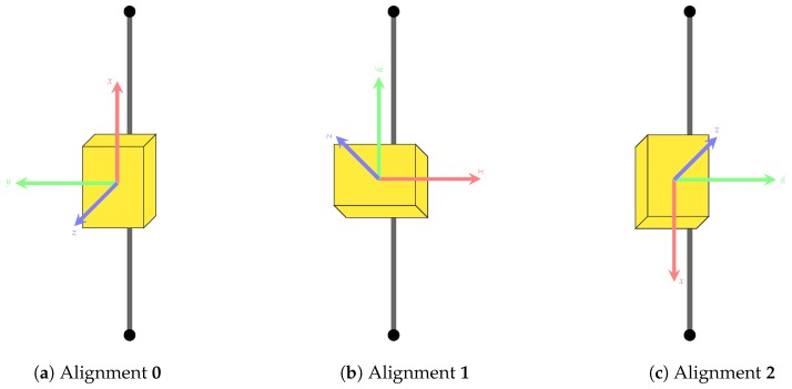
| Placement on Segment | Alignment (See Figure A1) | ||||
|---|---|---|---|---|---|
| # | Upper Leg | Lower Leg | Foot | Pelvis | |
| 1 | anterior | anterior | dorsal | posterior | 0 |
| 2 | anterior | anterior | dorsal | posterior | 1 |
| 3 | anterior | anterior | dorsal | posterior | 2 |
| 4 | lateral | lateral | dorsal | posterior | 0 |
| 5 | lateral | lateral | dorsal | posterior | 1 |
| 6 | lateral | lateral | dorsal | posterior | 2 |
| 7 | anterior | medial | dorsal | posterior | 0 |
| 8 | anterior | medial | dorsal | posterior | 1 |
| 9 | anterior | medial | dorsal | posterior | 2 |
Figure A1.
IMU alignments used during the recording of dataset B.
Appendix D. Cross Validation Results on Dataset A
Table A8.
Results of the architecture cross validation for the I2S assignment problem based on dataset A.
| Accuracy in % | |||
|---|---|---|---|
| CNN | RNN | CNN and RNN | |
| Assignment | 96.00 | 98.43 | 100.00 |
Table A9.
Results of the architecture cross validation for the I2S alignment problem based on dataset A: mean angle errors over all axes and windows for each segment.
| Mean Angle Errors | |||
|---|---|---|---|
| CNN | RNN | CNN and RNN | |
| LeftFoot | 4.201 | 0.796 | 0.623 |
| LeftLowerLeg | 2.955 | 0.736 | 0.252 |
| LeftUpperLeg | 0.770 | 0.729 | 0.427 |
| Pelvis | 1.503 | 1.347 | 1.309 |
| RightFoot | 2.670 | 1.336 | 0.800 |
| RightLowerLeg | 5.649 | 1.329 | 0.990 |
| RightUpperLeg | 1.407 | 3.589 | 0.822 |
| Mean | 2.736 | 1.405 | 0.795 |
Appendix E. Evaluation Results for the Final Models
Figure A2, Figure A3, Figure A4, Figure A5, Figure A6, Figure A7, Figure A8, Figure A9, Figure A10 and Figure A11 show the evaluation results in terms of confusion matrices for the I2S assignment problem based on the final model. Each confusion matrix corresponds to one (of ten) combination(s) of test person (dataset B or C) and IMU configuration (cf. Table A7 and Figure 8). Table A10 shows the evaluation results for the I2S alignment problem.
Figure A2.
I2S assignment problem, final model: test person from dataset B, IMU configuration 1 (cf. Table A7). Average accuracy: .
Figure A3.
I2S assignment problem, final model: test person from dataset B, IMU configuration 2 (cf. Table A7). Average accuracy: .
Figure A4.
I2S assignment problem, final model: test person from dataset B, IMU configuration 3 (cf. Table A7). Average accuracy: .
Figure A5.
I2S assignment problem, final model: test person from dataset B, IMU configuration 4 (cf. Table A7). Average accuracy: .
Figure A6.
I2S assignment problem, final model: test person from dataset B, IMU configuration 5 (cf. Table A7). Average accuracy: .
Figure A7.
I2S assignment problem, final model: test person from dataset B, IMU configuration 6 (cf. Table A7). Average accuracy: .
Figure A8.
I2S assignment problem, final model: test person from dataset B, IMU configuration 7 (cf. Table A7). Average accuracy: .
Figure A9.
I2S assignment problem, final model: test person from dataset B, IMU configuration 8 (cf. Table A7). Average accuracy: .
Figure A10.
I2S assignment problem, final model: test person from dataset B, IMU configuration 9 (cf. Table A7). Average accuracy: .
Figure A11.
I2S assignment problem, final model: test person from dataset C, IMU configuration according to Figure 8). Average accuracy: .
Table A10.
I2S alignment problem, final model, all test persons and IMU configurations: median, mean and maximum angle errors around the three body segment axes.
| Segment | |||||||||
|---|---|---|---|---|---|---|---|---|---|
| Med | Mean | Max | Med | Mean | Max | Med | Mean | Max | |
| LeftFoot | 1.48 | 13.71 | 165.06 | 2.38 | 6.99 | 44.70 | 4.02 | 12.21 | 155.23 |
| LeftLowerLeg | 4.20 | 28.59 | 178.40 | 3.16 | 14.22 | 75.82 | 7.04 | 17.95 | 116.93 |
| LeftUpperLeg | 1.35 | 14.35 | 171.09 | 0.88 | 8.40 | 81.11 | 1.51 | 10.13 | 96.67 |
| Pelvis | 1.42 | 13.53 | 180.00 | 2.07 | 7.28 | 88.45 | 0.65 | 12.89 | 179.98 |
| RightFoot | 2.96 | 16.12 | 127.48 | 1.35 | 5.23 | 72.81 | 2.39 | 11.42 | 157.63 |
| RightLowerLeg | 3.61 | 31.21 | 179.97 | 7.63 | 10.92 | 52.61 | 5.13 | 24.49 | 179.79 |
| RightUpperLeg | 3.54 | 28.55 | 178.10 | 1.30 | 9.42 | 77.72 | 3.02 | 21.79 | 179.64 |
| Average | 2.65 | 20.86 | 168.58 | 2.68 | 8.92 | 70.46 | 3.39 | 15.84 | 152.26 |
Author Contributions
T.Z. designed and implemented the system, contributed to the design of the experiments and conducted the experiments, analyzed the data and contributed to writing the article. B.T. supervised the design and implementation of the system, designed the experiments and supervised their conduction, analyzed the results and wrote the article. G.B. contributed to data analysis and writing of the article.
Conflicts of Interest
The authors declare no conflict of interest.
References
- 1.Fong D.T.P., Chan Y.Y. The use of wearable inertial motion sensors in human lower limb biomechanics studies: A systematic review. Sensors. 2010;10:11556–11565. doi: 10.3390/s101211556. [DOI] [PMC free article] [PubMed] [Google Scholar]
- 2.Patel S., Park H., Bonato P., Chan L., Rodgers M. A review of wearable sensors and systems with application in rehabilitation. J. NeuroEng. Rehabil. 2012;9:21. doi: 10.1186/1743-0003-9-21. [DOI] [PMC free article] [PubMed] [Google Scholar]
- 3.Hadjidj A., Souil M., Bouabdallah A., Challal Y., Owen H. Wireless sensor networks for rehabilitation applications: Challenges and opportunities. J. Netw. Comput. Appl. 2013;36:1–15. doi: 10.1016/j.jnca.2012.10.002. [DOI] [Google Scholar]
- 4.Zheng Y.L., Ding X.R., Poon C.C.Y., Lo B.P.L., Zhang H., Zhou X.L., Yang G.Z., Zhao N., Zhang Y.T. Unobtrusive sensing and wearable devices for health informatics. IEEE Trans. Biomed. Eng. 2014;61:1538–1554. doi: 10.1109/TBME.2014.2309951. [DOI] [PMC free article] [PubMed] [Google Scholar]
- 5.Bleser G., Taetz B., Miezal M., Christmann C.A., Steffen D., Regenspurger K. Development of an Inertial Motion Capture System for Clinical Application—Potentials and challenges from the technology and application perspectives. J. Interact. Media. 2017;16 doi: 10.1515/icom-2017-0010. [DOI] [Google Scholar]
- 6.Roetenberg D., Luinge H., Slycke P. Xsens MVN: Full 6DOF Human Motion Tracking Using Miniature Inertial Sensors. Xsens Technologies; Enschede, The Netherlands: 2014. Technical report. [Google Scholar]
- 7.Miezal M., Taetz B., Bleser G. On Inertial Body Tracking in the Presence of Model Calibration Errors. Sensors. 2016;16:1132. doi: 10.3390/s16071132. [DOI] [PMC free article] [PubMed] [Google Scholar]
- 8.Miezal M., Taetz B., Bleser G. Real-time inertial lower body kinematics and ground contact estimation at anatomical foot points for agile human locomotion; Proceedings of the International Conference on Robotics and Automation; Singapore. 29 May–3 June 2017. [Google Scholar]
- 9.Bouvier B., Duprey S., Claudon L., Dumas R., Savescu A. Upper Limb Kinematics Using Inertial and Magnetic Sensors: Comparison of Sensor-to-Segment Calibrations. Sensors. 2015;15:18813–18833. doi: 10.3390/s150818813. [DOI] [PMC free article] [PubMed] [Google Scholar]
- 10.Palermo E., Rossi S., Marini F., Patané F., Cappa P. Experimental evaluation of accuracy and repeatability of a novel body-to-sensor calibration procedure for inertial sensor-based gait analysis. Measurement. 2014;52:145–155. doi: 10.1016/j.measurement.2014.03.004. [DOI] [Google Scholar]
- 11.Taetz B., Bleser G., Miezal M. Towards self-calibrating inertial body motion capture; Proceedings of the International Conference on Information Fusion; Heidelberg, Germany. 5–8 July 2016; pp. 1751–1759. [Google Scholar]
- 12.Weenk D., Van Beijnum B.J.F., Baten C.T., Hermens H.J., Veltink P.H. Automatic identification of inertial sensor placement on human body segments during walking. J. NeuroEng. Rehabil. 2013;10:1. doi: 10.1186/1743-0003-10-31. [DOI] [PMC free article] [PubMed] [Google Scholar]
- 13.Graurock D., Schauer T., Seel T. Automatic pairing of inertial sensors to lower limb segments—A plug-and-play approach. Curr. Direct. Biomed. Eng. 2016;2:715–718. doi: 10.1515/cdbme-2016-0155. [DOI] [Google Scholar]
- 14.De Vries W., Veeger H., Cutti A., Baten C., van der Helm F. Functionally interpretable local coordinate systems for the upper extremity using inertial & magnetic measurement systems. J. Biomech. 2010;43:1983–1988. doi: 10.1016/j.jbiomech.2010.03.007. [DOI] [PubMed] [Google Scholar]
- 15.Favre J., Aissaoui R., Jolles B., de Guise J., Aminian K. Functional calibration procedure for 3D knee joint angle description using inertial sensors. J. Biomech. 2009;42:2330–2335. doi: 10.1016/j.jbiomech.2009.06.025. [DOI] [PubMed] [Google Scholar]
- 16.Attal F., Mohammed S., Dedabrishvili M., Chamroukhi F., Oukhellou L., Amirat Y. Physical Human Activity Recognition Using Wearable Sensors. Sensors. 2015;15:31314–31338. doi: 10.3390/s151229858. [DOI] [PMC free article] [PubMed] [Google Scholar]
- 17.Davis K., Owusu E., Bastani V., Marcenaro L., Hu J., Regazzoni C., Feijs L. Activity recognition based on inertial sensors for Ambient Assisted Living; Proceedings of the 19th International Conference on Information Fusion (FUSION); Heidelberg, Germany. 5–8 July 2016; pp. 371–378. [Google Scholar]
- 18.Ordóñez F.J., Roggen D. Deep Convolutional and LSTM Recurrent Neural Networks for Multimodal Wearable Activity Recognition. Sensors. 2016;16:115. doi: 10.3390/s16010115. [DOI] [PMC free article] [PubMed] [Google Scholar]
- 19.Goodfellow I., Bengio Y., Courville A. Deep Learning. MIT Press; Cambridge, UK: 2016. [(accessed on 14 January 2018)]. Available online: http://www.deeplearningbook.org. [Google Scholar]
- 20.Ciresan D.C., Meier U., Masci J., Schmidhuber J. Multi-column deep neural network for traffic sign classification. Neural Netw. 2012;32:333–338. doi: 10.1016/j.neunet.2012.02.023. [DOI] [PubMed] [Google Scholar]
- 21.Krizhevsky A., Sutskever I., Hinton G.E. ImageNet Classification with Deep Convolutional Neural Networks. In: Pereira F., Burges C.J.C., Bottou L., Weinberger K.Q., editors. Advances in Neural Information Processing Systems 25. Curran Associates, Inc.; New York, NY, USA: 2012. pp. 1097–1105. [Google Scholar]
- 22.Ji S., Xu W., Yang M., Yu K. 3D Convolutional Neural Networks for Human Action Recognition. IEEE Trans. Pattern Anal. Mach. Intell. 2013;35:221–231. doi: 10.1109/TPAMI.2012.59. [DOI] [PubMed] [Google Scholar]
- 23.Tewari A., Taetz B., Grandidier F., Stricker D. Advances in Visual Computing, Proceedings of the 12th International Symposium, ISVC 2016, Las Vegas, NV, USA, 12–14 December 2016. Springer International Publishing; Basel, Switzerland: 2016. Two Phase Classification for Early Hand Gesture Recognition in 3D Top View Data; pp. 353–363. [Google Scholar]
- 24.Tewari A., Taetz B., Frederic G., Stricker D. A Probablistic Combination of CNN and RNN Estimates for Hand Gesture Based Interaction in Car; Proceedings of the IEEE International Symposium on Mixed and Augmented Reality (ISMAR); Nantes, France. 9–13 October 2017. [Google Scholar]
- 25.Hochreiter S., Schmidhuber J. Long short-term memory. Neural Comput. 1997;9:1735–1780. doi: 10.1162/neco.1997.9.8.1735. [DOI] [PubMed] [Google Scholar]
- 26.Schmidhuber J. Deep learning in neural networks: An overview. Neural Netw. 2015;61:85–117. doi: 10.1016/j.neunet.2014.09.003. [DOI] [PubMed] [Google Scholar]
- 27.Alsheikh M.A., Selim A., Niyato D., Doyle L., Lin S., Tan H.P. Cornell University Library; 2016. [(accessed on 14 January 2018)]. Deep Activity Recognition Models with Triaxial Accelerometers. Technical Report. Available online: https://arxiv.org/abs/1511.04664. [Google Scholar]
- 28.Morales F.J.O.N., Roggen D. Deep Convolutional Feature Transfer Across Mobile Activity Recognition Domains, Sensor Modalities and Locations; Proceedings of the 2016 ACM International Symposium on Wearable Computers; Heidelberg, Germany. 12–16 September 2016; New York, NY, USA: ACM; 2016. pp. 92–99. [Google Scholar]
- 29.Kunze K., Lukowicz P. Sensor placement variations in wearable activity recognition. IEEE Pervasive Comput. 2014;13:32–41. doi: 10.1109/MPRV.2014.73. [DOI] [Google Scholar]
- 30.Pannurat N., Thiemjarus S., Nantajeewarawat E., Anantavrasilp I. Analysis of Optimal Sensor Positions for Activity Classification and Application on a Different Data Collection Scenario. Sensors. 2017;17:774. doi: 10.3390/s17040774. [DOI] [PMC free article] [PubMed] [Google Scholar]
- 31.Kunze K., Lukowicz P. Dealing with Sensor Displacement in Motion-based Onbody Activity Recognition Systems; Proceedings of the 10th International Conference on Ubiquitous Computing; Seoul, Korea. 21–24 September 2008; New York, NY, USA: ACM; 2008. pp. 20–29. [Google Scholar]
- 32.Jiang M., Shang H., Wang Z., Li H., Wang Y. A method to deal with installation errors of wearable accelerometers for human activity recognition. Physiol. Meas. 2011;32:347. doi: 10.1088/0967-3334/32/3/006. [DOI] [PubMed] [Google Scholar]
- 33.Henpraserttae A., Thiemjarus S., Marukatat S. Accurate Activity Recognition Using a Mobile Phone Regardless of Device Orientation and Location; Proceedings of the International Conference on Body Sensor Networks, BSN 2011; Dallas, TX, USA. 23–25 May 2011; pp. 41–46. [Google Scholar]
- 34.Kunze K., Lukowicz P., Junker H., Tröster G. Where am i: Recognizing on-body positions of wearable sensors; Proceedings of the International Symposium on Location- and Context-Awareness; Oberpfaffenhofen, Germany. 12–13 May 2005; Basel, Switzerland: Springer International Publishing; 2005. pp. 264–275. [Google Scholar]
- 35.Amini N., Sarrafzadeh M., Vahdatpour A., Xu W. Accelerometer-based on-body sensor localization for health and medical monitoring applications. Pervasive Mob. Comput. 2011;7:746–760. doi: 10.1016/j.pmcj.2011.09.002. [DOI] [PMC free article] [PubMed] [Google Scholar]
- 36.Mannini A., Sabatini A.M., Intille S.S. Accelerometry-based recognition of the placement sites of a wearable sensor. Pervasive Mob. Comput. 2015;21:62–74. doi: 10.1016/j.pmcj.2015.06.003. [DOI] [PMC free article] [PubMed] [Google Scholar]
- 37.Fujinami K., Jin C., Kouchi S. Tracking on-body location of a mobile phone; Proceedings of the International Symposium on Wearable Computers; Seoul, Korea. 10–13 October 2010; pp. 190–197. [Google Scholar]
- 38.Kunze K., Lukowicz P. Using acceleration signatures from everyday activities for on-body device location; Proceedings of the 2007 11th IEEE International Symposium on Wearable Computers; Boston, MA, USA. 11–13 October 2007; 2007; pp. 115–116. [Google Scholar]
- 39.Xu W., Zhang M., Sawchuk A.A., Sarrafzadeh M. Robust human activity and sensor location corecognition via sparse signal representation. IEEE Trans. Biomed. Eng. 2012;59:3169–3176. doi: 10.1109/TBME.2012.2211355. [DOI] [PubMed] [Google Scholar]
- 40.Shi Y., Shi Y., Liu J. A Rotation Based Method for Detecting On-body Positions of Mobile Devices. Proceedings of the 13th International Conference on Ubiquitous Computing, Beijing, China, 17–21 September 2011. ACM; New York, NY, USA: 2011. pp. 559–560. [Google Scholar]
- 41.Thiemjarus S. A Device-Orientation Independent Method for Activity Recognition; Proceedings of the International Conference on Body Sensor Networks, BSN 2010; Singapore. 7–9 June 2010; pp. 19–23. [Google Scholar]
- 42.Young A.D., Ling M.J., Arvind D.K. IMUSim: A Simulation Environment for Inertial Sensing Algorithm Design and Evaluation; Proceedings of the 10th International Conference on Information Processing in Sensor Networks; Chicago, IL, USA. 12–14 April 2011; pp. 199–210. [Google Scholar]
- 43.Brunner T., Lauffenburger J., Changey S., Basset M. Magnetometer-Augmented IMU Simulator: In-Depth Elaboration. Sensors. 2015;15:5293–5310. doi: 10.3390/s150305293. [DOI] [PMC free article] [PubMed] [Google Scholar]
- 44.Ligorio G., Bergamini E., Pasciuto I., Vannozzi G., Cappozzo A., Sabatini A.M. Assessing the Performance of Sensor Fusion Methods: Application to Magnetic-Inertial-Based Human Body Tracking. Sensors. 2016;16:153. doi: 10.3390/s16020153. [DOI] [PMC free article] [PubMed] [Google Scholar]
- 45.Zhang X., Fu Y., Jiang S., Sigal L., Agam G. Cornell University Library; 2015. [(accessed on 14 January 2018)]. Learning from Synthetic Data Using a Stacked Multichannel Autoencoder. Technical Report. Available online: https://arxiv.org/abs/1509.05463. [Google Scholar]
- 46.Le T.A., Baydin A.G., Zinkov R., Wood F. Using Synthetic Data to Train Neural Networks is Model-Based Reasoning. arXiv. 2017. 1703.00868v1
- 47.Zhang X., Fu Y., Zang A., Sigal L., Agam G. Cornell University Library; 2015. [(accessed on 14 January 2018)]. Learning Classifiers from Synthetic Data Using a Multichannel Autoencoder. Technical Report. Available online: https://arxiv.org/abs/1503.03163. [Google Scholar]
- 48.Simard P.Y., Steinkraus D., Platt J.C. Best Practices for Convolutional Neural Networks Applied to Visual Document Analysis; Proceedings of the Seventh International Conference on Document Analysis and Recognition (ICDAR ’03); Edinburgh, UK. 3–6 August 2003; Washington, DC, USA: IEEE Computer Society; 2003. [Google Scholar]
- 49.University C.M. CMU Graphics Lab Motion Capture Database Website. [(accessed on 14 January 2018)]; Available online: http://mocap.cs.cmu.edu/
- 50.Ioffe S., Szegedy C. Batch normalization: Accelerating deep network training by reducing internal covariate shift; Proceedings of the International Conference on Machine Learning; Lille, France. 6–1 July 2015; pp. 448–456. [Google Scholar]
- 51.Bengio Y., Simard P., Frasconi P. Learning long-term dependencies with gradient descent is difficult. IEEE Trans. Neural Netw. 1994;5:157–166. doi: 10.1109/72.279181. [DOI] [PubMed] [Google Scholar]
- 52.Cho K., van Merrienboer B., Gülcehre C., Bahdanau D., Bougares F., Schwenk H., Bengio Y. In: Learning Phrase Representations using RNN Encoder-Decoder for Statistical Machine Translation. Moschitti A., Pang B., Daelemans W., editors. Association for Computational Linguistics; Doha, Qatar: 2014. pp. 1724–1734. EMNLP. [Google Scholar]
- 53.Gal Y. Ph.D. Thesis. University of Cambridge; Cambridge, UK: 2016. Uncertainty in Deep Learning. [Google Scholar]
- 54.Srivastava N., Hinton G.E., Krizhevsky A., Sutskever I., Salakhutdinov R. Dropout: A simple way to prevent neural networks from overfitting. J. Mach. Learn. Res. 2014;15:1929–1958. [Google Scholar]
- 55.Gal Y. A Theoretically Grounded Application of Dropout in Recurrent Neural Networks. arXiv. 2015. 1512.05287
- 56.Terzakis G., Culverhouse P., Bugmann G., Sharma S., Sutton R. A Recipe on the Parameterization of Rotation Matrices for Non-Linear Optimization Using Quaternions. Marine and Industrial Dynamic Analysis School of Marine Science and Engineering, Plymouth University; Plymouth, UK: 2012. Technical report, Technical report MIDAS. SMSE. 2012. TR. 004; [Google Scholar]
- 57.Xsens Technologies B.V. [(accessed on 14 January 2018)]; Available online: https://www.xsens.com/products/xsens-mvn/
- 58.Shuster M.D. A survey of attitude representations. Navigation. 1993;8:439–517. [Google Scholar]
- 59.Butterworth S. On the theory of filter amplifiers. Wirel. Eng. 1930;7:536–541. [Google Scholar]
- 60.NaturalPoint OptiTrack. [(accessed on 14 January 2018)]; Available online: http://www.optitrack.com/motion-capture-biomechanics/
- 61.Olsson F., Halvorsen K. Experimental evaluation of joint position estimation using inertial sensors; Proceedings of the 20th International Conference on Information Fusion (Fusion), IEEE; Xi’an, China. 10–13 July 2017; pp. 1–8. [Google Scholar]
- 62.Mohammed S., Tashev I. Unsupervised deep representation learning to remove motion artifacts in free-mode body sensor networks; Proceedings of the 14th IEEE International Conference on Wearable and Implantable Body Sensor Networks (BSN); Eindhoven, The Netherlands. 9–12 May 2017; pp. 183–188. [Google Scholar]
- 63.Abadi M., Agarwal A., Barham P., Brevdo E., Chen Z., Citro C., Corrado G.S., Davis A., Dean J., Devin M., et al. Tensorflow: Large-scale machine learning on heterogeneous distributed systems. arXiv. 2016. 1603.04467
- 64.Golyanik V., Reis G., Taetz B., Strieker D. A framework for an accurate point cloud based registration of full 3D human body scans; Proceedings of the 2017 Fifteenth IAPR International Conference on Machine Vision Applications (MVA); Nagoya, Japan. 8–12 May 2017; pp. 67–72. [Google Scholar]
- 65.Bahdanau D., Cho K., Bengio Y. Neural machine translation by jointly learning to align and translate. arXiv. 2014. 1409.0473


