Prediction of Breast Cancer Risk Using a Machine Learning Approach Embedded with a Locality Preserving Projection Algorithm

Abstract

In order to automatically identify a set of effective mammographic image features and build an optimal breast cancer risk stratification model, this study aims to investigate advantages of applying a machine learning approach embedded with a locally preserving projection (LPP) based feature combination and regeneration algorithm to predict short-term breast cancer risk. A dataset involving negative mammograms acquired from 500 women was assembled. This dataset was divided into two age-matched classes of 250 high risk cases in which cancer was detected in the next subsequent mammography screening and 250 low risk cases, which remained negative. First, a computer-aided image processing scheme was applied to segment fibro-glandular tissue depicted on mammograms and initially compute 44 features related to the bilateral asymmetry of mammographic tissue density distribution between left and right breasts. Next, a multi-feature fusion based machine learning classifier was built to predict the risk of cancer detection in the next mammography screening. A leave-one-case-out (LOCO) cross-validation method was applied to train and test the machine learning classifier embedded with a LLP algorithm, which generated a new operational vector with 4 features using a maximal variance approach in each LOCO process. Results showed a 9.7% increase in risk prediction accuracy when using this LPP-embedded machine learning approach. An increased trend of adjusted odds ratios was also detected in which odds ratios increased from 1.0 to 11.2. This study demonstrated that applying LPP algorithm effectively reduced feature dimensionality, and yielded higher and potentially more robust performance in predicting short-term breast cancer risk.

1. INTRODUCTION

In spite of the heterogeneity of breast cancer, mammographic screening is widely considered the most effective approach to detect breast cancer at an early stage and help reduce the cancer mortality rate (Narol et al 2014). Among the existing screening methods, mammography is the only clinically accepted screening modality applied to the general population to date (Saslow et al 2007). Despite significant advantages of mammography screening (i.e., relatively lower cost, wide accessibility and short examination time), controversy about the population-based mammography screening remains (Berlin et al 2010) because of its lower sensitivity among a number of groups of women (i.e., women who are younger than 50 years old and have dense breasts (Carney et al 2003)) and high false-positive recall rates (Hubbard et al 2011). Thus, in order to improve efficacy of mammography screening, establishing a new personalized breast cancer screening paradigm has recently been attracting extensive research interests (Brawley et al 2012). One of the important prerequisites for realizing this goal is to identify and develop effective clinical markers or prediction tools, which have higher discriminatory power to predict the risk or likelihood of individual women having or developing image-detectable cancer in a short-term (i.e., < 2 to 5 years after a negative screening) (Zheng et al 2012).

Although a number of epidemiology-based breast cancer risk prediction models (i.e., Gail (Gail et al 1989) and Tyrer-Cuzick (Tyrer et al 2004) models) have been developed and used to identify high risk women, these models have low positive predictive values to help determine who should be screened in the short-term and who can be screened at longer intervals in order to increase cancer detection yield and reduce unnecessarily frequent screening and the associated false-positive recalls with mammography (Gail et al 2010). Therefore, it requires identifying and developing more effective cancer risk prediction markers including those generated from genomic tests (Van Ziteren et al 2011) and image analysis (Wei et al 2011). In the medical imaging field, breast density assessed from mammograms is considered an imaging marker or risk factor with much higher discriminatory power than the most of other risk factors used in the existing breast cancer risk prediction models (Amir et al 2010). However, subjectively rating mammographic density by radiologists based on the Breast Imaging Reporting and Data System (BIRADS) guideline is often not reliable due to large intra- and inter-reader variability (Berg et al 2000). In order to produce more robust results in assessing mammographic density and identifying new imaging markers to predict breast cancer risk, a number of computer-aided image processing schemes have been developed to segment and compute Volumetric Breast Density (VBD) from mammograms to predict breast cancer risk (e.g., (Damases et al 2016)). However, whether the computed mammographic density can accurately represent breast density remains controversial (Kopans et al 2008). The assessed mammographic density may vary due to the change of the imaging machines, imaging acquisition protocol and life cycle of the women.

In order to avoid or minimize the impact of inconsistency when using mammographic density as a breast cancer risk factor, we recently explored a new breast cancer risk factor or a quantitative imaging marker based on the bilateral asymmetry of mammographic tissue density between the left and right breasts to predict short-term breast cancer risk (Zheng et al 2012, Zheng et al 2014). Since two bilateral mammograms are acquired from the same woman at one mammography screening, the relative mammographic density asymmetry is likely to remain highly consistent. From bilateral mammograms, we are able to compute a large number of image features to represent difference of mammographic tissue density patterns. Thus, how to identify and assemble an optimal set of effective and non-redundant image features from the initial feature pool with a large number of computed image features remains a technical challenge. In order to address this challenge, the objective of this study is to develop and apply a new machine learning approach to create a small effective feature vector for the purpose of building an optimal machine learning classifier using a relatively small training image dataset. Inspired by the deep learning technology, which directly uses input images to generate an efficient feature vector for classification (Shen et al 2017), we proposed to apply a locally preserving projection (LPP) based feature combination algorithm (He et al 2004) to reduce dimensionality of feature space and then build a new image features based short-term breast cancer risk prediction model. Unlike the conventional feature selection methods that filter and select a set of existing optimal features from the initial feature pools, LPP generates a new optimal feature vector involving features that are different from any original features in the existing feature pool. The details of the proposed LLP approach, our image dataset, experiment and data analysis results are presented in the following sections of this article.

2. MATERIALS & METHOD

2.1. Image Dataset

A testing image dataset was retrospectively assembled for this study, which includes two sets of sequential full-field digital mammography (FFDM) images acquired from 500 women participated in mammography screening. In the first set of FFDM screening, all images were determined negative by the radiologists. These negative images are named as “prior” images in this study. In the second set of FFDM screening, 250 cases were positive with cancer detected by the radiologists and verified by biopsy and histopathology tests, while other 250 cases remained negative. All negative cases remained cancer-free for at least two more subsequent FFDM screenings. Images in the second set of screening are named as “current” images. The time interval between the “prior” and “current” mammography screenings ranged from 12 to 18 months. Although all “prior” FFDM screenings were negative, we divided 500 cases into two classes. The first class includes 250 high-risk cases in which cancer was developed and detected in the “current” FFDM screening. The second class includes 250 low-risk cases that remained negative in the “current” FFDM screening.

Table 1 summarizes additional dataset information, which includes distribution of women age and mammographic density rated by radiologists based on BIRADS guidelines. In this dataset, age ranged between 38 and 88 years old. This is also an age-matched image dataset (≤ 1 year difference between the two classes of the cases). Thus, it has no statistically significant difference of ages between the high and low risk case classes (p = 0.12). There is also no significant difference in BIRADS based mammographic density ratings between two classes. In this study, two “prior” negative FFDM images acquired from bilateral cranio-caudal (CC) view of left and right breasts were selected and used.

Table 1.

Distribution of age and density BIRADS of cases in the dataset

		High Risk Class	Low Risk Class
Age	Mean	58.84	57.39
	> 65 years old	57	48
	45–65 years old	174	170
	< 45 years old	19	32
BIRADS	Extremely dense (4)	6	7
	Heterogenous (3)	133	131
	Scattered (2)	100	99
	Fatty tissue (1)	11	13

2.2. A Computer-aided Imaging Processing Scheme

We developed and applied a computer-aided image processing scheme to automatically segment dense fibro-glandular breast tissue regions depicted on each mammogram, and then computed bilateral mammographic tissue density and feature asymmetry between the left and right CC view images. Figure 1 shows a graphic user interface (GUI) of the image processing scheme. After a user selects a testing case by pointing the computer mouse to one image name of the case and clicking the mouse button, a pair of two bilateral CC view images is uploaded into the GUI simultaneously. From each originally digital mammogram, the scheme automatically segments breast region and generates several image maps.

Figure 1.

Illustration of the graphic user interface of our computer-aided imaging processing scheme to detect bilateral mammographic image feature asymmetry and predict short-term breast cancer risk.

First, a fibro-glandular tissue (FGT) density map is generated from each original mammogram as shown in Figure 2(a). The percentage of FGT on each mammogram can be quantitative computed. In addition, since mammograms are two-dimensional projection images, each pixel value (or gray level) represents a percentage of the fibro-glandular tissues along the projection line (or path) of the X-ray. In order to increase the visual sensitivity to the tissue density variation, a pseudo color coding is applied to the FGT density map displayed in GUI. Second, from the FGT map, the scheme searches and segments focally dense regions as shown in Figure 2(b). Third, the scheme generates a local density fluctuation map as shown in Figure 2(c) using the method reported in our previous studies of developing computer-aided detection (CAD) scheme of mammograms (Zheng et al 2006) and mammographic image feature based cancer risk prediction model (Wang et al 2011). Last, the scheme applies a difference of Gaussian (DOG) bandpass filter to generate a map showing the distribution of locally isolated small dense regions (or blobs). A similar DOG filtering map has been used in the previous CAD scheme of mammograms as the first step to detect suspicious lesions (Zheng et al 1995).

Figure 2.

An example of showing the intermediate results of image processing steps including (a) computed breast tissue density maps, (b) detected focal density regions, (c) local density (pixel value) fluctuation maps, and (d) image maps generated using Gaussian bandpass filtering. Color bars show volumetric density level of the pixel values.

2.3. Image Feature Computation

Since early breast cancer usually develops in one breast, the bilateral asymmetry of mammographic tissue density or feature patterns is typically the first importantly visual sign for radiologists to detect breast abnormalities that have a high risk of leading to the cancer development. Based on the observation of how radiologists read and interpret mammograms, we identified a new quantitative imaging marker to predict short-term breast cancer risk. Our previous study has demonstrated a trend of increasing bilateral asymmetry of the computed bilateral mammographic density features as the time lag between the negative and positive mammography screening reduces (Tan et al 2016).

First, our computer-aided scheme calculated a series of global statistical image features related to the pixel value distribution of each image or map, which include mean, standard deviation, skewness and kurtosis of pixel value distribution in one original digital mammogram (as shown in Figure 1) and 4 sets of computer-processed image maps (as shown in Figure 2). Then, the scheme computed each bilateral asymmetry (or difference) of the image feature value by combining two corresponding feature values computed from the two bilateral images or maps between the left and right breasts. Typically, for each feature, scheme computes and generates three combined features. First, an average feature value, $F_{\mathit{ave}}=\frac{1}{2}\times (F_{\mathit{left}}+F_{\mathit{right}})$, represents a global mammographic density related feature of each testing case. For example, a case with dense breasts has higher average pixel values computed from the original mammograms and FGT maps than a case of fatty breasts. Second, an absolute feature difference value, F_ad = |F_left − F_right|, or difference ratio, F_adr = |F_left − F_right|/(F_left + F_right), indicates bilateral feature asymmetry between left and right breasts. Third, a multiplication value of above 2 features, F_M = F_ave × F_ad, considers the contribution of these two factors. For example, the contribution of the bilateral asymmetry levels to the cancer risk at breasts with different mammographic density may be different. Table 2 lists the 44 computed image features and their definition.

Table 2.

Description of 44 computed image features in the initial feature pool

Image	Feature Number	Feature Description
Original FFDM image	1 – 3	Average and absolute difference of density values, and multiplication of above 2 features.
FGT map	4 – 7	Average and absolute difference of mean high density value, difference ratio and multiplication of the first 2 features.
	8 – 10	Average and absolute difference of FGT volume, and multiplication of above two features.
	11 – 13	Average and absolute difference of standard deviation of pixel values, and multiplication.
	14 – 17	Average and absolute difference of skewness and kurtosis of pixel values.
Focal density map	18 – 21	Average and absolute difference of focal density value, difference ratio and multiplication of the first 2 features.
	22 – 29	Average and absolute difference of mean, standard deviation, skewness, and kurtosis of detected and segmented focal density regions.
Local fluctuation map	29 – 33	Average of mean, standard deviation, skewness and kurtosis of pixel values.
	34 – 37	Absolute difference of mean, standard deviation, skewness and kurtosis of pixel values.
	38 – 41	Multiplication of average and absolute difference of mean, standard deviation, skewness and kurtosis of pixel values
DOG map	42 – 44	Average and absolute difference of mean pixel values, multiplication of above 2 features.

2.4. Machine Learning Generated Imaging Marker

Applying a machine learning method to generate an optimal and robust multi-feature fusion based imaging marker or prediction model depends on two factors namely, (1) a set of effective and non-redundant image features, and (2) a relatively large and diverse dataset. Figure 3 compares 3 types of machine learning methods. First, in the conventional machine learning as shown in Figure 3(a), segmentation and feature extraction steps are indispensable. A specific number of features from the initial feature pool are selected based on a predefined evaluation method and index. Then, the selected features are used to build the classifier. Second, a deep learning technique does not require handcrafted features computed from the well-segmented regions. It automatically identifies features by directly learning and analyzing input images as shown in Figure 3(b). However, in order to achieve robust results, the deep learning method typically requires a very large training dataset, which is often not available in the cancer imaging field.

Figure 3.

Block Diagram of three types of risk model systems, (a) conventional systems for feature selection and classification, (b) deep learning techniques for feature generation and classification, (c) proposed method for feature extraction, regeneration, and classification.

It is clear by comparing between conventional and deep machine learning methods, each has advantages and disadvantages. Conventional machine learning uses handcrafted image features, wherein it is often difficult to identify an optimal set of features that can be most effectively fused together to achieve the best performance. However, conventional machine learning is relatively easy to train using small dataset. Deep learning has the capability to automatically determine more effective features and their combination by directly learning from the input images, but its performance heavily depends on the size and diversity of training dataset.

Figure 3(c) shows a new two-step approach tested in this study, which aims to take advantages of both conventional and deep machine learning approaches. Similar to a conventional learning method, this approach includes a regular region segmentation and feature extraction step to compute image features and build an initial feature pool. Then, the approach applies an LLP algorithm to learn and analyze the initially computed image features and automatically regenerate a new feature vector. This is similar to the deep learning approach, which is possible to extract new features using a deep convolution neural network (CNN) model for direct image feature learning and pass the CNN-generated features to the input layer of a conventional machine learning model, such as a support vector machine (SVM), to perform a specific classification task. However, comparing to the direct image based deep learning technique, the number of inputs (44 features as shown in Table 2 as comparing to large pixel number of an input image) is significantly reduced in this study, so that a conventional machine learning classifier embedded with the LPP image feature regeneration algorithm has potential to be more robustly trained and tested using a relatively small dataset.

Thus, we first used a locally preserving projection (LPP) based feature combination algorithm (He et al 2004) to generated new features. LPP is an unsupervised subspace learning method and a linear approximation of non-linear Laplacian eigenmap. It involves linear projective maps to find a graph of embedding in a specific way to preserve local structure information. It has been tested and demonstrated high performance and advantages in feature dimensionality reduction, information retrieval and pattern classification or recognition. It models the manifold structure directly by constructing the nearest-neighbor graph of neighborhood information of the dataset. This graph reveals neighborhood relations of data samples. By using the Laplacian technique, transformation matrix of the dataset is generated to map the originally big feature space to a much compact and more effective subspace. This linear procedure also preserves local neighborhood information of the input dataset. The procedure of LPP can be summarized as the following three steps (He et al 2004).

1. Construct adjacent graph using ε-neighborhood or k-neighborhood.

   1. ε-neighborhood. The system connects nodes i and j by an edge if |x_i − x_j|² < ε.

   2. k-neighborhood: The system connects nodes i and j by an edge if i is in k NNs of j or j is in k NNs of i.

2. Compute weight matrix W by using either uniform weight or Gaussian weight of Euclidean distance. If nodes i and j are connected, then:

   $$w_{ij}=\{\begin{array}{ll}exp({\Vert a_i-u_9\Vert }^2/t);\hfill & \hfill x_j\in N_k(x_i),or{x}_i\in N_k(x_j)\\ 0\hfill & \hfill \mathit{otherwise}\end{array}$$ (1)

   where parameter t is a positive constant and t ∈ R, and N_k(X_i) or N_k(X_j) denotes a set of the k NNs of the sample x_i or x_j.

3. Construct the final Eigenmap. The transformation matrix P is optimized by computing the minimum eigenvalue solution to the generalized eigenvalue problem as (2):

   $${\mathit{XLX}}^{T}P=\lambda {\mathit{XDX}}^{T}P$$ (2)

   where D is a diagonal matrix. A summation on the column of W makes elements of D, D_ii = ΣW_jj. L = D − W is the Laplacian matrix. In this equation P is composed of the optimal r projection vectors corresponding to the r smallest eigenvalues, i.e. λ₁ ≤ λ₂ ≤ ··· ≤ λ_r.

Next, we applied a conventional machine learning tool to generate a new imaging marker by optimally fusing the LPP-created new features. The learning tool was trained using our limited image dataset. In this study, we chose and compared two popular machine learning tools used in medical imaging informatics field. They are a k-nearest neighbor (KNN) algorithm and a support vector machine (SVM), which use totally different learning concept (Mitchell 1997). KNN is an instance-based “lazy” machine learning method to build an optimal classification function locally. It searches for the k nearest training examples to classify the test sample in a pre-determined feature space and presents the class membership as the output (Weinberger et al 2009). In the KNN classifier, each test case is classified by a voting technique of its neighbors. Then, based on a distance measurement function, the case is assigned to the class most common among its k nearest neighbors. The Euclidean distance is used to search for the similar or nearest neighbor cases, which uses the following equation to compute distance between a queried or test case (x_q) and a selected nearest neighbor case (x_i) in a multi-feature (n) dimensional space:

$$d\left(y_q,x_i\right)=\sqrt{\sum _{r=1}^n{[f_r(x_q)-f_r(x_i)]}^2}$$ (3)

A weighting factor is defined as:

$$w_i=\frac{1}{d{\left(x_q,x_i\right)}^2}$$ (4)

Then, a risk prediction score or probability of the test case being a high risk (HR) case is computed as:

$$S=p\left(HR|x_q\right)=\frac{{\sum }_{i=1}^K{w}_i\times I(x_i=HR)}{{\sum }_{i=1}^K{w}_i}$$ (5)

In Equation (5), K indicates the number of selected nearest neighbors in the KNN prediction model and I(x_i = HR) = 1, when this selected nearest neighbor (x_i) is a high risk case; otherwise, I(x_i ≠ HR) = 0. Therefore, the risk prediction scores range from 0 (if all nearest neighbors are low risk cases) to 1 (if all nearest neighbors are high risk cases).

On the other hand, SVM is an “eager” machine learning method, which is trained using the entire training samples to build a global model of fitting the training data to predict whether a new test sample falls into one class or another (Leng et al 2013). Each SVM model is a representation of the data samples as points in the multi-feature space. In this space, the cases in each class are divided or separated using a hyperplane with margin of support vectors in two classes as wide as possible. Then, a new testing case is mapped to a class based on its location and distance to the hyperplane of the SVM model. Specifically, for a training data x_i; (i = 1, …, N), function of classifier f(x_i), is introduced as (6):

$$f(x_i):\{\begin{array}{l}\ge 0\Rightarrow y_i=+1\hfill \\ <0\Rightarrow y_i=-1\hfill \end{array}$$ (6)

where y_i is the output of system corresponding to x_i. f(x) can be a linear function or other types of nonlinear functions. For instance, in linear classification, f(x) can be considered as (7):

$$f(x)=W^{T}x+b$$ (7)

where W is weight vector and b is the bias. Among many “eager” types of machine learning classifiers (i.e., artificial neural network), SVM has advantages of building a more robust global optimization model.

In order to compute a risk prediction score of a testing case (x_q) using a SVM based prediction model, the case is projected onto the hyperplane normal of the model. The sign distance from x_q to the decision boundary of the SVM hyperplane represents the risk prediction score of the testing case, which is computed by (8):

$$S={\sum }_{j=1}^n{a}_j{y}_{j}G\left(x_j,x_q\right)+b$$ (8)

In this equation a_j(j = 1, …, n), b are the estimated parameters of the SVM model, and G(x_j, x_q) represents the dot product between x_q and the (n) support vectors (x_j). Thus, the computed risk prediction score in SVM for each testing case is its sign distance to the hyperplane. The risk prediction scores are then normalized to the range from 0 to 1 based on the maximum margin determined by the support vectors of two classes in the feature space. The higher score also indicates that the testing case is a higher risk case.

We took the following steps to combine LPP algorithm and a machine learning classifier (either a KNN or a SVM). First, we applied LPP algorithm to decrease dimensionality of the feature space and rebuild the most efficient structure of features. The LLP-generated new feature vector was used as input features to build a KNN and a SVM classifier. Second, in order to reduce bias in case partitions or selection, we used a leave-one-case-out (LOCO) based cross-validation method (Li et al 2006) to train the classifier and test its performance. In addition, to further reduce the possible bias in the feature or data reduction and classifier training, the LPP based feature or data reduction process was embedded in the LOCO based classifier training process to make the LPP-regenerated feature vectors independent to the testing cases. Thus, in each LOCO training and testing iteration, one case was selected from the dataset as a testing case that does not involve in the training process. LPP data reduction method was applied to the remaining training samples (i.e., 499 out of 500 samples in this study). The “best” or optimal group of features, which would be a mixture of input features to the classifier, was created by LPP to make an input feature vector for the classifier (i.e., KNN or SVM) in each training cycle. Then, the trained classifier was tested on an independent testing case by generating a risk prediction score. The higher score indicates the higher likelihood of the woman having or developing mammography-detectable breast cancer in the next subsequent mammography screening. As a result, output results are independent of input data and results are unbiased. Similar LOCO cross-validation method with embedded feature selection or reduction has been applied and reported in our previous studies (Aghaei et al 2016, Yan et al 2016).

2.5. Experiments and Performance Evaluation

In order to demonstrate potential advantages of achieving higher prediction performance using the proposed new method, we conducted a number of experiments. First, without feature selection, we trained and built the KNN and SVM based machine learning prediction models using all 44 image features stored in the initial feature pool. Second, in order to remove low performed image features, we computed 44 AUC values when using each of image features to predict short-term cancer risk. By sorting the computed AUC values, we selected 10 features among the top 10 AUC value list and built a new machine learning classifier. Third, we performed an exhaustive search to determine the best size of the LPP-generated feature vector. For example, in KNN, from each of K number (i.e., from 2 to 10), we systematically increased size of LPP-generated feature vector from 2 to 10 to search for the optimal learning parameters. Last, we tested different parameters or learning kernels used in the machine learning classifier. For example, we tested different SVMs built based on different kernel functions including Linear, RBF, Gaussian, and Polynomial functions. Finally, the experimental results were tabulated and compared.

To evaluate performance of the new machine learning scheme-generated risk prediction model or imaging marker, we used following evaluation methods and indices. First, we conducted data analysis using a receiver operating characteristic (ROC) method. Area under ROC curve (AUC value) was computed and used as evaluation index. Second, by applying an operating threshold on risk prediction scores (T = 0.5) to the testing data, we generated a confusion matrix with 4 parameters namely, (1) TP – true positive (high risk), (2) TN – true negative (low risk), (3) FP – false positive, and (4) FN – false-negative. From the confusion matrix, we computed overall risk prediction accuracy using the following equation.

$$\mathit{Accuracy}=\frac{(TP+TN)}{\mathit{Total}\mathit{namber}of\mathit{cases}}$$ (8)

Third, we sorted the risk prediction scores in an ascending order and selected 5 threshold values to divide all 500 testing cases into 5 subgroups (100 each). We computed adjusted odds ratios (ORs) and the 95% confidence intervals based on a multivariate statistical model using a publically available statistics software package (R version 2.1.1, http://www.r-project.org). An increasing trend between ORs and the classifier-generated breast cancer risk prediction scores was also computed and analyzed.

3. RESULTS

When using all 44 image features included in our initial feature pool to train KNN and SVM based risk prediction classifiers, Figure 4 plots the distribution of cancer risk prediction accuracy when the number of neighbors (K) in the KNN classifier increases from 2 to 10, while Table 3 compares the difference of cancer risk prediction accuracy of applying 4 SVMs using 4 different learning kernel functions. Results showed that using K = 5 and RBF based learning kernel yielded the highest prediction accuracy of 63.2% and 60.8% for KNN and SVM classifiers, respectively. Using these two parameters, AUC values were 0.62 and 0.60 for KNN and SVM, respectively. Thus, KNN yielded higher prediction accuracy than SVM when applying to the image dataset assembled in this study. Next, after reducing the number of input image features from 44 to 10, which are listed as top performed features, a new KNN model yielded an increased risk prediction performance with AUC = 0.64 and overall accuracy of 64.7%.

Figure 4.

Accuracy of 44 elements feature vector with KNN classifier system for 10 different K

Table 3.

Accuracy (%) of the whole 44 feature vector for SVM classifiers with different kernel functions.

Kernel	RBF	Gaussian	Polynomial	Linear
Accuracy (%)	60.80	60.20	51.02	56.4

Through the exhaustive search, we identified the best parameters to develop the proposed LPP-KNN based hybrid machine learning approach (as shown in Figure 3.c) in which (1) LPP regenerated a new feature vector with 4 features from the original feature pool of 44 features and (2) the number of neighbors in the KNN model was K = 5. Table 4 is a confusion matrix generated by using the optimal LPP-KNN model. Using this new prediction model, the overall cancer risk prediction accuracy further increased to 68.2%. Figure 5 shows the ROC curve of using this optimal LPP-KNN model with AUC = 0.68 in comparison with initial KNN model of using all 44 features. The increased AUC value when using this LPP-embedded machine learning approach is demonstrated.

Table 4.

Confusion matrix of the proposed risk model on 500 cases with Threshold = 0.5

Actual	low-risk Cases	high-risk Cases
low-risk Cases	170	79
high-risk Cases	80	171

Figure 5.

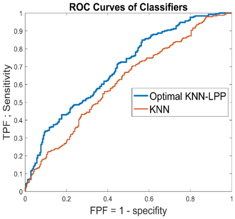
Comparison of two ROC curves generated by the original KNN model using the initial 44 features and the optimal LPP-KNN model using 4 features.

Table 5 summarizes several other parameters or assessment indices commonly computed and used in epidemiology studies to predict breast cancer risk. Using the threshold of (T = 0.5) to divide all testing cases into two risk classes, the odds ratio is 4.60 with a 95% confidence interval of [3.16, 6.70]. The data may indicate that women in the high-risk group have more than 4 times higher short-term breast cancer risk or probability of having or developing mammography-detectable cancer in the next subsequent breast cancer screening, which means 12 to 18 months after the “prior” negative screening of interest, than the women classified in the low risk group.

Table 5.

Odds and Risk Ratio of the proposed KNN-LPP method.

Significance level	95 %
Risk Ratio	1.7597< 2.1519 <2.6316
Absolute risk reduction	36.4%
Relative risk reduction	53.5%
Odds Ratio	3.1568< 4.5997 <6.7021
Phi	0.3600
Critical Odds Ratio (COR)	1.1006

In addition, after dividing 500 testing cases into 5 subgroups of 100 cases based on the LPP-KNN model generated cancer risk prediction scores (as shown in Table 6), the adjusted odd ratios increased from 1.0 in the 1^st baseline subgroup of 100 cases with low risk prediction scores to 11.2 in the 5^th subgroup of 100 cases with the high-risk scores. Regression analysis result also demonstrated an increasing trend of the odds ratios with the increase in LPP-KNN model-predicted risk scores. The slope of the regression trend line between the adjusted odds ratios and the predicted risk scores is significantly different from the zero slope (p < 0.01).

Table 6.

Adjusted ORs and 95 % CIs for five subgroups of cases

Number of Cases (Positive- Negative)	Adjusted OR	95 % CI
23–77	1.00	Reference
49–51	3.21	1.75–5.91
46–54	2.85	1.55–5.24
55–45	4.092	2.22–7.53
77–23	11.20	5.8–21.65

4. DISCUSSION

In this study, we proposed and tested a new approach to develop a computer-aided image processing, quantitative feature analysis and machine learning scheme for predicting short-term breast cancer risk, or the likelihood of women having or developing imaging detectable early breast cancer in the next subsequent mammography screening. This study has a number of unique characteristics compared to the previous studies reported in the literature to help improve efficacy in predicting short-term breast cancer risk and/or eventually establish a more effective personalized breast cancer screening paradigm.

First, as shown in Figure 3(a) and (b), two types of machine leaning methods are commonly applied in medical imaging informatics field to date. The main disadvantage of a conventional machine learning method is requiring many subjectively defined or “handcrafted” image features. Although deep learning (DL) can automatically define DL-generated image features by directly learning from the sample images, which may more effectively define or represent internal structure of image data, training a robust DL model typically requires a very large image dataset. In this study, we tested a third approach, which partially takes advantage of deep learning while also maintains advantage of the conventional machine learning to be trained using a relatively small image dataset. In our approach as shown in Figure 3(c), a LPP-based feature regeneration algorithm was used to automatically learn and generate a small set of new features from a relatively large pool of initially computed image features. This process is different from the conventional feature selection, which selects optimal features from the initial feature pool (i.e., using a sequential forward floating selection (SFFS) feature selection method (Tan et al 2014)). LPP aims to learn and redefine the effective features, which are different from any of the existing image features in the initial feature pool. Our study results demonstrated that using this LPP-based feature regeneration approach enabled us to create a smaller or compact new feature vector and yield higher prediction performance than using either all initial image features or a set of selected highly performed features.

Second, patient age is a well-known breast cancer risk factor with the highest discriminatory power in the existing epidemiology based breast cancer risk models (Amir et al 2010). Our previous studies may have bias by using the datasets in which the average age of women in the higher risk group was significantly higher than the average age in the lower risk group (Zheng et al 2012). In order to overcome this potential bias, we in this study assembled an age-matched image dataset (as shown in Table 1). As a result, we removed a potential biased impact factor. The study result is encouraging by comparing to the previous studies. Specifically, although the highest adjustable odds ratio yielded in this study was very comparable or slightly higher than the results reported in our previous studies (i.e., 11.2 vs. 9.1 (Zheng et al 2014) or 11.1 (Tan et al 2016)), using an age-matched dataset in this study may be important to demonstrate the robustness of developing a new optimal imaging marker based on bilateral asymmetry of mammographic tissue density between the left and right breasts.

Third, although computer-aided image processing and breast cancer risk prediction schemes had been previously developed and tested by different research groups including our own using an “eager” machine learning methods or models (i.e., artificial neural network and support vector machine), we in this study also tested a “lazy” learning method using a KNN algorithm for the purpose of predicting short-term breast cancer risk. Our study results showed that KNN can be used not only to predict cancer risk, but also to yield higher prediction accuracy that an optimized SVM model using the same testing dataset and cross-validation method. This result is quite interesting and may be worth further investigation. Using a local instance based learning method (i.e., a KNN algorithm) can provide great flexibility to develop a new machine learning based imaging marker or prediction mode because it will be relatively easy to periodically add new image data to increase size and diversity of the reference database for the instance-based learning model, without a complicated retraining to produce a global optimization function, which is required by all other “eager” learning methods (Park et al 2007, Wang et al 2017).

In addition, we can also make a number of potentially interesting observations from our experimental results. For example, the highest AUC value using all 44 features was 0.62. While keeping K = 5 in the KNN learning model, removing 34 lower performed features enabled an increase of AUC value by 3.2% from 0.62 to 0.64. Furthermore, when adopting a LPP-KNN model using 4 LPP-regenerated features, AUC increased to 0.68 (representing a 9.7% increase). Thus, the results confirmed that although a large number of image features can be initially computed, removing lower performed and redundant features, as well as generating more effective features, played an important role to increase performance of multi-feature fusion based machine learning models. Applying LPP does not only reduce the dimension of feature space, but also it is able to reorganize the new feature vector to achieve lower amount of redundancy and maximum variance. Hence, LPP-regenerated feature vector represents an optimal combination of the highly effective parts of all input features.

Fourth, although the size of our dataset is limited to 500 or 250 per class, applying the LPP feature regeneration approach also helped to increase the robustness of the testing result. Specifically, using the LPP approach increased the ratio between the training cases per class and image features from original 5.7 (250/44) using all 44 features in the initial feature pool to 62.5 (250/4) using only 4 LPP-regenerated features. Thus, based on the machine learning theory, increasing this ratio will increase the robustness of the machine learning classifier to reduce the risk of overfitting. In addition, we used a leave-one-case-out (LOCO) cross-validation method to train and test the classifier, which also eliminates the bias of case partition or selection.

Despite the encouraging results, this is a proof-of-concept type study with several limitations, which needs to be addressed and/or overcome in future studies. First, although LPP is able to regenerate an optimal image feature vector, its ultimate performance depends on the quality of initial feature pool. The initial feature pool with 44 features used in this study may not have been an optimal feature pool. Thus, we will continue our efforts to improve the computer-aided image processing scheme to more accurately and robustly segment dense mammographic tissue regions and compute image features. Second, due to the potential compression difference between left and right breasts, breast sizes and density overlapping ratio (or pixel values) depicting on two bilateral images may not be the same. In order to reduce the potential errors in computing feature difference, we need to continue investigating new methods to compensate the difference and reduce the errors. Third, since the regions near breast skin and behind chest wall have high pixel values in mammograms, in order to avoid adding them into the dense fibro-glandular tissue volume, we need to develop a more accurate method to automatically remove these regions without losing significant information of breast area. Fourth, it is also important to more effectively detect and compensate other types of image noise, which may exist and vary in screening mammograms due to the variety of technical issues in conducting mammography examinations on different individual women. The goal is to develop a more robust computer-aided image processing scheme to achieve high accuracy in mammographic dense tissue segmentation. Last, this study only used and analyzed images acquired from one “prior” mammography screening. In the future studies, we will collect more cases with multiple “prior” mammography screenings and investigate the feasibility of improving performance of short-term breast cancer risk prediction by combining the image feature variation trend among the multiple mammography screenings into the risk prediction models.

References

- Aghaei F, Tan M, Hollingsworth AB, Zheng B. Applying a new quantitative global breast MRI feature analysis scheme to assess tumor response to chemotherapy. J Magn Reson Imaging. 2016;44:1099–1106. doi: 10.1002/jmri.25276. [DOI] [PMC free article] [PubMed] [Google Scholar]
- Amir E, Freedman OC, Seruga B, Evans DG. Assessing women at high risk of breast cancer: a review of risk assessment models. J Natl Cancer Inst. 2010;102:680–691. doi: 10.1093/jnci/djq088. [DOI] [PubMed] [Google Scholar]
- Berlin L, Hall FM. More mammography muddle: emotions, politics, science, cost and polarization. Radiology. 2010;255:311–316. doi: 10.1148/radiol.10100056. [DOI] [PubMed] [Google Scholar]
- Berg WA, Campassi C, Langenberg P, Sexton MJ. Breast imaging reporting and data system: Inter- and intra-observer variability in feature analysis and final assessment. Am J Roentgenol. 2000;174:1769–1777. doi: 10.2214/ajr.174.6.1741769. [DOI] [PubMed] [Google Scholar]
- Brawley OW. Risk-based mammography screening: an effort to maximize the benefit and minimize the harms. Ann Intern Med. 2012;156:662–663. doi: 10.7326/0003-4819-156-9-201205010-00012. [DOI] [PubMed] [Google Scholar]
- Carney PA, Miglioretti DL, Yankaskas BC, et al. Individual and combined effects of age, breast density, and hormone replacement therapy use on the accuracy of screening mammography. Ann Intern Med. 2003;138:168–175. doi: 10.7326/0003-4819-138-3-200302040-00008. [DOI] [PubMed] [Google Scholar]
- Damases C, Brennan PC, Mello-Thoms C, McEntee MF. Mammographic breast density assessment using automated volumetric software and breast imaging reporting and data system (BIRADS) categorization by expert radiologists. Acad Radiol. 2016;23:70–77. doi: 10.1016/j.acra.2015.09.011. [DOI] [PubMed] [Google Scholar]
- Gail MH, Brinton LA, Byar DP, et al. Projecting individualized probabilities of developing breast cancer for white females who are being examined annually. J Natl Cancer Inst. 1989;81:1879–1186. doi: 10.1093/jnci/81.24.1879. [DOI] [PubMed] [Google Scholar]
- Gail MH, Mai PL. Comparing breast cancer risk assessment models. J Natl Cancer Inst. 2010;102:665–668. doi: 10.1093/jnci/djq141. [DOI] [PubMed] [Google Scholar]
- He X, Niyogi P. Locality preserving projections. Advances in neural information processing systems. 2004:153–160. [Google Scholar]
- Hubbard RA, Kerlikowske K, Flowers CI, et al. Cumulative probability of false-positive recall or biopsy recommendation after 10 years of screening mammography: a cohort study. Ann Intern Med. 2011;155:481–492. doi: 10.1059/0003-4819-155-8-201110180-00004. [DOI] [PMC free article] [PubMed] [Google Scholar]
- Kopans DB. Basic physics and doubts about relationship between mammographically determined tissue density and breast cancer risk. Radiology. 2008;246:348–353. doi: 10.1148/radiol.2461070309. [DOI] [PubMed] [Google Scholar]
- Leng Y, Xu X, Qi G. Combining active learning and semi-supervised learning to construct SVM classifier. Knowledge-Based Systems. 2013;44:121–131. [Google Scholar]
- Li Q, Doi K. Reduction of bias and variance for evaluation of computer-aided diagnosis schemes. Med Phys. 2006;33:868–875. doi: 10.1118/1.2179750. [DOI] [PubMed] [Google Scholar]
- Mitchell TM. Machine learning. WCB McGraw-Hill; Boston, MA: 1997. [Google Scholar]
- Narol SA, Sun P, Wall C, et al. Impact of screening mammography on mortality from breast cancer before age 60 in women 40 to 49 years of age. Curr Oncol. 2014;21:217–221. doi: 10.3747/co.21.2067. [DOI] [PMC free article] [PubMed] [Google Scholar]
- Park SC, Sukthankar R, Mummert L, et al. Optimization of reference library used in content-based medical image retrieval scheme. Med Phys. 2007;34:4331–4339. doi: 10.1118/1.2795826. [DOI] [PMC free article] [PubMed] [Google Scholar]
- Saslow D, Boetes C, Burke W, et al. American cancer society guidelines for breast cancer screening with MRI as an adjunct to mammography. CA Cancer J Clin. 2007;57:75–89. doi: 10.3322/canjclin.57.2.75. [DOI] [PubMed] [Google Scholar]
- Shen D, Wu G, Suk HI. Deep learning in medical image analysis. Annu Rev Biomed Eng. 2017;19:221–248. doi: 10.1146/annurev-bioeng-071516-044442. [DOI] [PMC free article] [PubMed] [Google Scholar]
- Tan M, Pu J, Zheng B. Optimization of breast mass classification using sequential forward floating selection (SFFS) and a support vector machine (SVM) model. Int J Comput Assist Radiol Surg. 2014;9:1005–1020. doi: 10.1007/s11548-014-0992-1. [DOI] [PMC free article] [PubMed] [Google Scholar]
- Tan M, Zheng B, Leader JK, Gur D. Association between changes in mammographic image features and risk for near-term breast cancer development. IEEE Trans Med Imaging. 2016;35:1719–1728. doi: 10.1109/TMI.2016.2527619. [DOI] [PMC free article] [PubMed] [Google Scholar]
- Tyrer J, Buffy SW, Cuzick J. A breast cancer prediction model incorporating familial and personal risk factors. Stat Med. 2004;23:1111–1130. doi: 10.1002/sim.1668. [DOI] [PubMed] [Google Scholar]
- Van Ziteren M, van der Net JB, Kundu S, et al. Genome-based prediction pf breast cancer risk in the general population: a modeling study based on meta-analyses of genetic associations. Cancer Epidemiol Biomarkers Prev. 2011;20:9–22. doi: 10.1158/1055-9965.EPI-10-0329. [DOI] [PubMed] [Google Scholar]
- Wang X, Lederman D, Tan J, et al. Computerized prediction of risk for developing breast cancer based on bilateral mammographic breast tissue asymmetry. Med Eng Phys. 2011;33:934–942. doi: 10.1016/j.medengphy.2011.03.001. [DOI] [PMC free article] [PubMed] [Google Scholar]
- Wang Y, Aghaei F, Zarafshani A, et al. Computer-aided classification of mammographic masses using visually sensitive image features. J Xray Sci Technol. 2017;25:171–186. doi: 10.3233/XST-16212. [DOI] [PMC free article] [PubMed] [Google Scholar]
- Wei J, Chan HP, Wu YT, et al. Association of computerized mammographic parenchymal pattern measure with breast cancer risk: a pilot case-control study. Radiology. 2011;260:42–49. doi: 10.1148/radiol.11101266. [DOI] [PMC free article] [PubMed] [Google Scholar]
- Weinberger KQ, Saul LK. Distance metric learning for large margin nearest neighbor classification. Journal of Machine Learning Research. 2009;10:207–244. [Google Scholar]
- Yan S, Qian W, Guan Y, Zheng B. Improving lung cancer prognosis assessment by incorporating synthetic minority oversampling technique and score fusion method. Med Phys. 2016;43:2694–2703. doi: 10.1118/1.4948499. [DOI] [PubMed] [Google Scholar]
- Zheng B, Chang Y-H, Gur D. Computerized detection of masses in digitized mammograms using single image segmentation and a multi-layer topographic feature analysis. Acad Radiol. 1995;2:959–966. doi: 10.1016/s1076-6332(05)80696-8. [DOI] [PubMed] [Google Scholar]
- Zheng B, Lu A, Hardesty LA, et al. A method to improve visual similarity of breast masses for an interactive computer-aided diagnosis environment. Med Phys. 2006;33:111–117. doi: 10.1118/1.2143139. [DOI] [PubMed] [Google Scholar]
- Zheng B, Sumkin JH, Zuley ML, et al. Bilateral mammographic density asymmetry and breast cancer risk: A preliminary assessment. Eur J Radiol. 2012;81:3222–3228. doi: 10.1016/j.ejrad.2012.04.018. [DOI] [PMC free article] [PubMed] [Google Scholar]
- Zheng B, Tan M, Ramalingam P, Gur D. Association between computed tissue asymmetry in bilateral mammograms and near-term breast cancer risk. Breast J. 2014;20:249–257. doi: 10.1111/tbj.12255. [DOI] [PMC free article] [PubMed] [Google Scholar]