

Abstract
Studies on interactions between brain regions estimate effective connectivity, (usually) based on the causality inferences made on the basis of temporal precedence. In this study, the causal relationship is modeled by a multi-layer perceptron feed-forward artificial neural network, because of the ANN’s ability to generate appropriate input–output mapping and to learn from training examples without the need of detailed knowledge of the underlying system. At any time instant, the past samples of data are placed in the network input, and the subsequent values are predicted at its output. To estimate the strength of interactions, the measure of “Causality coefficient” is defined based on the network structure, the connecting weights and the parameters of hidden layer activation function. Simulation analysis demonstrates that the method, called “CREANN” (Causal Relationship Estimation by Artificial Neural Network), can estimate time-invariant and time-varying effective connectivity in terms of MVAR coefficients. The method shows robustness with respect to noise level of data. Furthermore, the estimations are not significantly influenced by the model order (considered time-lag), and the different initial conditions (initial random weights and parameters of the network). CREANN is also applied to EEG data collected during a memory recognition task. The results implicate that it can show changes in the information flow between brain regions, involving in the episodic memory retrieval process. These convincing results emphasize that CREANN can be used as an appropriate method to estimate the causal relationship among brain signals.
Keywords: Effective connectivity, Multi-layer perceptron artificial neural network, Multivariate autoregressive, Causality, Memory recognition
Introduction
Effective connectivity is one of the areas of technical advancement in neuroscience researches that is widely used for better understanding the interactions between brain regions, and the influences neural structures exert on one another (Friston 1994; Horwitz 2003; Stam and Reijneveld 2007). The connectivity based models can produce behavior, which is an essential requirement for any neural model of cognition (van der Velde and de Kamps 2015). Estimation of effective connectivity supports the inference of causal relationships and directional information flow, and may provide insights into the interactive dynamics in normal (Astolfi et al. 2005; Bitan et al. 2005; Kundu et al. 2013; Wang and Zhu 2016; Zeng et al. 2016) or disordered (Baccala et al. 2004; Behnam et al. 2008; Cadotte et al. 2009; Coben et al. 2013, 2014; Gravier et al. 2016; Kundu et al. 2013; Liu et al. 2012; Protopapa et al. 2016) brain functions. Among many definitions of causality (Atmanspacher and Rotter 2008), there are two important aspects that are of practical relevance: (1) temporal precedence: causes precede their consequences; (2) physical influence: manipulation of the causes changes their consequences (Valdes-Sosa et al. 2011). In this study, like most of the time-series analysis of the causal inference, the first aspect of temporal precedence is considered.
Among various methods for estimating effective connectivity from electrophysiological (EEG or MEG) or neuroimaging (fMRI) data [reviewed in Lehnertz (2011)], those based on Multivariate Autoregressive (MVAR) models have been widely and effectively used for studying brain connectivity (Brunet et al. 2011; Cheung et al. 2012; Faes and Nollo 2010). The classical forms of these models represent the interaction between brain regions in the form of linear difference equations (Astolfi et al. 2008; Omidvarnia et al. 2014).
Unlike the Dynamic Causal Model (DCM) (Friston et al. 2003) or Structural Equation Model (SEM) (Astolfi et al. 2005), MVAR models do not require any prior anatomical model and/or physiological information. In addition, in contrast to Dynamic Bayesian Network (DBN) models which consider only one previous sample of data for estimating the causal relationship (Burge et al. 2009; Rajapakse and Zhou 2007; Wu et al. 2012), the MVAR models investigate the effective connectivity using data with more time lags. Considering more time lags may improve inferences about temporal causality between brain regions and provide better insight into its dynamics. This is especially important for the brain phenomena in which different neural ensembles activate in sequence over time to compose the flow of information [for example, in memory retrieval (Ashby et al. 2005; McIntosh 1999), epilepsy (Addis et al. 2007; Cadotte et al. 2009; McIntosh 1999), etc.]
Beside the advantages mentioned above, there are some important issues that should be taken into account when effective connectivity is estimated using MVAR models. First of all, processes in the brain are usually within a dynamic framework with highly interactive brain regions (Wennekers and Ay 2005), which implies that an efficient model should track the changes in casual relationships over time. With estimating a unique MVAR model on an entire time interval, transient pathways of information flow remain hidden (Astolfi et al. 2008). This limitation may bias the physiological interpretation of the results obtained by the connectivity technique employed (Hemmelmann et al. 2009). This has prompted the development of time-varying MVAR-based effective connectivity measures [e.g. time-varying Granger causality (Hesse et al. 2003), time-varying Partial Directed Coherence (PDC) (Omidvarnia et al. 2014; Sommerlade et al. 2009), and Directed Transfer Function (DTF) (Astolfi et al. 2008)] for EEG signal processing. These methods, however, require a sufficient signal-to-noise ratio (SNR) to produce reliable results (Omidvarnia et al. 2014). Therefore, there is a need for an appropriate method to overcome these challenges and to represent effective connectivity changes over time with an acceptable performance for a wide range of SNRs (Astolfi et al. 2007)
Artificial Neural Networks (ANNs) have some distinguishing features that make them valuable and attractive for being a (linear/nonlinear) multivariate autoregressive model. They are data-driven, nonlinear and adaptive methods, which do not require any prior assumption of the model for the problem under study. They are able to generate an appropriate mapping between their inputs and outputs. By assuming that in the ANN, the interconnected neurons, which exchange messages between each other, may be a simplified simulation of the way in which brain regions interact with each other, one can exert the network to encode the brain regions connectivity.
Relying on the advantages of ANNs, McNorgan and Joanisse (2014) introduced a computational model for investigation of cortical connectivity from resting state fMRI data. Their model encoded activation co-occurrence probabilities within the data, and estimated the cortical connectivity in terms of inter-regional network weights.
The present study tries to estimate the effective connectivity by implementing the MVAR modelling with a Multi-Layer Perceptron (MLP) neural network. We call the method “Causal Relationship Estimation by Artificial Neural Network (CREANN)”, and investigate its ability in estimating effective connectivity and tracking interaction changes over time. Furthermore, as the performance of MVAR model based methods is affected by some general factors such as the signal-to-noise ratio (SNR) and the choice of the correct model order (Astolfi et al. 2006), these parameters are tested in assessing the effective connectivity of simulated data by CREANN method. The effectiveness of the method on real (EEG) data is illustrated by showing changes in effective connectivity during a memory retrieval task.
This paper is organized in four parts. The “Method” section gives an overview of the structure of the MVAR model, MLP learning and Causality coefficient (Cc) measure, and provides a brief description of the time-varying CREANN method. In the “Result” section, we first apply the method on two simulated models, including time-invariant and time-varying coefficients. The performance of the proposed method in the presence of different noise levels, different model orders, and different shapes of time-varying coefficients is evaluated by simulated data. Then, the method is applied on EEG data collected in a visual memory recognition task. The result has been reported in last part of the “Result” section, and finally they are discussed in the “Discussion” section.
Method
Suppose we have M time series of length L, representing samples of cortical signals from M regions of interest (ROI). Let be the nth sample of the time series with (L − p) number of samples (n = p + 1, …, L), and
| 1 |
be the vector of p past samples of (M) multivariate time series. One can assume that at time n, is generated by a general MVAR model:
| 2 |
which can be linear or nonlinear, quantitatively describes the cortical interaction between the signals, and is a normally distributed real-valued zero-mean white noise vector with diagonal covariance matrix R. For the case of linear assumption for dependencies between the regions, the Eq. (2) turns into the classical linear MVAR model. Although this assumption may not possibly represent all the characteristics of brain dynamics, for simplification of the computations, in this study (like many studies on effective connectivity (Astolfi et al. 2006; Ghasemi and Mahloojifar 2012; Giannakakis and Nikita 2008; Winterhalder et al. 2005)) the linear dependencies have been assumed for simulated models.
Multivariate autoregressive model
For a given time series, a multivariate autoregressive (MVAR) model of order p is defined as (Hytti et al. 2006):
| 3 |
the matrix is given by
| 4 |
for d = 1, …, p. The real-valued coefficient is the weighting factor that characterizes the contribution of x j(n − d) to x i(n).
Independence between a pair of signals results in a (near) zero coefficient () while dependence is reflected in a nonzero magnitude. High coefficients indicate strong “effective connectivity”.
ANN as a multivariate autoregressive model
Artificial neural networks are inspired by the structure and functionality of the human brain. Because of nonlinear signal processing, the capability of being a universal approximator, and no prerequisite of detailed knowledge about the problem, ANNs have become an attractive option to serve as a nonlinear multivariate autoregressive model (Bressler et al. 2007). They have, therefore, the potential to represent the interaction between different brain regions. If the model’s inputs and outputs are selected properly, extracting information from the model by suitable criteria could provide a good explanation for what has happened within the underlying (brain) system.
For the problem of estimating the effective connectivity, the neural network input nodes are the lagged samples of the M time series at different delays, i.e. where p is the maximum time-lag considered for the signals. During training through time, the network tries to predict the next samples , as its output, based on previous samples in input nodes. A schematic representation of this procedure is shown in Fig. 1.
Fig. 1.

a A typical effective connectivity map. There are M regions of interest (ROI). The causal effects are not necessarily the same for each pair channel. b CREANN model: a feed-forward neural network for modeling the interaction between these M regions. Here the M signals with lagged samples are feeding the network’s input. During the training, the subsequent samples, as the network’s outputs, are predicted based on previous samples of all regions. This produced a nonlinear MVAR model which information about its coefficients is embedded in the network’s parameters
After training the network, the major issue is to find causal relationships between network’s inputs (past activities of one region) and outputs (subsequent activities of the others). In other words, we want to estimate the parameters of this MVAR model. We looked for some measures to be large (small) when the network’s inputs have strong (weak) effects on the outputs. For this purpose in this study, we define “Causality coefficient” (Cc) to make a relation between network’s inputs and outputs based on the network’s parameters.
The Causality coefficient
To extract information from the trained network, let’s take a look to its structure. For a network with N i inputs, one hidden layer with N h (nonlinear) neurons, and N o (linear) output units, we have
| 5 |
where z k is the induced local field of the kth hidden unit, and w qk is the weight value between the kth hidden unit and the qth input node (x q). The nonlinear activation function of the kth hidden neuron is defined as
| 6 |
a k and are the scaling parameters of the well-known hyperbolic tangent function , which are adapted during the training. The network output is
| 7 |
where v kl is the weight value between the lth output neuron and the kth unit in the hidden layer.
If the nonlinear function is approximated by its first term of Taylor series, then we have
| 8 |
Therefore, the Causality coefficient (Cc), which relates the network inputs to its outputs, is defined as
| 9 |
Cc lq represents the influence of qth input node on the lth output neuron. It seems that the Causality coefficient, compared to the previously defined measure of “multiplying the network weights ()”, has a stronger mathematical basis. Multiplying the network weights has been previously used for rule extraction of ANN (Baba et al. 1990; Boger and Guterman 1997; Saad and Wunsch II 2007).
Since in this study, the network input nodes are delayed samples of time series, and the outputs are subsequent samples of all signals, the Causality coefficient (Cc) explains the relationship between the past and future of the signals and represents temporal causality (effective connectivity) between regions. If we put all the coefficients in a matrix, we can achieve the Causality matrix () as:
| 10 |
M is the number of time series of the ROIs, and p is the maximum lag of the signals. The shows the causal effect of x j(n − d) on x i(n), which is comparable with the classic MVAR coefficient (c.f. “Multivariate autoregressive model” section). The notable point about the matrix is that it is not symmetric, and .
For more convenience, in the rest of paper, we use symbol instead of Cc lq., because it clearly shows the delay d.
Applying CREANN
Before starting network training, we should note that the effectiveness of neural network models and their performance in forecasting time series events is usually influenced by the parameters of the model, such as the number of input nodes, number of hidden layers and hidden neurons in each layer, and the choice of the learning algorithm and transfer functions. These parameters are problem dependent and often require trial and error in order to find the best model for a particular application.
Input selection (choice of model order)
In particular, the “input selection” is an important required step in exploring the effective connectivity among large numbers of recorded signals in neuroimaging. This term refers to a procedure for selecting the minimum number of all available inputs (signals) that have maximum relevance to a specific output (signal). If an ANN is seen as a MVAR model, the appropriate number of time lags of the input signals would be identical to the optimal model order and one can find it using traditional order selection criteria such as Akaike Information Criterion (AIC) and Schwarz’s Bayesian Criterion (SBC) (Cheung et al. 2012; Neumaier and Schneider 2001). For a reliable estimation of the MVAR parameters, the signal length (L) should be much longer than Mp (Hytti et al. 2006).
On the other hand, with the view of function approximation, various methods have been recently proposed for the development of appropriate ANN’s input selection. For example, some information theoretic based measures has been used for this issue (Bowden et al. 2005; May et al. 2008; Sharma 2000). In this study, we use mutual information (MI) technique for estimating the optimum time lag. The MI for every pair of x i(n) and x j(n − d) is computed (for d = 1 up to a pre-defined Max_lag). Then MI(d) is plotted as a function of delay (d). The optimum lag p opt is the minimum d when the steepness of the decline slope of MI(d) becomes almost negligible and the curve becomes flat (Fig. 2). This point on the MI graph shows that the lagged signal x j(n − (p opt + 1)) does not have adequate information shared with for being involved in prediction it. In this study, the average p opt, estimated from MI(d) curves, along with the SBC criterion is used for estimating optimal model order (time lag).
Fig. 2.

Calculating mutual information (MI) for estimating optimum model order. Here p opt is marked with a circle. It is the minimum delay (d) when MI curve starts to become flat
Network structure and learning algorithm
Adjusting appropriate network structure for the application is widely determined by trial and error. A full description of ANN structure optimization is beyond the scope of this investigation, and in this study, the network architecture is set by trial and error. Only one hidden layer is considered for the network. For simulated data, we varied the number of hidden neurons (N h) from N h = N o to N h = 3N i ( is the number of output and input nodes, respectively). As the training and testing error did not significantly improve by increasing the number of hidden neurons, we set N h = N o in all simulations.
The training algorithm is gradient descent error backpropagation (EBP) with momentum (α) and adaptive learning rate (η). The parameters are updated after each input is applied to the network.
Estimating time invariant/time-varying coefficients
For assessment of average (overall) causal relationship between signals, one can suppose that MVAR model coefficients are time invariant, and estimate a unique MVAR model for the total lengths of the signal. In the case of time-invariant coefficient estimation, the neural network should be trained by all data points, and the corresponding parameters would be considered for computing Causality coefficients in the next step. However, this overall estimation of effective connectivity may not provide adequate information for better understanding the dynamics of the interactive brain regions. To overcome this limitation and for representing changing causal relationships between cortical areas through time, time-varying MVAR modeling (tv-MVAR) has been recently proposed by researchers (Giannakakis and Nikita 2008; Hesse et al. 2003; Omidvarnia et al. 2014). In the present study, data windowing technique is used for estimating time-varying effective connectivity. Data is divided into some non-overlapping segments, with the proper window length. For considering appropriate window length, there is a tradeoff between the likelihood of stationarity (shorter is better) and accuracy of model fit (longer is better). The ANN is applied to each data segment, and the causality matrix is computed for every segment. The “time-varying CREANN” (tv-CREANN) method is described as follows.
Preparation: Define model order and set the network architecture, i.e. the number of hidden neurons, initial training parameters , momentum coefficient (α), and initial learning rate (). and are the initial input/hidden and hidden/output weight matrix, respectively. are the vectors of (trainable) parameters of hidden activation function (). The initial parameters are chosen randomly.
Initialization: All data points are used for training the network (this provides a general estimation of the network parameters corresponding to the data characteristics). The parameters of this trained network () are utilized as initial training parameters for the next step.
Updating parameters for data segments: in the next step the data points are divided into N non-overlapping segments. For each segment 90% of first data points are considered as training and the last 10% as testing data For each segment a network is trained with initial parameters produced by previous segment (for the first segment, the initial parameters were those computed in the ‘initialization’ step).
Computing causality matrix : The Causality coefficients for each segment are estimated by Eqs. (9), (10).
The updating step repeats for all data segments and the corresponding coefficients are estimated sequentially. Table 1 is the pseudo code for the tv-CREANN method. A typical time-varying Causality coefficient estimation procedure is depicted in Fig. 3.
Table 1.
Pseudo code for tv-CREANN method

Fig. 3.
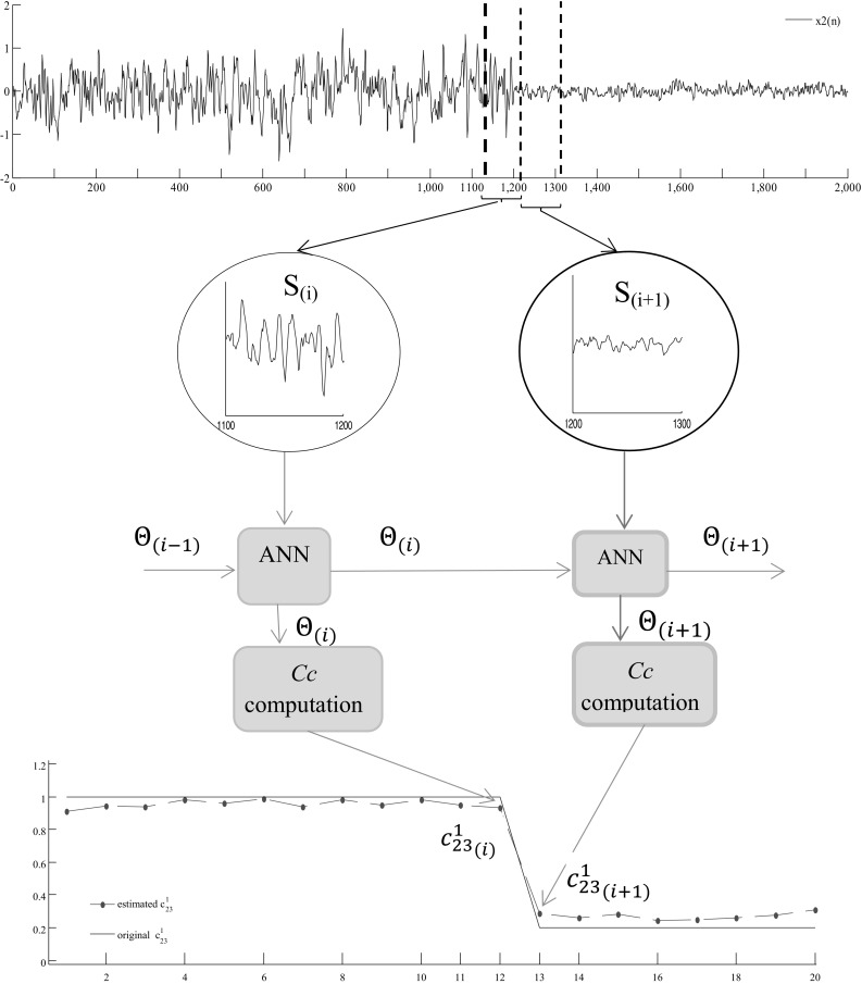
The time-varying CREANN (tv-CREANN) for estimating effective connectivity. Here is an example of estimating time-varying MVAR coefficient for simulated model. (Top): the time series. (Middle): the tv-CREANN technique; ; , where are Input/Hidden and Hidden/Output network weights, and are the vector parameters of hidden activation function for segment S (i), respectively. (Bottom): the coefficient which is the influence of x 3(n − 1) on x 2(n). Estimated coefficient is showed by red dashed line, and original is depicted by blue solid line. (Color figure online)
Validation the model
Beside all modeling efforts, it is important to evaluate the accuracy of the proposed method before it can be analyzed and interpreted in future effective connectivity assessments. Here, the validation factors to determine the model adequacy fall into three parts. First, the designed network should have acceptable training error, showing its ability to follow the time series under study by changing the ANN’s parameters (i.e. the connecting weights, , and activation function’s parameters ). Second factor is forecasting accuracy, the ability of the model to synthesize time series for testing samples of data. The testing error must be in the range of the training error, indicating the appropriate generalization ability for the network. The training and testing errors are the root mean squared error (RMS) between actual (target) and predicted (network output) values of the time series. The third validation factor is defined from the standard MVAR modeling point of view, which is based on their residuals. Residuals show an indication of remaining un-modeled structures in the data. The residuals for an acceptable validated model should be approximately equal to the white noise (Chuang et al. 2012; Hill et al. 2012). We use these factors for validating our model, and the results are presented in the following section.
Result
In this section, first the simulated data are presented to evaluate the performance of our proposed method in estimating the effective connectivity when the true MVAR coefficients is known. Then it applied on the EEG data recorded in a recognition memory task.
Simulation
Two independent simulations are conducted covering both time-invariant and time-varying circumstances. The effect of choice of model order and the level of noise on the method’s performance, and its ability for tracking various changes in coefficients is evaluated by simulated data in the following sections.
Simulated model with time-invariant coefficients
In this case, the simulated data is obtained from a three dimensional MVAR model with time-invariant coefficients:
| 11 |
is white Gaussian noise. In the case of time invariant model coefficients (which is a simulation of overall causal relationship), a single MVAR model is fitted to all data points (entire length of signals). The network input is fed by lagged samples of the data, and the subsequent sample is predicted during training the network. Table 2 contains the estimated time invariant coefficients of the MVAR model.
Table 2.
Original (italics) and estimated coefficients in the case of time-invariant model coefficients
| x1(n − 1) | x1(n − 2) | x2(n − 1) | x2(n − 2) | x3(n − 1) | x3(n − 2) | |||||||
|---|---|---|---|---|---|---|---|---|---|---|---|---|
| Original | Estimated | Original | Estimated | Original | Estimated | Original | Estimated | Original | Estimated | Original | Estimated | |
| x1(n) | 0.500 | 0.522 | −0.700 | −0.704 | −0.600 | −0.421 | 0.000 | 0.021 | 0.000 | 0.000 | 0.000 | 0.004 |
| x2(n) | 0.200 | 0.205 | 0.000 | −0.001 | 0.700 | 0.710 | −0.500 | −0.506 | 0.800 | 0.528 | 0.000 | 0.013 |
| x3(n) | 0.000 | −0.017 | 0.000 | −0.002 | 0.000 | −0.012 | 0.000 | −0.009 | 0.800 | 0.824 | 0.000 | −0.002 |
is 0.104
To evaluate the performance of the CREANN method in estimating effective connectivity (in the form of MVAR coefficients), the root mean square (RMS) of the estimating error is computed as (Tuncer et al. 2012):
| 12 |
where . is the number of total coefficients, c (estimated)q is the coefficient estimated by the CREANN method, and c (original)q is the original coefficient in the simulated model.
The RMS error for time-invariant coefficient estimation is 0.104. The values of Table 2 also show that the CREANN can provide a sufficient approximation of these coefficients.
Simulated model with time-varying coefficients
For the case of time-varying coefficients, the previous MVAR model is modified as:
| 13 |
where is the influence of x 2(n − 1) on x 1(n), and is the effect of x 3(n − 1) on x 2(n), described as follows (L is length of simulated data and for this study L = 2000):
| 14 |
Here we divide the data into N = 20 non-overlapping segments, and apply the tv-CREANN method (the procedure is described in previous section and schematically is depicted in Fig. 3). By choosing N = 20, the data segment length is close to 100 points ((L − p)/N). Considering the number unknown parameters in the neural network, this data length seems to be large enough to be used by the ANN.
For comparing Causality coefficient with the measure of multiplying the network weights, we iterate performing the tv-CREANN on simulated time-varying model for 9 times, with different random initial network parameters (). The RMS error for estimating all coefficients (RMS estimation), and the average variance () of estimating all time-invariant coefficients for the nine times iterating the procedure are presented in Table 3. Furthermore, Fig. 4 shows the time-varying coefficients and estimated by these two measures.
Table 3.
comparison of estimation results produced by Causality coefficient and the measure of multiplying the network weights
| Causality coefficient | Multiplying the network weights | |
|---|---|---|
| RMS estimation | 0.113 | 0.326 |
| 0.004 | 1.624 |
Fig. 4.

Estimation results of time-varying coefficients [] for two methods. Original results are shown by solid lines and estimated coefficients by Causality coefficient (shown by a*b*V*W) are depicted by red dashed lines, while estimated coefficients by multiplying the network weights (shown by V*W) are depicted by blue dotted lines. (Color figure online)
The left panel shows the original coefficient , which changes slowly as a triangle function, and the corresponding estimated by Causality coefficient could acceptably follow the changes. The right panel of Fig. 4 shows the original value of , which changes quickly (as a step function), and estimated coefficient , tracking this sudden change with a slight delay. Since the length of each segment is close to 100 points, the tvCREANN can follow changes with a maximum of 100 point delay. It is obvious that a shorter segment length leads to tracking the changes faster, but as is said before, for the ANN to work properly and for reliable estimation of coefficient values, a relatively sufficient data length is required, which is proportional to the number of unknown parameters of the ANN. The larger length, of course, would reduce the speed of following changes over time.
The results of Table 3 and Fig. 4 clearly reveal that estimation by Causality coefficient is more accurate (with less RMS error), and shows significantly less estimation variance than the method of multiplying the network weights. Therefore, for the rest of paper, we just present the result of the Causality coefficient method.
Figure 5 shows the coefficients corresponding to the variable x2, including time-varying coefficient and other time invariant coefficients. As is obvious, the time-invariant coefficients have small changes in time. Their estimation results are shown by mean and Standard Deviation (SD) of estimation in Table 4.
Fig. 5.

Estimation of coefficients for x2(n) . Estimated results are shown by solid lines and original coefficients are shown by dashed (or dotted) lines. The SNR of simulated data is −20 dB and the RMS error for estimating coefficients is 0.116
Table 4.
Estimation Causality coefficients for time-varying coefficients of the TV-MVAR model
| X1(n − 1) | X1(n − 2) | X2(n − 1) | X2(n − 2) | X3(n − 1) | X3(n − 2) | |||||||
|---|---|---|---|---|---|---|---|---|---|---|---|---|
| Original | Estimated | Original | Estimated | Original | Estimated | Original | Estimated | Original | Estimated | Original | Estimated | |
| X1(n) | 0.5 | 0.57 ± 0.05 | −0.7 | −0.73 ± 0.05 | 0.0 | 0.02 ± 0.05 | 0.0 | −0.10 ± 0.04 | 0.0 | 0.06 ± 0.04 | ||
| X2(n) | 0.2 | 0.23 ± 0.06 | 0.0 | −0.03 ± 0.03 | 0.70 | 0.77 ± 0.12 | −0.5 | −0.45 ± 0.06 | 0.0 | 0.00 ± 0.03 | ||
| X3(n) | 0.0 | −0.03 ± 0.04 | 0.0 | 0.11 ± 0.08 | 0.00 | −0.01 ± 0.01 | 0.0 | −0.06 ± 0.06 | 0.8 | 0.77 ± 0.09 | 0.0 | 0.07 ± 0.08 |
Original coefficients are italics. Estimated time-invariant coefficients are shown by “Mean ± SD*”. In this case, the RMS error for coefficient estimation is 0.116
* Standard deviation
Effect of model order selection on estimation results
As previously described, one can estimate the optimal order of the model using Akaike information criterion and Schwarz’s Bayesian Criterion (SBC). However AIC criterion is known to suffer from over-fitting, because of its tendency to select models with relatively greater orders than the optimal model order (Broman and Speed 2002; Shibata 1984; Stoica and Selen 2004), and SBC have limitations in encountering non-stationary time series (Hannart and Naveau 2012; Zhang and Siegmund 2007).
For evaluating ANN’s capability in estimating coefficients with unknown actual model order, additional lagged samples are considered (Max-lag is greater than p opt), and the network is trained by this new input vector. Here the number of hidden neurons is equal to the number of outputs, and learning rate η and momentum coefficient α are the same for all situations.
The simulation results for the case of the tv-MVAR model show that even if the network’s input is fed by samples with time lag more than p opt, the resulted Cc measures for those samples with Max-lag more than p opt, are very small and close to zero. RMS estimation for different maximum time lags (Max-lag) are shown in Fig. 6 and Table 5.
Fig. 6.

Effect of the assumed order for the MVAR model (maximum time lag) on the estimation error. Changing the model order from 2 to 7 causes only 6% change in the estimation error
Table 5.
Training, testing and RMS error for estimation coefficients in different Max-lag (the hypothesized model order P’)
| p opt = 2 | Max-lag = 2 | Max-lag = 3 | Max-lag = 4 | Max-lag = 5 | Max-lag = 6 | Max-lag = 7 |
|---|---|---|---|---|---|---|
| Training error | 0.182 | 0.180 | 0.181 | 0.179 | 0.176 | 0.177 |
| Testing error | 0.177 | 0.206 | 0.194 | 0.184 | 0.214 | 0.196 |
| RMS estimation | 0.116 | 0.119 | 0.114 | 0.112 | 0.116 | 0.119 |
Effect of noise level on estimation results
To illustrate the effectiveness and performance attributes of our proposed method, several examples of simulated data are generated at various SNRs (−20, −10, 0, 10 and 20 dB). For comparing the results, the ANN’s training parameters such as the number of hidden neurons, the initial weights and the learning rates are kept constant for all SNRs. Although the training and testing error decreased by increasing the SNR (Table 6), the estimation result for in Fig. 7 and RMS estimation for estimating all coefficients in Fig. 8 reveals that the method performs reasonably well in all SNR level. This robustness to the noise is particularly important in dealing with EEG signals.
Table 6.
Training and testing error of ANN for simulated data at various SNR, and RMS error for estimating coefficients
| SNR = −20 dB | SNR = −10 dB | SNR = 0 dB | SNR = 10 dB | SNR = 20 dB | |
|---|---|---|---|---|---|
| Training error | 0.177 | 0.029 | 0.020 | 0.011 | 0.007 |
| Testing error | 0.182 | 0.033 | 0.019 | 0.012 | 0.007 |
| RMS estimation | 0.116 | 0.126 | 0.137 | 0.123 | 0.124 |
Fig. 7.

Estimating coefficient in various SNR. The dashed line is the original . As is shown, there are acceptable estimations even in the low SNRs. (The better estimation at low SNRs is seems to be due to the deriving noise, which activates the system variables and to a large extent determines the overall behavior of the system)
Fig. 8.

RMS estimation for coefficient estimation by ANN in various SNRs. The ANN performs well in all SNR level
Tracking various shapes and frequencies of changing coefficients
-
A.
Tracking various type of changing coefficients over time
We investigate the ability of our method in tracking different change shapes in coefficients. Various types of time-varying coefficients are considered for the MVAR model, which are described as follows. The in simulated model is set to take some typical functions, including (1) step function (for sudden changes in interaction strengths), (2) triangle function (indicating the trend in slow changes in causal relationship between signals), (3) sinusoidal function (for permanent and oscillatory changes in interactions), and (4) exponential function (for rapid at the beginning and then slow changes). The estimation results are shown in the Fig. 9. This figure obviously shows that the tv-CREANN technique can acceptably estimate different shapes of changing coefficients. The considered SNR for simulated signal was −20 dB.
Fig. 9.
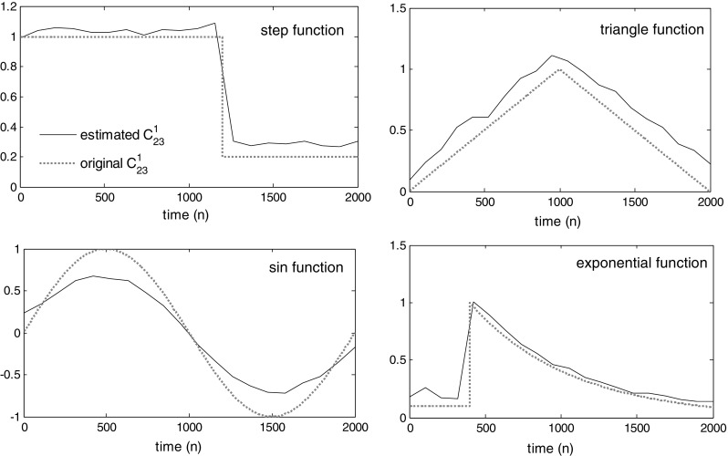
Different functions as coefficients. Estimated coefficient is plotted as solid line, and original signal is drawn by dashed line. The tv-CREANN can trace different types of time-varying signals
-
B.
Changing with various frequencies:
In addition to various shapes of time-varying , we also examine the network’s capability in following coefficient’s change at different frequencies. In other words we want to evaluate our method’s performance in the case of rapid/slow changes in interaction strengths over time. The simulation results for the various frequencies are shown in Fig. 10. This shows that our method can also track rapid changing coefficients. However, for following the rapid changes, tv-CREANN method is delayed because of limitations in choosing a relatively large data length.
Fig. 10.

Time-varying coefficients in different frequencies. Estimated coefficient is plotted as solid black line, and original signal is drawn by dashed gray line
Model validation
To validate the applied model, three validation factors were introduced in “Validation the model” section. If the neural network is well trained by the examples, it would produce a relatively small training error, and if it shows an acceptable generalization performance, the testing error would be in the range of training error (in this study we considered the first 90% of data in each segment as the training, and the last 10% as testing data). Finally if the MVAR model is well-fitted to the data, the residual is expected to behave like the white noise; i.e. the autocorrelation function of error signal should be similar to an impulse function (Cohen and Cauwenberghs 1998). Table 7 contains the training and testing error for the simulated model with time-varying coefficients. These results satisfy the two first factors for a validated model.
Table 7.
Training and testing error of ANN for various condition of simulation (left panel: various model orders, right panel: various SNRs). Testing error is in the range of training error
| Maximum time lag (model order) | SNR (dB) | ||||||||||
|---|---|---|---|---|---|---|---|---|---|---|---|
| p = 2 | p = 3 | p = 4 | p = 5 | p = 6 | p = 7 | 20 dB | 10 dB | 0 dB | 10 dB | 20 dB | |
| Training error | 0.182 | 0.18 | 0.181 | 0.179 | 0.176 | 0.177 | 0.177 | 0.029 | 0.02 | 0.011 | 0.007 |
| Testing error | 0.177 | 0.206 | 0.194 | 0.184 | 0.214 | 0.196 | 0.182 | 0.033 | 0.019 | 0.012 | 0.007 |
For the third factor, we compute the autocorrelation function of network error. This error is the difference between the network’s targets and the outputs. Figure 11 obviously shows the whiteness of the error (model residuals) and emphasizes on the validated model.
Fig. 11.

Autocorrelation function of ANN errors (error was computed for every data sample). The impulse autocorrelation function reveals that the error (model residual) behaves as white noise
Applying the method on EEG data
After evaluation the method with simulated data, the tv-CREANN algorithm is applied to EEG signals, recorded from healthy subjects that participated to a recognition memory task. The data is belonging to the database, previously published along with a standard ERP analysis by Curran et al. (2006). The stimuli were low-frequency English words. If the subject truly remembered the previously studied old word, the condition was named “Hit”, while the “CR” condition was defined when the subject correctly rejected the unstudied new words. As a case study, our method is applied on the data of three subjects. For these subjects, there were almost 100 trials for Hit and 100 trials for CR conditions. During the task, 128-channel scalp voltages were recorded from 100 ms before to 1000 ms after presenting the stimulus, with the sampling rate of 250 Hz. ERPs were obtained by stimulus-locked averaging of every 10 EEG recordings in each Hit/CR condition. The ERPs were baseline-corrected with respect to a 100 ms pre-stimulus recording interval, and were passed through a low-pass causal FIR filter with the cutoff frequency of 45 Hz (For more details, please refer to [59]).
Preprocessing prior to tv-CREANN analysis
EEG signals suffer from volume conduction effect, which may cause serious confounding results when effective connectivity assessed based on the these scalp voltages (Nunez and Srinivasan 2006). A plausible attempt in dealing with the volume conduction effect is to first apply inverse methods on EEG recordings, and then estimating the effective connectivity patterns (Schoffelen and Gross 2009; Supp et al. 2007). For source reconstruction procedure, in this study we use Statistical Parametric Mapping (SPM) software package in “standard” inversion setting, which applies multiple sparse priors (MSP) algorithm (Friston et al. 2008). The SPM toolbox is available online at http://www.fil.ion.ucl.ac.uk/spm/.
After estimating and localizing the underlying brain sources, the time courses of regions of interest (ROIs) with maximal activities, are considered for tv-CREANN analysis. These sources are common to both Hit/CR conditions. The MNI coordinates (defined by Montreal Neurological Institute) of the local maximum of the selected regions, their corresponding Brodmann areas (Brodmann 2006), and their neuroanatomical labels are summarized in Table 8. The occipital regions are active in response to the visual demands of the task. The motor cortex is also active; presumably because of the demand for the subjects to make a button press. Furthermore, activated regions are observed in the frontal, temporal and parietal areas. This activation pattern has been reported in previous episodic retrieval studies (Eichenbaum et al. 2007; Rugg et al. 1996; Rugg and Henson 2002; Vilberg and Rugg 2008).
Table 8.
Coordinates and labels of ROIs (regions with maximal activity considered for the analysis)
| Region number | MNI coordinates [X Y Z] | Brodman area | Neuroanatomical label |
|---|---|---|---|
| 1 | [26 62 −4] | R-BA10 | Prefrontal cortex |
| 2 | [−16 62 −6] | L-BA10 | Prefrontal cortex |
| 3 | [10 10 66] | R-BA6 | Motor area |
| 4 | [−6 10 68] | L-BA6 | Motor area |
| 5 | [56 −50 −20] | R-BA37 | Medial temporal |
| 6 | [−54 −51 −21] | L-BA37 | Medial temporal |
| 7 | [16 −56 68] | R-BA7 | Superior parietal |
| 8 | [−16 −54 68] | L-BA7 | Superior parietal |
| 9 | [22 −80 34] | R-BA19 | Inferior occipital |
| 10 | [−20 −82 34] | L-BA19 | Inferior occipital |
Implementation of tv-CREANN for memory retrieval data
Since the task-related interactions between the regions may vary through the time, the data length is divided into N = 5 segments of 220 ms, and the connectivity pattern is estimated for each segment. The considered model order (p opt = 7), is the minimum estimated order by evaluating the SBC over the entire data using the ARFIT toolbox (Schneider and Neumaier 2001), and also based on mutual information measure (refer to “Input selection (choice of model order)” section). Because of a large number of unknown parameters, for every time segment, we increased the length of data by putting the segments of all trials into a single vector; assuming that at that time interval the behavior of brain regions and their interactions are similarly represented in all trials. Furthermore, we set number of hidden neurons, N h = 5, as small as possible (as increasing the number of hidden neurons did not significantly improve the training and testing error).
The tv-CREANN is then applied on preprocessed data. For validation of the estimations, the autocorrelation function of network error is computed for all data segments of all ROIs. Figure 12 shows the whiteness of the error and emphasis on the validated model.
Fig. 12.
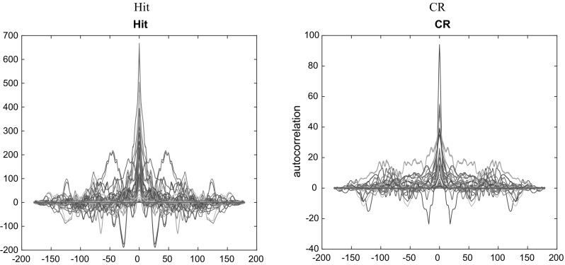
The impulse autocorrelation function of error for Hit (left) and CR (right), computed for all data segments of all ROIs, shows the whiteness of error
The estimated time-varying Causality coefficient (c dij) measures are presented on the typical head shape. The selected ROIs are shown by the numbers described in Table 8. The connectivity links are represented by arrows, pointing from one region toward another one (Fig. 13). The size of the arrows is corresponded to the connectivity strength (i.e. the c dij values). The histogram of all coefficients c dijs is plotted. The coefficients have a zero-mean normal distribution, and the threshold for the line thickness of the arrows is considered with respect to their distribution standard deviation (SD). Furthermore, the line style is determined by the sign of the coefficient. Positive c dijs are depicted by red solid arrows, while the negative c dijs are shown by blue dotted arrows.
Fig. 13.
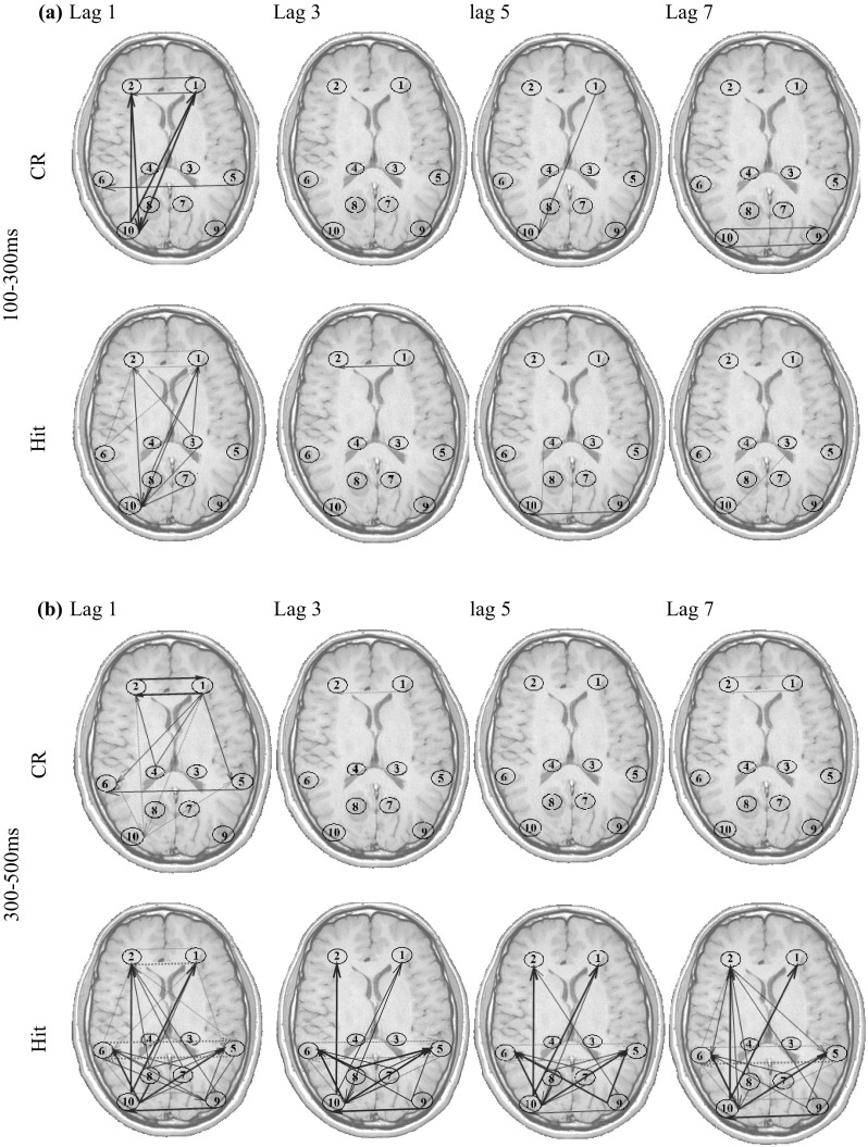
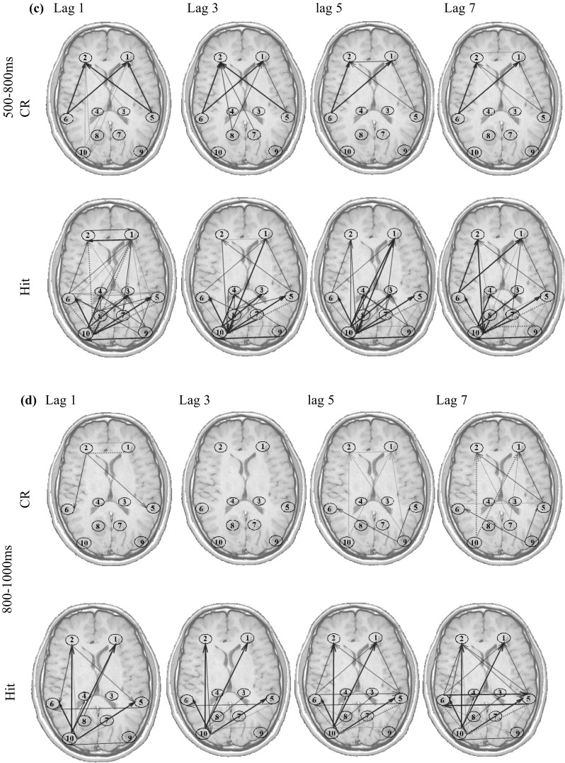
Time-varying effective connectivity patterns for Hit and CR conditions. The ROI numbers are identical to those in Table 8. Positive connectivity is shown by Red-solid and negative connectivity is shown by blue-dotted arrows with the thickness of the line corresponding to the strength of effective connectivity. If |c dij| < 2*SD, there is no connecting arrow between the regions. 2*SD < |c dij| < 4*SD correspond to thin arrows and |c dij| > 4*SD is shown by thick arrows. The SD is the standard deviation of all s distribution. (Color figure online)
The arrows in Fig. 13 show the effective connectivity patterns. For brevity, the influence of the regions’ past on the present activity is only shown for lags d = 1, 3, 5, 7 (i.e. ). Furthermore, because there is no significant effective connectivity in 100 before to 100 ms after presenting the stimulus, the connectivity patterns of this time interval is not displayed.
From these results, it is possible to note time-varying patterns of effective connectivity during the memory retrieval process. The tv-CREANN evaluation reveals prominent information flow between frontal (ROI #1, ROI #2) and (left) occipital (ROI #9) regions, started from 100 ms post-stimuli and maintained up to 1000 ms. Furthermore, the temporal (ROI #5, ROI # 6)-frontal (ROI #1, ROI #2), and temporal (ROI #5, ROI #6)– occipital (ROI #9, ROI #10) interaction is dominant after 300 ms post-stimuli onset.
The increased activity of these regions has been previously reported in many studies (e.g. see Cansino et al. 2002; Hampstead et al. 2011; Parker et al. 2005). These results are also in accordance with the connectivity studies in episodic memory (Lee and Zhang 2014; Watrous et al. 2013). The authors reported significant information flow increases between frontal cortex, and specific sub-regions of medial temporal, parietal and occipital regions when participants retrieved the episodic memory.
In addition to these connectivity patterns which are common in both Hit and CR, the results show some differences between these two conditions. The most prominent difference is the information flow between parietal (ROI #7, ROI #8) and other regions, which is more significant in Hit condition. The other difference between old and new item retrieval is seen in greater interaction between temporal (ROI #5, ROI #6) and occipital (ROI #9, ROI #10) regions in Hit. These results are discussed in the next section.
Discussion
Inspired by human brain system and regarding to the capabilities of artificial neural networks in system identification, the present study tries to estimate effective connectivity patterns by an ANN’s model information. In other words, because of being a universal approximator, training an MLP neural network, with inputs of lagged samples of the data, would predict the subsequent samples with reasonable accuracy and precision. This ANN behaves as a nonlinear multivariate autoregressive model. To extract the information embedded within this model, we defined the Causality coefficient measure with regard to the network’s structure and activation functions of its neurons. Causality coefficient has some advantages, compared with the previously defined measure of multiplying network weights. In addition to more accurate estimation of coefficients, in the repetition of the procedure, there are less variance of the results for Causality coefficient method than multiplying network weights. This demonstrates that considering all network parameters in Causality coefficient performs better than just using the connecting weights, and it does not have the problem of repeatability and consistency, reported for the measure of multiplying network weights (Gevrey et al. 2003).
To evaluate our proposed method, we performed series of simulations including the MVAR models. For time-varying analysis we divided data into (non-overlapping) windows, on the logic that shorter windows are more likely to be approximately stationary and can better show changes over time. However, the window length should be large enough to adequately train the network and properly fit the model to the data. Another important factor to have a reliable estimation of effective connectivity using classical MVAR models, is the choice of the correct model order. If the order is too high, the model overfits, and unwanted components overshadowing the correct ones and instabilities occur. Porcaro et al. (2009) showed that the use of an overestimated order is hazardous in real applications. By estimating PDC and DTF, they revealed that, in case of overestimated order, extra-connections appeared or very important connections were lacking in their connectivity network. Furthermore, if the order is too low, the model cannot capture the essential dynamics of the data. Gourevitch et al. (2006) showed that on the simulated data, an underestimate model order has also been critical for the connectivity correctness (Gourévitch et al. 2006). However, our simulation results indicate that the CREANN shows robustness with respect to the choice of the model order; if the intended delay for the past samples of signals is more than its actual value (i.e. Max-lag > p opt), the estimation error for the coefficients does not change significantly, and the coefficients c dji are estimated close to zero for d > p opt (c.f. Fig. 6).
The other big challenge in using EEGs is the very small signal-to-noise ratio of the brain signals. In fact, the cerebral signals related to significant physiological activity recorded on the scalp are mixed and embedded in unstructured noise and other physiological signals unrelated to the phenomena under investigation (Porcaro et al. 2009). If there is a method that can appropriately act in various noise levels, the computational cost and difficulties related to the noise reduction processes will be reduced. ANNs have the ability to tolerate noisy data, and frequently outperform traditional statistical methods (Biswas et al. 2016; Hang et al. 2009). Our results emphasize the capability of the CREANN method in dealing with noisy data at various SNRs (Fig. 8). This valuable advantage is particularly important for the analysis of brain signals.
Furthermore, the simulation results indicate that the method can estimate changes (various shapes of changing at the different frequency) in effective connectivity through the time. These significant features made it potentially an interesting, reasonable and useful tools for estimating effective connectivity.
After evaluating the performance of the tv-CREANN method by simulated models, it was applied on the real EEG signals recorded during a memory recognition task. An overall inspection of the results (Fig. 13) suggests that episodic memory retrieval could be characterized by increased information flows between the prefrontal cortex, medial temporal lobe, occipital and the parietal cortex.
The sustained interaction between the prefrontal cortex (within the frontal lobes) with occipital (and other) regions emphasizes on its crucial role in memory tasks. Most models proposed that the main storage site of information is not within the frontal lobes themselves, but in the posterior cortex, and that the prefrontal functioning is to keep this information active and/or manipulate the active information according to current goals (Ward 2015). Furthermore, the causal relationship between temporal and other regions may be due to the well-known critical role of medial temporal lobe (MTL) in conscious recognition memory (Danckert et al. 2007). There are various suggesting descriptions about the function of different structures in MTL and their interactions with other brain regions. The MTL may be involved in the permanent storage of certain kinds of memory in addition to supporting consolidation (Mayes 1988), or it may bind together different aspects of memory (e.g. perceptual, affective, linguistic components) represented in disparate regions of the brain (Frankland and Bontempi 2005) [for more details please refer to Ward (2015)]. It may acts as a hub for interactions between different regions during retrieving an episode (Watrous et al. 2013). Therefore, to retrieve the items’ information the MTL has a key interaction with others.
Besides similar effective connectivity network for Hits and CRs, which is probably generated by common basic retrieval processes, the results of this study showed some more interactions between parietal regions are and the others, and also between temporal and occipital regions, in the case of old item retrieval (Hits).
Many event-related potentials (ERP), as well as event-related fMRI studies, have documented differential parietal contributions to episodic retrieval for correctly recognize old items (Hit) as compared with correctly identifying new items (CR). This difference called ‘old/new’ effects (alternatively labeled ‘retrieval success’ effects) is associated with increased positivity between 500 and 800 ms post-stimulus onset in ERPs, and greater activation measured by fMRI imaging, during Hit than during CR in parietal cortex (Wagner et al. 2005; Weis et al. 2004). Increased effective connectivity in Hit condition rather than the CR may be explained by different theories (Kim 2013). The parietal region might contribute to shifting attention to, or maintain attention on, internally generated mnemonic representations. It may support the mental re-experiencing of an old event or ecphory (Tulving 1985), or more strategic retrieval processes, such as iterative searches and verification of retrieved information, which may engage more consistently during a Hit than during a CR (Buckner 2003).
Despite the well-established role of MTL in episodic memory, the old/new effects for this region is controversial (Kim 2013). Several studies proposed that retrieval-related MTL activity (old > new) occurs, while there are some reports of New/old (CR > hit) effects, most strongly associated with the bilateral medial temporal lobe, and possibly reflecting greater encoding-related activity for new than for old items (Danckert et al. 2007; Kim 2013). The increased interaction between the temporal and occipital region in our study may be explained by the reports of involving occipital region (BA 19) in processing the phonological properties of words (Dietz et al. 2005), with old activity greater than new activity (likely reflecting priming) (Slotnick and Schacter 2006).
However, we emphasize that these proposals are theoretical, and may provide preliminary knowledge about causal relationships in the brain during retrieving an episode. Applying the method on additional data, will be required to refine and test these ideas (which is our future work). Furthermore, there are some notable issues should be considered in the future works.
For the sake of simplicity, in this study we simulated linear MVAR models and examined our proposed method in estimating time-invariant and time-varying coefficients. Therefore, as some studies assumed that the interactions among neuronal populations are nonlinear (Khadem and Hossein-Zadeh 2014; Marinazzo et al. 2011; Pereda et al. 2005), using the nonlinear connectivity measures may outperform linear measures, and can give better insight into brain mechanisms. Extracting nonlinear causal relationships between brain regions is one of our desired future works. However, it has been concluded by several researchers that although nonlinear methods (Roulston 1999; Stam and Van Dijk 2002) might be preferred when studying EEG broadband signals, the linear measurements are still convenient since they afford a rapid and straightforward characterization of connectivity patterns (Astolfi et al. 2008).
In addition to nonlinearity schemes, it should be noted that an important factor in estimating effective connectivity for EEG and MEG signals is the “volume conduction effect” (He et al. 2011). Estimating effective connectivity from reconstructed sources is one possible approach to reduce this effect. However, extracting underlying sources from EEG signals is time-consuming and due to the ill-posed nature of the EEG/MEG inverse problem, a fully satisfactory inverse method may not exist (Sarvas 1987). For our future work, the volume conduction effect will also be taken into consideration in estimating effective connectivity by means of an artificial neural network.
Acknowledgements
We are thankful to Professor Tim Curran and his co-authors for providing the EEG data. This research is supported by Cognitive Sciences and technologies Council of Iran, under the Grant Number 2688.
References
- Addis DR, Moscovitch M, McAndrews MP. Consequences of hippocampal damage across the autobiographical memory network in left temporal lobe epilepsy. Brain. 2007;130(Pt 9):2327–2342. doi: 10.1093/brain/awm166. [DOI] [PubMed] [Google Scholar]
- Ashby FG, Ell SW, Valentin VV, Casale MB. FROST: a distributed neurocomputational model of working memory maintenance. J Cogn Neurosci. 2005;17(11):1728–1743. doi: 10.1162/089892905774589271. [DOI] [PubMed] [Google Scholar]
- Astolfi L, Cincotti F, Babiloni C, Carducci F, Basilisco A, Rossini PM, Babiloni F. Estimation of the cortical connectivity by high-resolution EEG and structural equation modeling: simulations and application to finger tapping data. IEEE Trans Biomed Eng. 2005;52(5):757–768. doi: 10.1109/TBME.2005.845371. [DOI] [PubMed] [Google Scholar]
- Astolfi L, Cincotti F, Mattia D, Marciani MG, Baccala LA, de Vico Fallani F, Babiloni F. Assessing cortical functional connectivity by partial directed coherence: simulations and application to real data. IEEE Trans Biomed Eng. 2006;53(9):1802–1812. doi: 10.1109/TBME.2006.873692. [DOI] [PubMed] [Google Scholar]
- Astolfi L, Cincotti F, Mattia D, Marciani MG, Baccala LA, de Vico Fallani F, Babiloni F. Comparison of different cortical connectivity estimators for high-resolution EEG recordings. Hum Brain Mapp. 2007;28(2):143–157. doi: 10.1002/hbm.20263. [DOI] [PMC free article] [PubMed] [Google Scholar]
- Astolfi L, Cincotti F, Mattia D, De Vico Fallani F, Tocci A, Colosimo A, Babiloni F. Tracking the time-varying cortical connectivity patterns by adaptive multivariate estimators. IEEE Trans Biomed Eng. 2008;55(3):902–913. doi: 10.1109/TBME.2007.905419. [DOI] [PubMed] [Google Scholar]
- Atmanspacher H, Rotter S. Interpreting neurodynamics: concepts and facts. Cogn Neurodyn. 2008;2(4):297–318. doi: 10.1007/s11571-008-9067-8. [DOI] [PMC free article] [PubMed] [Google Scholar]
- Baba K, Enbutu I, Yoda M (1990) Explicit representation of knowledge acquired from plant historical data using neural network. Paper presented at the 1990 IJCNN International Joint Conference on Neural Networks, 1990
- Baccala LA, Alvarenga MY, Sameshima K, Jorge CL, Castro LH. Graph theoretical characterization and tracking of the effective neural connectivity during episodes of mesial temporal epileptic seizure. J Integr Neurosci. 2004;3(4):379–395. doi: 10.1142/S0219635204000610. [DOI] [PubMed] [Google Scholar]
- Behnam H, Sheikhani A, Mohammadi MR, Noroozian M, Golabi P (2008) Abnormalities in connectivity of quantitative electroencephalogram background activity in autism disorders especially in left hemisphere and right temporal. Paper presented at the tenth international conference on computer modeling and simulation (uksim 2008)
- Biswas SK, Marbaniang L, Purkayastha B, Chakraborty M, Singh HR, Bordoloi M. Rainfall forecasting by relevant attributes using artificial neural networks-a comparative study. Int J Big Data Intell. 2016;3(2):111–121. doi: 10.1504/IJBDI.2016.077362. [DOI] [Google Scholar]
- Bitan T, Booth JR, Choy J, Burman DD, Gitelman DR, Mesulam MM. Shifts of effective connectivity within a language network during rhyming and spelling. J Neurosci. 2005;25(22):5397–5403. doi: 10.1523/JNEUROSCI.0864-05.2005. [DOI] [PMC free article] [PubMed] [Google Scholar]
- Boger Z, Guterman H (1997) Knowledge extraction from artificial neural network models. Paper presented at the 1997 IEEE international conference on systems, man, and cybernetics, 1997. Computational cybernetics and simulation
- Bowden GJ, Dandy GC, Maier HR. Input determination for neural network models in water resources applications. Part 1—background and methodology. J Hydrol. 2005;301(1):75–92. doi: 10.1016/j.jhydrol.2004.06.021. [DOI] [Google Scholar]
- Bressler SL, Richter CG, Chen Y, Ding M. Cortical functional network organization from autoregressive modeling of local field potential oscillations. Stat Med. 2007;26(21):3875–3885. doi: 10.1002/sim.2935. [DOI] [PubMed] [Google Scholar]
- Brodmann K (2006) Brodmann’s: localisation in the cerebral cortex (Garey LJ, trans.). Springer US
- Broman KW, Speed TP. A model selection approach for the identification of quantitative trait loci in experimental crosses. J R Stat Soc Ser B (Stat Methodol) 2002;64(4):641–656. doi: 10.1111/1467-9868.00354. [DOI] [Google Scholar]
- Brunet D, Murray MM, Michel CM. Spatiotemporal analysis of multichannel EEG: CARTOOL. Comput Intell Neurosci. 2011;2011:813870. doi: 10.1155/2011/813870. [DOI] [PMC free article] [PubMed] [Google Scholar]
- Buckner RL. Functional–anatomic correlates of control processes in memory. J Neurosci. 2003;23(10):3999–4004. doi: 10.1523/JNEUROSCI.23-10-03999.2003. [DOI] [PMC free article] [PubMed] [Google Scholar]
- Burge J, Lane T, Link H, Qiu S, Clark VP. Discrete dynamic Bayesian network analysis of fMRI data. Hum Brain Mapp. 2009;30(1):122–137. doi: 10.1002/hbm.20490. [DOI] [PMC free article] [PubMed] [Google Scholar]
- Cadotte AJ, Mareci TH, DeMarse TB, Parekh MB, Rajagovindan R, Ditto WL, Carney PR. Temporal lobe epilepsy: anatomical and effective connectivity. IEEE Trans Neural Syst Rehabil Eng. 2009;17(3):214–223. doi: 10.1109/TNSRE.2008.2006220. [DOI] [PubMed] [Google Scholar]
- Cansino S, Maquet P, Dolan RJ, Rugg MD. Brain activity underlying encoding and retrieval of source memory. Cereb Cortex. 2002;12(10):1048–1056. doi: 10.1093/cercor/12.10.1048. [DOI] [PubMed] [Google Scholar]
- Cheung BL, Nowak R, Lee HC, van Drongelen W, Van Veen BD. Cross validation for selection of cortical interaction models from scalp EEG or MEG. IEEE Trans Biomed Eng. 2012;59(2):504–514. doi: 10.1109/TBME.2011.2174991. [DOI] [PMC free article] [PubMed] [Google Scholar]
- Chuang CH, Huang CS, Lin CT, Ko LW, Chang JY, Yang JM (2012, 4-6 June 2012) Mapping information flow of independent source to predict conscious level: a granger causality based brain–computer interface. Paper presented at the 2012 international symposium on computer, consumer and control
- Coben R, Chabot RJ, Hirshberg L. EEG analyses in the assessment of autistic disorders. In: Casanova MF, El-Baz AS, Suri JS, editors. In: Imaging the brain in autism. New York: Springer; 2013. pp. 349–370. [Google Scholar]
- Coben R, Mohammad-Rezazadeh I, Cannon RL (2014) Using quantitative and analytic EEG methods in the understanding of connectivity in autism spectrum disorders: a theory of mixed over- and under-connectivity. Front Hum Neurosci 8(45). doi:10.3389/fnhum.2014.00045 [DOI] [PMC free article] [PubMed]
- Cohen M, Cauwenberghs G (1998) Blind separation of linear convolutive mixtures through parallel stochastic optimization. Paper presented at the proceedings of the 1998 IEEE international symposium on circuits and systems, 1998. ISCAS’98
- Curran T, DeBuse C, Woroch B, Hirshman E. Combined pharmacological and electrophysiological dissociation of familiarity and recollection. J Neurosci. 2006;26(7):1979–1985. doi: 10.1523/JNEUROSCI.5370-05.2006. [DOI] [PMC free article] [PubMed] [Google Scholar]
- Danckert S, Gati J, Menon R, Köhler S. Perirhinal and hippocampal contributions to visual recognition memory can be distinguished from those of occipito-temporal structures based on conscious awareness of prior occurrence. Hippocampus. 2007;17(11):1081–1092. doi: 10.1002/hipo.20347. [DOI] [PubMed] [Google Scholar]
- Dietz NA, Jones KM, Gareau L, Zeffiro TA, Eden GF. Phonological decoding involves left posterior fusiform gyrus. Hum Brain Mapp. 2005;26(2):81–93. doi: 10.1002/hbm.20122. [DOI] [PMC free article] [PubMed] [Google Scholar]
- Eichenbaum H, Yonelinas AP, Ranganath C. The medial temporal lobe and recognition memory. Annu Rev Neurosci. 2007;30:123–152. doi: 10.1146/annurev.neuro.30.051606.094328. [DOI] [PMC free article] [PubMed] [Google Scholar]
- Faes L, Nollo G. Extended causal modeling to assess Partial Directed Coherence in multiple time series with significant instantaneous interactions. Biol Cybern. 2010;103(5):387–400. doi: 10.1007/s00422-010-0406-6. [DOI] [PubMed] [Google Scholar]
- Frankland PW, Bontempi B. The organization of recent and remote memories. Nat Rev Neurosci. 2005;6(2):119–130. doi: 10.1038/nrn1607. [DOI] [PubMed] [Google Scholar]
- Friston K. Functional and effective connectivity in neuroimaging: a synthesis. Hum Brain Mapp. 1994;2(1–2):56–78. doi: 10.1002/hbm.460020107. [DOI] [Google Scholar]
- Friston KJ, Harrison L, Penny W. Dynamic causal modelling. Neuroimage. 2003;19(4):1273–1302. doi: 10.1016/S1053-8119(03)00202-7. [DOI] [PubMed] [Google Scholar]
- Friston K, Harrison L, Daunizeau J, Kiebel S, Phillips C, Trujillo-Barreto N, Mattout J. Multiple sparse priors for the M/EEG inverse problem. Neuroimage. 2008;39(3):1104–1120. doi: 10.1016/j.neuroimage.2007.09.048. [DOI] [PubMed] [Google Scholar]
- Gevrey M, Dimopoulos I, Lek S. Review and comparison of methods to study the contribution of variables in artificial neural network models. Ecol Model. 2003;160(3):249–264. doi: 10.1016/S0304-3800(02)00257-0. [DOI] [Google Scholar]
- Ghasemi M, Mahloojifar A (2012, 20–21 Dec. 2012) Directed transform function approach for functional network analysis in resting state fMRI data of Parkinson disease. Paper presented at the 2012 19th Iranian conference of biomedical engineering (ICBME)
- Giannakakis GA, Nikita KS (2008) Estimation of time-varying causal connectivity on EEG signals with the use of adaptive autoregressive parameters. Paper presented at the Engineering in Medicine and Biology Society, 2008. EMBS 2008. 30th annual international conference of the IEEE [DOI] [PubMed]
- Gourévitch B, Le Bouquin-Jeannès R, Faucon G. Linear and nonlinear causality between signals: methods, examples and neurophysiological applications. Biol Cybern. 2006;95(4):349–369. doi: 10.1007/s00422-006-0098-0. [DOI] [PubMed] [Google Scholar]
- Gravier A, Quek C, Duch W, Wahab A, Gravier-Rymaszewska J. Neural network modelling of the influence of channelopathies on reflex visual attention. Cogn Neurodyn. 2016;10(1):49–72. doi: 10.1007/s11571-015-9365-x. [DOI] [PMC free article] [PubMed] [Google Scholar]
- Hampstead BM, Stringer AY, Stilla RF, Deshpande G, Hu X, Moore AB, Sathian K. Activation and effective connectivity changes following explicit-memory training for face-name pairs in patients with mild cognitive impairment: a pilot study. Neurorehabil Neural Repair. 2011;25(3):210–222. doi: 10.1177/1545968310382424. [DOI] [PMC free article] [PubMed] [Google Scholar]
- Hang X, HaoT, Yu-He L (2009, 12–15 July 2009) Time series prediction based on NARX neural networks: an advanced approach. Paper presented at the 2009 international conference on machine learning and cybernetics
- Hannart A, Naveau P. An improved Bayesian information criterion for multiple change-point models. Technometrics. 2012;54(3):256–268. doi: 10.1080/00401706.2012.694780. [DOI] [Google Scholar]
- He B, Yang L, Wilke C, Yuan H. Electrophysiological imaging of brain activity and connectivity-challenges and opportunities. IEEE Trans Biomed Eng. 2011;58(7):1918–1931. doi: 10.1109/TBME.2011.2139210. [DOI] [PMC free article] [PubMed] [Google Scholar]
- Hemmelmann D, Ungureanu M, Hesse W, Wüstenberg T, Reichenbach J, Witte O, Leistritz L. Modelling and analysis of time-variant directed interrelations between brain regions based on BOLD-signals. Neuroimage. 2009;45(3):722–737. doi: 10.1016/j.neuroimage.2008.12.065. [DOI] [PubMed] [Google Scholar]
- Hesse W, Möller E, Arnold M, Schack B. The use of time-variant EEG Granger causality for inspecting directed interdependencies of neural assemblies. J Neurosci Methods. 2003;124(1):27–44. doi: 10.1016/S0165-0270(02)00366-7. [DOI] [PubMed] [Google Scholar]
- Hill DC, McMillan D, Bell KR, Infield D. Application of auto-regressive models to UK wind speed data for power system impact studies. IEEE Trans Sustain Energy. 2012;1:134–141. doi: 10.1109/TSTE.2011.2163324. [DOI] [Google Scholar]
- Horwitz B. The elusive concept of brain connectivity. Neuroimage. 2003;19(2 Pt 1):466–470. doi: 10.1016/S1053-8119(03)00112-5. [DOI] [PubMed] [Google Scholar]
- Hytti H, Takalo R, Ihalainen H. Tutorial on multivariate autoregressive modelling. J Clin Monit Comput. 2006;20(2):101–108. doi: 10.1007/s10877-006-9013-4. [DOI] [PubMed] [Google Scholar]
- Khadem A, Hossein-Zadeh GA. Estimation of direct nonlinear effective connectivity using information theory and multilayer perceptron. J Neurosci Methods. 2014;229:53–67. doi: 10.1016/j.jneumeth.2014.04.008. [DOI] [PubMed] [Google Scholar]
- Kim H. Differential neural activity in the recognition of old versus new events: an activation likelihood estimation meta-analysis. Hum Brain Mapp. 2013;34(4):814–836. doi: 10.1002/hbm.21474. [DOI] [PMC free article] [PubMed] [Google Scholar]
- Kundu B, Sutterer DW, Emrich SM, Postle BR. Strengthened effective connectivity underlies transfer of working memory training to tests of short-term memory and attention. J Neurosci. 2013;33(20):8705–8715. doi: 10.1523/JNEUROSCI.5565-12.2013. [DOI] [PMC free article] [PubMed] [Google Scholar]
- Lee CY, Zhang BT (2014) Effective EEG connectivity analysis of episodic memory retrieval. Paper presented at the proceedings of annual meeting of the Cognitive Science Society (CogSci 2014)
- Lehnertz K. Assessing directed interactions from neurophysiological signals—an overview. Physiol Meas. 2011;32(11):1715–1724. doi: 10.1088/0967-3334/32/11/R01. [DOI] [PubMed] [Google Scholar]
- Liu Z, Zhang Y, Bai L, Yan H, Dai R, Zhong C, Feng Y. Investigation of the effective connectivity of resting state networks in Alzheimer’s disease: a functional MRI study combining independent components analysis and multivariate Granger causality analysis. NMR Biomed. 2012;25(12):1311–1320. doi: 10.1002/nbm.2803. [DOI] [PubMed] [Google Scholar]
- Marinazzo D, Liao W, Chen H, Stramaglia S. Nonlinear connectivity by Granger causality. Neuroimage. 2011;58(2):330–338. doi: 10.1016/j.neuroimage.2010.01.099. [DOI] [PubMed] [Google Scholar]
- May RJ, Maier HR, Dandy GC, Fernando TMKG. Non-linear variable selection for artificial neural networks using partial mutual information. Environ Model Softw. 2008;23(10):1312–1326. doi: 10.1016/j.envsoft.2008.03.007. [DOI] [Google Scholar]
- Mayes AR. Human organic memory disorders. Cambridge: Cambridge University Press; 1988. [Google Scholar]
- McIntosh AR. Mapping cognition to the brain through neural interactions. Memory. 1999;7(5–6):523–548. doi: 10.1080/096582199387733. [DOI] [PubMed] [Google Scholar]
- McNorgan C, Joanisse MF. A connectionist approach to mapping the human connectome permits simulations of neural activity within an artificial brain. Brain Connect. 2014;4(1):40–52. doi: 10.1089/brain.2013.0174. [DOI] [PubMed] [Google Scholar]
- Neumaier A, Schneider T. Estimation of parameters and eigenmodes of multivariate autoregressive models. ACM Trans Math Softw: (TOMS) 2001;27(1):27–57. doi: 10.1145/382043.382304. [DOI] [Google Scholar]
- Nunez PL, Srinivasan R. Electric fields of the brain: the neurophysics of EEG. Oxford: Oxford University Press; 2006. [Google Scholar]
- Omidvarnia A, Azemi G, Boashash B, O’Toole JM, Colditz PB, Vanhatalo S. Measuring time-varying information flow in scalp EEG signals: orthogonalized partial directed coherence. IEEE Trans Biomed Eng. 2014;61(3):680–693. doi: 10.1109/TBME.2013.2286394. [DOI] [PubMed] [Google Scholar]
- Parker A, Bussey TJ, Wilding EL. The cognitive neuroscience of memory: encoding and retrieval. London: Psychology Press; 2005. [Google Scholar]
- Pereda E, Quiroga RQ, Bhattacharya J. Nonlinear multivariate analysis of neurophysiological signals. Prog Neurobiol. 2005;77(1–2):1–37. doi: 10.1016/j.pneurobio.2005.10.003. [DOI] [PubMed] [Google Scholar]
- Porcaro C, Zappasodi F, Rossini PM, Tecchio F. Choice of multivariate autoregressive model order affecting real network functional connectivity estimate. Clin Neurophysiol. 2009;120(2):436–448. doi: 10.1016/j.clinph.2008.11.011. [DOI] [PubMed] [Google Scholar]
- Protopapa F, Siettos CI, Myatchin I, Lagae L. Children with well controlled epilepsy possess different spatio-temporal patterns of causal network connectivity during a visual working memory task. Cogn Neurodyn. 2016;10(2):99–111. doi: 10.1007/s11571-015-9373-x. [DOI] [PMC free article] [PubMed] [Google Scholar]
- Rajapakse JC, Zhou J. Learning effective brain connectivity with dynamic Bayesian networks. Neuroimage. 2007;37(3):749–760. doi: 10.1016/j.neuroimage.2007.06.003. [DOI] [PubMed] [Google Scholar]
- Roulston MS. Estimating the errors on measured entropy and mutual information. Physica D. 1999;125(3):285–294. doi: 10.1016/S0167-2789(98)00269-3. [DOI] [Google Scholar]
- Rugg MD, Henson RN (2002) Episodic memory retrieval: an (event-related) functional neuroimaging perspective. In: The cognitive neuroscience of memory encoding and retrieval, pp 3–37
- Rugg MD, Fletcher PC, Frith CD, Frackowiak RS, Dolan RJ. Differential activation of the prefrontal cortex in successful and unsuccessful memory retrieval. Brain. 1996;119(Pt 6):2073–2083. doi: 10.1093/brain/119.6.2073. [DOI] [PubMed] [Google Scholar]
- Saad EW, Wunsch DC., II Neural network explanation using inversion. Neural Netw. 2007;20(1):78–93. doi: 10.1016/j.neunet.2006.07.005. [DOI] [PubMed] [Google Scholar]
- Sarvas J. Basic mathematical and electromagnetic concepts of the biomagnetic inverse problem. Phys Med Biol. 1987;32(1):11–22. doi: 10.1088/0031-9155/32/1/004. [DOI] [PubMed] [Google Scholar]
- Schneider T, Neumaier A. Algorithm 808: ARfit—a Matlab package for the estimation of parameters and eigenmodes of multivariate autoregressive models. ACM Trans Math Softw: (TOMS) 2001;27(1):58–65. doi: 10.1145/382043.382316. [DOI] [Google Scholar]
- Schoffelen JM, Gross J. Source connectivity analysis with MEG and EEG. Hum Brain Mapp. 2009;30(6):1857–1865. doi: 10.1002/hbm.20745. [DOI] [PMC free article] [PubMed] [Google Scholar]
- Sharma A. Seasonal to interannual rainfall probabilistic forecasts for improved water supply management: part 1—a strategy for system predictor identification. J Hydrol. 2000;239(1):232–239. doi: 10.1016/S0022-1694(00)00346-2. [DOI] [Google Scholar]
- Shibata R. Approximate efficiency of a selection procedure for the number of regression variables. Biometrika. 1984;71(1):43–49. doi: 10.1093/biomet/71.1.43. [DOI] [Google Scholar]
- Slotnick SD, Schacter DL. The nature of memory related activity in early visual areas. Neuropsychologia. 2006;44(14):2874–2886. doi: 10.1016/j.neuropsychologia.2006.06.021. [DOI] [PubMed] [Google Scholar]
- Sommerlade L, Henschel K, Wohlmuth J, Jachan M, Amtage F, Hellwig B, Schelter B. Time-variant estimation of directed influences during Parkinsonian tremor. J Physiol Paris. 2009;103(6):348–352. doi: 10.1016/j.jphysparis.2009.07.005. [DOI] [PubMed] [Google Scholar]
- Stam CJ, Reijneveld JC. Graph theoretical analysis of complex networks in the brain. Nonlinear Biomed Phys. 2007;1(1):3. doi: 10.1186/1753-4631-1-3. [DOI] [PMC free article] [PubMed] [Google Scholar]
- Stam C, Van Dijk B. Synchronization likelihood: an unbiased measure of generalized synchronization in multivariate data sets. Physica D. 2002;163(3):236–251. doi: 10.1016/S0167-2789(01)00386-4. [DOI] [Google Scholar]
- Stoica P, Selen Y. Model-order selection: a review of information criterion rules. IEEE Signal Process Mag. 2004;21(4):36–47. doi: 10.1109/MSP.2004.1311138. [DOI] [Google Scholar]
- Supp GG, Schlogl A, Trujillo-Barreto N, Muller MM, Gruber T. Directed cortical information flow during human object recognition: analyzing induced EEG gamma-band responses in brain’s source space. PLoS ONE. 2007;2(8):e684. doi: 10.1371/journal.pone.0000684. [DOI] [PMC free article] [PubMed] [Google Scholar]
- Tulving E. Elements of episodic memory. Oxford: Oup; 1985. [Google Scholar]
- Tuncer O, Shanker B, Kempel L. Tetrahedral-based vector generalized finite element method and its applications. IEEE Antennas Wirel Propag Lett. 2012;11:945–948. doi: 10.1109/LAWP.2012.2213291. [DOI] [Google Scholar]
- Valdes-Sosa PA, Roebroeck A, Daunizeau J, Friston K. Effective connectivity: influence, causality and biophysical modeling. Neuroimage. 2011;58(2):339–361. doi: 10.1016/j.neuroimage.2011.03.058. [DOI] [PMC free article] [PubMed] [Google Scholar]
- van der Velde F, de Kamps M. The necessity of connection structures in neural models of variable binding. Cogn Neurodyn. 2015;9(4):359–370. doi: 10.1007/s11571-015-9331-7. [DOI] [PMC free article] [PubMed] [Google Scholar]
- Vilberg KL, Rugg MD. Memory retrieval and the parietal cortex: a review of evidence from a dual-process perspective. Neuropsychologia. 2008;46(7):1787–1799. doi: 10.1016/j.neuropsychologia.2008.01.004. [DOI] [PMC free article] [PubMed] [Google Scholar]
- Wagner AD, Shannon BJ, Kahn I, Buckner RL. Parietal lobe contributions to episodic memory retrieval. Trends Cogn Sci. 2005;9(9):445–453. doi: 10.1016/j.tics.2005.07.001. [DOI] [PubMed] [Google Scholar]
- Wang R, Zhu Y. Can the activities of the large scale cortical network be expressed by neural energy? A brief review. Cogn Neurodyn. 2016;10(1):1–5. doi: 10.1007/s11571-015-9354-0. [DOI] [PMC free article] [PubMed] [Google Scholar]
- Ward J. The student’s guide to cognitive neuroscience. London: Psychology Press; 2015. [Google Scholar]
- Watrous AJ, Tandon N, Conner CR, Pieters T, Ekstrom AD. Frequency-specific network connectivity increases underlie accurate spatiotemporal memory retrieval. Nat Neurosci. 2013;16(3):349–356. doi: 10.1038/nn.3315. [DOI] [PMC free article] [PubMed] [Google Scholar]
- Weis S, Klaver P, Reul J, Elger CE, Fernández G. Temporal and cerebellar brain regions that support both declarative memory formation and retrieval. Cereb Cortex. 2004;14(3):256–267. doi: 10.1093/cercor/bhg125. [DOI] [PubMed] [Google Scholar]
- Wennekers T, Ay N. Finite state automata resulting from temporal information maximization and a temporal learning rule. Neural Comput. 2005;17(10):2258–2290. doi: 10.1162/0899766054615671. [DOI] [PubMed] [Google Scholar]
- Winterhalder M, Schelter B, Hesse W, Schwab K, Leistritz L, Klan D, Witte H. Comparison of linear signal processing techniques to infer directed interactions in multivariate neural systems. Signal Process. 2005;85(11):2137–2160. doi: 10.1016/j.sigpro.2005.07.011. [DOI] [Google Scholar]
- Wu X, Li J, Yao L (2012) Determining effective connectivity from FMRI data using a gaussian dynamic bayesian network. Paper presented at the neural information processing
- Zeng LL, Liao Y, Zhou Z, Shen H, Liu Y, Liu X, Hu D. Default network connectivity decodes brain states with simulated microgravity. Cogn Neurodyn. 2016;10(2):113–120. doi: 10.1007/s11571-015-9359-8. [DOI] [PMC free article] [PubMed] [Google Scholar]
- Zhang NR, Siegmund DO. A modified Bayes information criterion with applications to the analysis of comparative genomic hybridization data. Biometrics. 2007;63(1):22–32. doi: 10.1111/j.1541-0420.2006.00662.x. [DOI] [PubMed] [Google Scholar]